A hybrid one-then-two stage
algorithm for computationally
expensive electromagnetic design
optimization
Glenn Hawe
Vector Fields Ltd, Oxford, UK, and
Jan Sykulski
School of Electronics and Computer Science, University of Southampton,
Southampton, UK
Abstract
Purpose– The purpose of this paper is to propose a surrogate model-assisted optimization algorithm which effectively searches for the optimum at the earliest opportunity, avoiding the need for a large initial experimental design, which may be wasteful.
Design/methodology/approach– The methodologies of two-stage and one-stage selection of points are combined for the first time. After creating a small experimental design, a one-stage Kriging algorithm is used to search for the optimum for a fixed number of iterations. If it fails to locate the optimum, the points it samples are then used in lieu of a traditional experimental design to initialize a two-stage algorithm.
Findings– The proposed approach was tested on a mathematical test function. It was found that the optimum could be located, without necessarily constructing an accurate surrogate model first. The algorithm performed well on an electromagnetic design problem, outperforming both a random search and a genetic algorithm, in significantly fewer iterations. The results suggest a new interpretation of surrogate models – merely as tools for constructing a utility function to locate the optimum of an unknown function, as opposed to actual approximations of the unknown function.
Research limitations/implications– The research was carried out on unconstrained problems only. The findings have implications for modern experimental designs, as the proposed algorithm can often locate the optimum without necessarily constructing an accurate surrogate model.
Originality/value– The two paradigms of one-stage and two-stage selection of points in surrogate-model assisted optimization are combined for the first time. Also, it is believed that this is the first time that the methodology of one-stage optimization has been used in optimal electromagnetic design.
KeywordOptimization techniques Paper typeResearch paper
1. Introduction
In Jones (2001), surrogate-model assisted optimization algorithms are categorized into “two-stage” and “one-stage” varieties. At each iteration of a two-stage algorithm, a surrogate model is constructed from the observed data (the first stage), and then this model is used to determine where to sample next (the second stage) (Joneset al., 1998). Several different so-called utility functions (also referred to as infill sampling criteria) exist which are used to choose where to sample in the second stage, based on the surrogate model constructed in the first stage, (Jones, 2001; Jones et al., 1998;
The current issue and full text archive of this journal is available at
www.emeraldinsight.com/0332-1649.htm
COMPEL
26,2
236
COMPEL: The International Journal for Computation and Mathematics in Electrical and Electronic Engineering Vol. 26 No. 2, 2007
pp. 236-246
qEmerald Group Publishing Limited 0332-1649
Sasenaet al., 2002). The points which are sampled are then used in the reconstruction of the surrogate model during the first stage of the next iteration.
One-stage algorithms do not determine where to evaluate next based only on the observed data. In particular, they do not fit surrogate models to the observed data only. Instead, at each iteration, they choose where to sample next by determining the credibility of hypotheses made about the location of the global minimum. This is done by specifying a measure of credibility for a surrogate model (which may be viewed intuitively as being related to its smoothness, with smoother models being deemed more plausible), and then determining the credibility of surrogate models which pass through the observed data and each of the hypothesized optima (Gutmann, 2001). The point chosen to be sampled is the hypothesized optimum which has the most credible surrogate model passing through it.
The two-stage and one-stage approaches each have their own individual drawbacks. Two-stage approaches suffer from the fact that the surrogate model constructed in the first stage of an iteration may not be very accurate, resulting in a poor choice of point in the second stage. In particular, convergence to a false optimum (an optimum of the surrogate model, but not of the true function) can happen if uncertainty considerations are not made. Related to this is the issue of when to actually begin searching for the optimum. Before the iterations of the algorithm begin proper, an initial surrogate model is built using an experimental design, which is usually constructed to be space-filling in design variable space. However, it is not obvious how large this initial experimental design should be: if too few points are used, then the initial surrogate model may not be very accurate; conversely, if too many points are used, then evaluations will be wasted (Hawe and Sykulski, 2007).
One-stage methods suffer in that determining the credibility of a hypothesis is itself computationally expensive. For each hypothesis, a surrogate model must be constructed through the observed points and hypothesized point, in such a way that a measure of its credibility is maximized. This itself is an optimization problem, which increases in computational cost as the number of sampled points increases.
In this paper, a hybrid one-then-two stage surrogate model-assisted algorithm is proposed, which aims to overcome the shortcomings of each type of algorithm. In particular:
. the number of points chosen to be space-filling in design variable space (with
disregard to their objective function values) is very small in size (thereby reducing the risk of wasteful evaluations);
. the one-stage algorithm is not used when the number of examples sampled
exceeds a certain threshold (thereby keeping computational effort low); and
. the two stage optimization algorithm is not used with a surrogate model based
on a small number of points (i.e. the surrogate model used during the two-stage selection of points should be of a reasonable accuracy).
The method used to construct the surrogate model is Kriging, which is growing in popularity in the optimization of electromagnetic devices (Lebensztajnet al., 2004). For full details on Kriging, the reader is referred to Santneret al.(2003), or to Jones (2001) for a gentler introduction.
Electromagnetic
design
optimization
2. One-then-two stage algorithm
The proposed algorithm for locating the global minimum in d-dimensional design variable space D,Rd consists of three steps: initialization, one-stage selection of points, and two-stage optimization search.
2.1 Step 1: initialization
The only purpose of the initialization step is to sample enough points to allow a non-trivial Kriging model to be constructed (i.e. a model which is not a hyper-plane in
Rd). The space-filling Hammersley Sequence experimental design (Kalagnanam and Diwekar, 1997) of size 4d, is used to select the points. The experimental design size of 4dis significantly smaller than is normally used (10dis suggested in (Joneset al., 1998), for example), as the philosophy of this algorithm is to use information about objective function space to search for the minimum at the earliest possible opportunity. It should be noted, however, that as with the figure of 10d, the choice of 4d is guided by experience, rather than being based on theory.
2.2 Step 2: one-stage selection of points
Information about objective function space has now been obtained through sampling 4d points, and the aim in this second step is to use this information to strategically choose where to sample next. This is done using a one-stage Kriging algorithm. The use of a two-stage method at such an early stage would have been naive: any model fit to such a small number of points would likely have been inaccurate. However, using a one-stage method the selection of where to sample is not based on a model fit only to the observed points. Instead, given a hypothesis of the objective function value at the minimum, it samples the design vector which, if it took that objective function value, would yield the most credible Kriging model, given the points already sampled.
Making a single hypothesis consists of two parts: hypothesizing the objective function valuef*at the minimum, and hypothesizing the design vectorx*which takes
this objective function value. Whilst it is certainly the case that x*is unknown for
unsolved optimization problems, it may be the case thatf*is known. For example, in
many electromagnetic design problems, some objective functions may have ideal values (100 percent efficiency, for example), and these may be used as target values of
f*. If, however, no information is available for f* then its value may be estimated based on the observed points. For example, let the minimum objective function value of the points sampled so far be fmin, and let the maximum be fmax. f* may then be
constructed using f*¼fmin2q(fmax2fmin),fmin, where 0 , q. The value of q
may be varied at each iteration, using, for example:
q¼2ðimax2iÞ
imax
ð1Þ
whereiis the iteration number andimaxis the maximum number of iterations that will
be performed in this step. This has the effect of the search being quite exploratory to begin with, and gradually becoming more exploitative as the iterations proceed (as one would want).
Given a suitablef*the task of the one-stage algorithm is to determine thex*which,
if it had an objective function value of f* would yield the most credible response
surface. For Kriging models, the likelihood ofn sampled points, conditional upon a Kriging surface passing through (x*,f*) is (Jones, 2001):
COMPEL
26,2
1
ð2pÞn2ðs2Þj jC 1 2
exp 2ðy2mÞ
TC21ðy2mÞ
2s2
ð2Þ
where:
m¼1mþrðf*2mÞ ð3Þ
C¼R2rrT ð4Þ
are the conditional mean and correlation matrices. Here,R is then£n correlation matrix, whosei-j-th entry is:
Rðxi;xjÞ ¼Y
d
k¼1
exp 2ukxik2x j k
pk
ð5Þ
whereuk.0 andpk[½1;2.yis a vector of thenobjective function values,mis the
mean ands2 is the variance predicted by the Kriging model. The next point to be evaluated is the x* which maximizes (equation (2)). Note, that for each x*, the
credibility itself is maximized over the Kriging parametersm s,u¼[u1,u2,. . .,ud] and
p¼[p1,p2,. . .,pd]. In practice, however, it is the conditional log-likelihood:
2n
2 logðs
2Þ21
2logðj jÞC 2
ðy2mÞTC21ðy2mÞ
2s2 ð6Þ
which is maximized; furthermore, by setting the derivatives of equation (2) with respect tomandsto zero, yields:
s2¼ðy2mÞ
TC21ðy2mÞ
n ð7Þ
m¼1
TC21yþf
*rTC21r2yC21r2f
*1TC21r
1TC211221TC21rþrTC21r ð8Þ
meaning that equation (6) only needs to be optimized overu and p. Owing to the typical profile of log-likelihood plots, the Nelder and Mead (1965) simplex algorithm is used to maximize equation (6) for eachx*.
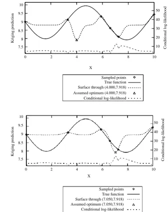
An illustration of this method of selecting points to evaluate is shown in Figure 1. The true function is given by Sasena (2002):
fðxÞ ¼2sinðxÞ2ex=100þ10 ð9Þ
and the global minimum, which has objective function valuef¼7.9182, is located at
x¼7.8648. The most credible Kriging surfaces for the following two hypotheses are shown:
H1. x*¼4.000 has objective function valuef*¼7.9182. H2. x*¼7.050 has objective function valuef*¼7.9182.
Electromagnetic
design
optimization
TheH1yields a surface with credibility (conditional log-likelihood) 4.772, whilst the
H2yields a surface with credibility 12.775. This agrees with our intuition about what a reasonable function should look like: the function in Figure 1(b) looks more plausible than the function in Figure 1(a).
[image:5.519.112.448.80.504.2]This step continues until the computational cost reaches a certain threshold. Given that a two-stage method is to be used in the next step, an appropriate point for terminating this stage is after 10devaluations have been made in total. It may be that the optimum is actually located within this number of evaluations (as is the case for
Figure 1.
(a) Kriging prediction for the hypothesis that the minimum of equation (9) is at (4.000, 7.918); (b) Kriging prediction for the hypothesis that the minimum of equation (9) is at (7.050, 7.918)
10
9.5
9
8.5
8
0 2 4 6
Sampled points
Conditional log-likelihood Assumed optimum (4.000,7.918) Surface through (4.000,7.918) True function X
8 10
50
Conditional log-likelihood
Kriging prediction
40
30
20
10 7.5
10
9.5
9
8.5
8
0 2 4 6
Sampled points
Conditional log-likelihood Assumed optimum (7.050,7.918) Surface through (7.050,7.918) True function X
8 10
50
Conditional log-likelihood
Kriging prediction
40
30
20
10 7.5
COMPEL
26,2
the test function reported in section 3); however, if it is not, the algorithm proceeds to step 3.
2.3 Step 3: two-stage optimization search
Proceeding to step 3 of the algorithm suggests one of two scenarios has arisen. Either: (1) the true optimal objective functionf*is known, but was not attained in step 2;
or
(2) the true optimal objective function f*is unknown, and more evaluations are
desired to potentially improve on the best solution from step 2.
By using a stopping criterion of 10devaluations in the previous step, sufficient points have been sampled to construct a Kriging model of reasonable accuracy. Furthermore, due to the fact that the solution was not found in step 2, provided the hypothesized objective function value f* was set appropriately, the points evaluated will not be
concentrated entirely in one region of design variable space. (In this respect, the previous step may be viewed as the experimental design stage). Utility functions, which balance the values predicted by a Kriging model with the uncertainty in the model, are now used in this third and final step to select which points to evaluate next. In Joneset al.(1998), the expected improvement utility function is described. This utility function is useful in that it provides an automatic balance between exploration of regions with high uncertainty in their objective function values, and exploitation of the most promising regions of design variable space. Furthermore, due to a result in Locateli (1997), it is guaranteed to eventually sample the global minimum. It is given by the expression:
EI½x ¼sðxÞ½uðxÞFðuðxÞÞ þfðuðxÞÞ ð10Þ where:
uðxÞ ¼fmin 2y^ðxÞ
sðxÞ ð11Þ
wherefmin is the lowest objective function value of the sampled points, yˆ(x) is the
Kriging prediction ofx,s(x) is the root mean squared error in the prediction ofx, andF
andware the normal cumulative distribution and density functions, respectively. The first term on the right hand side of equation (10) places emphasis on searching around the current minimum, whilst the second term places emphasis on searching in regions of high uncertainty, thus equation (10) provides an automatic balance between exploitation and exploration. Whilst this is appealing, the balance is fixed; a more attractive utility function would have an adjustable parameter, allowing emphasis to be placed in favor of either exploration or exploitation.
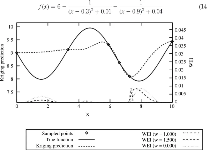
The weighted expected improvement utility function (Sobesteret al., 2005) provides a simple way of controlling the balance between exploration and exploitation, through a real valued parameterw:
WEI½x ¼sðxÞ½wuðxÞFðuðxÞÞ þ ð12wÞfðuðxÞÞ ð12Þ The parameterwtakes values between 0 and 1, withw¼1 placing all the emphasis on the first term on the right hand side of equation (10), i.e. on exploitation, whilstw¼0
Electromagnetic
design
optimization
places all the emphasis on the second term on the right hand side of equation (10), i.e. on exploration. The profile of WEI for different values ofwmay be seen in Figure 2 for the function given in equation (9). It can be seen how the emphasis on searching around the current minimum increases as the value of wincreases, as the maximum of the utility function moves closer to the current minimum.
Finally, it should be noted that other utility functions exist which allow the balance between exploration and exploitation to be controlled, most notably the generalized expected improvement (Schonlauet al., 1998), however, these will not be explored in this paper.
In practice “cooling” schemes (Schonlauet al., 1998) or “cyclic” schemes (Sobester
et al., 2005) are used to vary the parameters of utility functions. These have the effect of varying the parameters such that some iterations of the algorithm are exploratory, whilst some are exploitative. The scheme used in this paper to vary the value ofwin equation (12) is simply:
w¼jsinðiÞj ð13Þ
whereiis the iteration number.
The algorithm then proceeds either for a fixed number of iterations (an overall total of 30devaluations is used as a stopping criterion in this implementation), or until an acceptable solution has been found.
3. Test function results
The proposed algorithm is now tested on a test function, taken from (Matlab, 2004). The function, known as “Humps” is given by:
fðxÞ ¼62 1
ðx20:3Þ2þ0:012
1
[image:7.519.128.459.363.602.2]ðx20:9Þ2þ0:04 ð14Þ
Figure 2.
The weighted expected improvement utility function is shown for three different settings ofw, for the function given in equation (8)
10
9.5
8.5
7.5
Kriging prediction
0 2
Kriging prediction True function Sampled points
WEI (w = 1.500) WEI (w = 1.000)
WEI (w = 0.000)
WEI
4 6
X
8 100
0.005 0.015 0.025 0.035 0.045
0.01 0.02 0.03 0.04
8 9
COMPEL
26,2
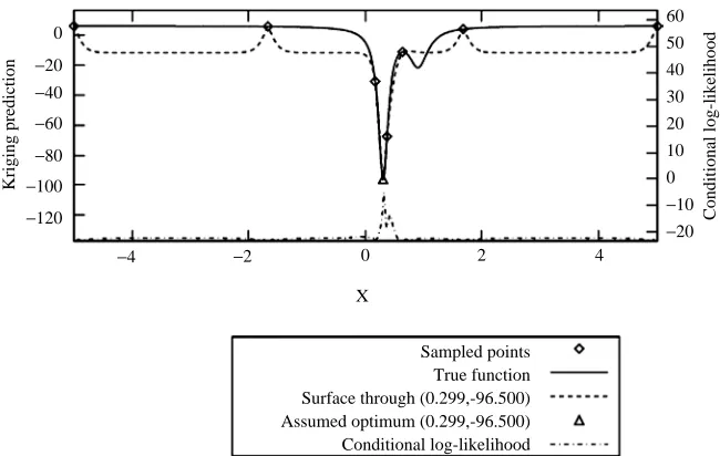
wherex[½25;5. The number of evaluations taken to locate the minimum within 1 percent tolerance was 8. Thus, the optimum was located during step 2 of the algorithm, after just four iterations. The Kriging prediction at the fourth iteration is shown in Figure 3. As can be seen, the Kriging prediction when the optimum is found is not very accurate; however, this should be of no concern. The purpose of optimization is simply to locate the optimal point, not to accurately predict the function being optimized as well. This is related to Vapnik’s (2006) principle from machine learning:
When solving a problem of interest, do not solve a more general problem as an intermediate step. Try to get the answer that you really need but not a more general one.
In the case of optimization, the problem of interest is only to locate the minimum of an unknown function. In particular, we are not concerned with the more general problem of approximating the unknown function as accurately as possible first. Thus, the fact that the Kriging approximation at the fourth iteration is not very accurate (globally) is not an issue: the optimum point has been located regardless.
In this case, it is known that the optimum has been found at the 8th evaluation, and so the algorithm can terminate (i.e. scenario 1 in section 2.3 has arisen). However, in general it is not known if the optimum has been found, and so the algorithm will proceed to step 3. This is precisely what happens in the next example: the optimal design of an electron gun.
4. Application to electromagnetic design problem
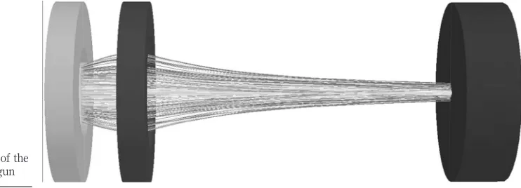
[image:8.519.62.387.395.601.2]The proposed algorithm was applied to an electromagnetic optimal design problem. The voltage on, and position of, the focus electrode of an electron gun was varied so as to focus the beam of electrons on the center of the anode as much as possible. Formally, denoting the voltage on the focus electrode byVvolts, and its perpendicular distance from the emitting surface bydcm, the objective function is:
Figure 3. Iteration 4 for Humps function
Sampled points
Kriging prediction
Conditional log-likelihood Assumed optimum (0.299,-96.500) Surface through (0.299,-96.500) True function X
0
−20
−40
−60
−80
−100
−120
−20
−10 0 10
Conditional log-likelihood
20 30 40 50 60
−4 −2 0 2 4
Electromagnetic
design
optimization
Minimize fðV;dÞ ¼
Z
anode
JðrÞr2dS with V [½0;1000 and d[½5;10 ð15Þ
whereris the radial distance from the center of the anode surface,J(r) is the current density atr, and the integral is taken over the surface of the anode. Each analysis was carried out using the Vector Fields OPERA program, with the space charge solver SCALA. A random search of 100 iterations and a genetic algorithm (of population size ten, and ten generations in length, thus also having 100 iterations in total) were also carried out for comparison.
After 100 iterations of the random search algorithm, the best solution obtained had a value of f¼0.1493, whilst the best solution found by the genetic algorithm had a value off¼0.1349. This was used to set a suitable targetf*for step 2 of the proposed
algorithm, although the method suggested in section 2.2 could also have been used. After just 14 evaluations (still in step 2 of the algorithm) a better solution than the random search was found by the proposed algorithm, with a value of f¼0.1479. Allowing the algorithm to proceed further to step 3, further improvements were made. Using a stopping criteria of 30d (¼60) evaluations in total, the final solution, found during the third step, had an objective function value off¼0.0867.
The configuration of this final design is shown in Figure 4.
5. Conclusions
An algorithm has been proposed which combines for the first time the techniques of two-stage and one-stage selection of points in surrogate model-assisted optimization. Furthermore, it is believed that this is the first time a one-stage method has been used in electromagnetic design optimization.
[image:9.519.88.459.469.603.2]It was found that the proposed method worked well in locating the minimum of a difficult test function, without even constructing an accurate approximation to it. This suggests that surrogate models need not be accurate approximations to the true function in order to locate the minimum, provided they are interpreted and used in an appropriate manner. The algorithm was applied to an electromagnetic design problem, and was found to outperform both a random search (of 100 iterations in length) in just 14 iterations, and a genetic algorithm (also of 100 iterations in length), in 60 iterations.
Figure 4.
Final configuration of the optimized electron gun
COMPEL
26,2
References
Gutmann, H.M. (2001), “A radial basis function method for global optimization”,Journal of Global Optimization, Vol. 19 No. 3, pp. 201-27.
Hawe, G.I. and Sykulski, J.K. (2007), “Considerations of accuracy and uncertainty with Kriging surrogate models in single-objective electromagnetic design optimization”,IET Science, Measurement and Technology, in press.
Jones, D.R. (2001), “A taxonomy of global optimization methods based on response surfaces”, Journal of Global Optimization, Vol. 21, pp. 345-83.
Jones, D.R., Schonlau, M. and Welch, W.J. (1998), “Efficient global optimization of expensive black-box functions”,Journal of Global Optimization, Vol. 13, pp. 455-92.
Kalagnanam, J.R. and Diwekar, U.M. (1997), “An efficient sampling technique for off-line quality control”,Technometrics, Vol. 39 No. 3, pp. 308-19.
Lebensztajn, L., Marretto, C.A.R., Costa, M.C. and Coulomb, J.-L. (2004), “Kriging: a useful tool for electromagnetic devices optimization”,IEEE Transactions on Magnetics, Vol. 40 No. 2, pp. 1196-9.
Locateli, M. (1997), “Bayesian algorithms for one-dimensional global optimization”,Journal of Global Optimization, Vol. 10, pp. 57-76.
Matlab (2004),High-Performance Computation and Visualization Software Reference Guide, The MathWorks Inc., Natick, MA.
Nelder, J.A. and Mead, R. (1965), “A simplex method for function minimization”, Computer Journal, Vol. 7, pp. 308-13.
Santner, T.J., Williams, B. and Notz, W. (2003), The Design and Analysis of Computer Experiments, Springer-Verlag, New York, NY.
Sasena, M.J. (2002), “Flexibility and efficency enhancements for constrained global design optimization with Kriging approximations”, PhD dissertation, University of Michigan, Ann Arbor, MI.
Sasena, M.J., Papalambros, P. and Goovaerts, P. (2002), “Exploration of metamodelling sampling criteria for constrained global optimization”,Engineering Optimization, Vol. 34, pp. 263-78. Schonlau, M., Welch, W.J. and Jones, D.R. (1998), “Global versus local search in constrained optimization of computer models”, IMS Lecture Notes, Institute of Mathematical Statistics, Beachwood, OH.
Sobester, A., Leary, S.J. and Keane, A.J. (2005), “On the design of optimization strategies based on global response surface approximation models”,Journal of Global Optimization, Vol. 33, pp. 31-59.
Vapnik, V. (2006),Estimation of Dependences Based on Empirical Data, 2nd ed., Springer-Verlag, New York, NY.
Further reading
Dixon, L.C.W. and Szego¨, G.P. (1978), “The global optimization problem: an introduction”, Towards Global Optimisation 2, North-Holland Publishing Company, Amsterdam.
About the authors
Glenn Hawe graduated in 2004 from the University of Warwick with a Masters degree in Mathematics and Physics. He is currently a KTP Associate working with Vector Fields Ltd, Oxford and the School of Electronics and Computer Science at the University of Southampton. He is registered at the university as a part-time PhD student, where his research area is
Electromagnetic
design
optimization
cost-effective optimization techniques. Glenn Hawe is the corresponding author and can be contacted at: [email protected]
Jan Sykulski is a Professor of Applied Electromagnetics and Head of Electrical Power Engineering Group of the School of Electronics and Computer Science at the University of Southampton. His research interests are in the areas of power applications of high temperature superconductivity, modelling of superconducting materials, advances in simulations of coupled field systems, development of fundamental methods of computational electromagnetics and new concepts in design and optimization of electromechanical devices. He has 224 publications listed on the official database of the University. He is a founding Secretary/Treasurer/Editor of International Compumag society, a Visiting Professor at universities in Canada, Italy, Poland, France and China, a founding member of International Steering Committees of major international conferences, including COMPUMAG, IEEE CEFC, IEE CEM, ISEF, EPNC and others. He is Fellow of IEE, Institute of Physics and British Computer Society.
COMPEL
26,2
246
To purchase reprints of this article please e-mail:[email protected]