https://doi.org/10.1007/s10921-018-0501-5
Wave Interaction with Defects in Pressurised Composite Structures
R. K. Apalowo1·D. Chronopoulos1·G. Tanner2
Received: 23 January 2017 / Accepted: 13 June 2018 © The Author(s) 2018
Abstract
There exists a great variety of structural failure modes which must be frequently inspected to ensure continuous structural integrity of composite structures. This work presents a finite element (FE) based method for calculating wave interaction with damage within structures of arbitrary layering and geometric complexity. The principal novelty is the investigation of pre-stress effect on wave propagation and scattering in layered structures. A wave finite element (WFE) method, which combines FE analysis with periodic structure theory (PST), is used to predict the wave propagation properties along periodic waveguides of the structural system. This is then coupled to the full FE model of a coupling joint within which structural damage is modelled, in order to quantify wave interaction coefficients through the joint. Pre-stress impact is quantified by comparison of results under pressurised and non-pressurised scenarios. The results show that including these pressurisation effects in calculations is essential. This is of specific relevance to aircraft structures being intensely pressurised while on air. Numerical case studies are exhibited for different forms of damage type. The exhibited results are validated against available analytical and experimental results.
Keywords Composite structures·Pressurisation·Wave finite element·Wave interaction with damage·Wave propagation
Nomenclature
+,− Positive and negative going waves properties a Wave amplitude
c Wave scattering coefficient
D,D Dynamic stiffness matrices of the waveguide and the coupling joint
k Wavenumber
K,M,C Stiffness, mass and damping matrices of a waveguide’s modelled periodic segment q,f Physical displacement and forcing vectors
for an elastic waveguide S Wave scattering matrix
T Wave propagation transfer matrix
z Physical displacement vector for the cou-pling joint
φ,Φ Eigenvector and grouped eigenvector Matrix transpose
B
R. K. Apalowo1 Institute for Aerospace Technology & The Composites
Research Group, The University of Nottingham, NG7 2RD Nottingham, UK
2 School of Mathematical Sciences, University of Nottingham,
University Park, NG7 2RD Nottingham, UK
λ Propagation constant and eigenvalue of the wave propagation eigenproblem
i,n Property of interface and non-interface nodes
J Property of a coupling joint
K,M,C Stiffness, mass and damping stiffness matri-ces of the coupling joint
ω Angular frequency
Real operator
b,h Width and depth of a cross-section
E,G, ν, ρ Elastic modulus, shear modulus, Poisson’s ratio and density of an elastic waveguide
g Global coordinate index
j Number of DoFs on each cross-section of the periodic waveguide segment
k,n,N Waveguide indices and total number of waveguides existing in the considered sys-tem
L Length
L,R,I Left, right sides and interior indices
q,f Displacement and forcing indices
s Periodic segment positioning index
t Time
w,W Wave eigenvector index and total number of waves accounted for in the waveguide
1 Introduction
Composite structures are increasingly used in modern aerospace and automobile industries due to their well-known benefits. However, they exhibit a wide range of structural failure modes, which include delamination, notch, crack, fibre breakage and fibre-matrix debonding [1], for which the structures have to be frequently and thoroughly inspected in order to ensure continuous structural integrity. Approxi-mately, 27% of an average modern aircraft’s lifecycle cost [2] is dedicated on inspection and repair. The use of ’offline’ structural inspection techniques currently leads to a massive reduction of the aircraft’s availability and significant financial losses for the operator. Structural health monitoring (SHM) combines non-destructive evaluation (NDE) technologies with new modelling methodologies and robust sensing tech-nologies to detect, identify and monitor the integrity of structures and predict their remaining lifetime. The non-destructive detection and evaluation of damage in industrial structural components during service, is of pertinent impor-tance for monitoring their condition and estimating residual life. This evaluation has been widely studied using the ultra-sonic guided wave techniques. These techniques are more sensitive to gross defects compared to micro damage. How-ever, acousto-ultrasonic techniques [3,4], which are excellent for both forms of defects, have been receiving increasing attention during the last decade.
Non-destructive ultrasonic wave distortion during prop-agation in structural media has been studied as early as in [5]. It has been demonstrated that ultrasonic waves can be successfully employed in non-destructive detection of struc-tural defects and deterioration (such as fatigue) [6–8]. The developed NDE approaches can be classified into matrix for-mulation techniques: in which ultrasonic waves in layered media are defined by coupling the matrix formulation of each of the layers which constitute the media, and wave propaga-tion techniques: which strongly rely on the calculapropaga-tion of dispersion curves and wave interaction reflection and trans-mission coefficients to inspect and evaluate structural media. The wave propagation NDE inspection techniques can fur-thermore be categorised into two steps, namely response and modal steps [9]. The former measures the wave reflection and transmission characteristics of the structure, while the latter determines the wave dispersion and propagation char-acteristics, such as the wave phase and group velocities as well as the wavenumber. These techniques have been suc-cessfully demonstrated in various structural media such as truss [10,11], beams [12], 3-D solid media [13] and compos-ite structure [14]. It has also been applied to calculate wave interaction coefficients from structural joints such as curved [15], spring-type [16], welded [2], adhesive [17], angled [18] and liquid-coupled joints [19].
Implementing a suitable modelling technique is as impor-tant as selecting an appropriate NDE method for SHM. The finite element (FE) method [20] is one of the most common ones employed to analyse the dynamic behaviour of struc-tures. The structure is split into a number of elements to form a mesh and equilibrium relationships which are applied to relate the entire structure and boundary conditions to arrive at a unique solution for a specific problem. Finite element based wave propagation NDE technique for periodic struc-tures was first introduced in [21]. It was shown that the wave dispersion characteristics within the layered media can be accurately predicted for a wide frequency range by solving an eigenvalue problem for the wave propagation constants. The work was extended to 2-D media in [22]. The wave finite element (WFE) method was introduced in [23] to facil-itate the post-processing of the eigenvalue problem solutions and the improvement of the computational efficiency of the method was presented in [24]. The method is considered as an expansion of Bloch’s theorem and its main assump-tion being the periodicity of the structure to be modelled. It couples the periodic structure theory to the FE method by modelling only a small periodic segment of the struc-ture, thereby saving a whole lot of computational cost and time. WFE method has been successfully implemented in 1-D [23,25] and 2-D [26,27] wave propagation analyses. The method has recently found applications in predicting the vibroacoustic and dynamic performance of layered struc-tures [28]. The variability of acoustic transmission through layered structures [29,30], as well as structural identifica-tion [31] have been modelled through the same methodology. The same FE based approach was employed to compute the reflection and transmission coefficients of waves impinging on linear joints in [25,32].
Fig. 1 Internal (core) pressurisation of a periodic segment of a sandwich structure
2 Stiffness Property of a Pressurised
Structure
Pre-stress impact (due to pressurisation) on the coefficients of wave interaction with defects is examined in this work. Consider an arbitrary periodic segment internally pressurised as shown in Fig.1. The stress stiffening effect as a result of the applied pressure is accounted for by adding a pre-stress stiffness matrix,Kp, to the unstressed stiffness matrix,K0,
of the system.
Kpis dependent on the geometry, displacement field and
the state of stress of each structural element [33]. For a 3-D element, which is considered in this work, the pre-stress stiffness matrix is given as [34]
Kp=
SgSmSgdxdydz (1)
whereSgis the shape function derivative matrix,Sm is the
Cauchy stress tensor and[•]is a transpose. Hence, the total stiffness matrix of the pre-stressed system is given as
K=K0+Kp (2)
Evidently,Kequals toK0under no pressurisation scenario.
3 Finite Element Modelling of Structural
Damage
A system of N waveguides connected through a coupling joint (Fig.4) is considered in this study. In the general case, waves travel from one of the waveguides to other waveguides
through the joint. Scattering coefficients are calculated from interaction of the waves with structural inconsistencies (such as damage). Composite structures are prone to a number of structural failure modes which range from microscopic fibre faults to large, gross impact damage. Among these failure modes, notch, cracks, delamination and fibre breakage are important modes of failures commonly found in composites [1,35].
Simplified FE methods can be used to simulate the effect of the damage on the mechanical behaviour of the cou-pling joint. Some of these methods include element deletion, stiffness reduction, duplicate node and kinematics based methods. Descriptions of each of these methods and their applicability are given in the following sections.
3.1 Element Deletion Method
This method is mainly applicable for modelling notches such as holes (fibre fractures) and rectangular notches in compos-ites. Here, an element or a number of elements along the axis of the defect is/are deleted from the structure to simulate the effect of the defect. This leads to a reduction in the overall mass and stiffness of the structure. It is one of the simplest FE damage modelling methods as it doesn’t require mesh modification.
3.2 Stiffness Reduction Method
It is a known fact that structural defects contribute to a reduction in the overall stiffness properties of the structural segment. In this method, the stiffness loss is incorporated in the FE modelling of the structure by multiplying the material property of the structure by a reduction factorβ as
P=βP0, 0< β≤1 (3)
where P is the reduced material property, P0 the original
magnitude of the property (which can be elastic modulus, shear modulus or density). β being the reduction factor, equals unity for a pristine structure. This method is applicable to model cracks and delamination, but it is limited to wave interaction problem where mode conversion is not expected.
3.3 Node Duplication Method
The node duplication method is applicable for modelling var-ious damage types such as single and multiple delamination and cracks, and fibre breakages.
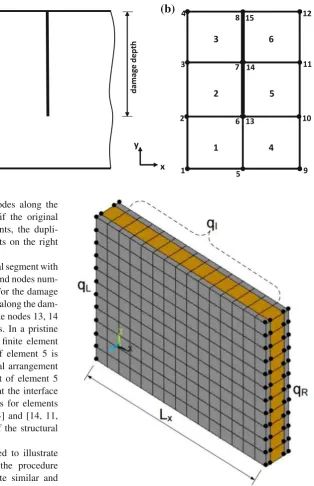
Fig. 2 Finite element modelling of damage using node
duplication method:adamaged structural segment,bnode duplication model
(
a
)
(b)
that when a tensile force is applied, the nodes along the crack front are separated. In this respect, if the original nodes are connected to the left side elements, the dupli-cate nodes will be connected to the elements on the right side.
As an illustration of this method, a structural segment with six plane strain FEs is considered. Elements and nodes num-bering of the segment are as shown Fig.2. For the damage depth considered, nodes 6, 7 and 8, which are along the dam-age axis, are disconnected by adding duplicate nodes 13, 14 and 15 of same respective nodal coordinates. In a pristine state of the segment, nodal arrangement of finite element 2 is [2, 6, 7, 3] in that order, while that of element 5 is [6, 10, 11, 7]. But, in a damaged state, nodal arrangement of element 2 remains [2, 6, 7, 3] while that of element 5 becomes [13, 10, 11, 14] to model defects at the interface of the two FEs. Similar node ordering holds for elements 3 and 6 with nodal arrangements [3, 7, 8, 4] and [14, 11, 12, 15] respectively in the damaged state of the structural segment.
Although a 2D structural segment is used to illustrate the procedure of this method, extending the procedure to model damage in a 3D structure is quite similar and straightforward.
3.4 Kinematics Based Method
This approach has a lot of similarities to the node duplication method. It involves enforcing kinematics to the nodes sur-rounding the damage. The structural segment is segmented into multiple domains along the crack front. The stiffness and mass matrices of each domain are generated and coupled to obtain the overall matrices of the structural segment. More details on the approach can be found in [36]. The method is applicable to model delamination, cracks and fibre break-ages.
Fig. 3 WFE modelled layered composite waveguide with the left and right side nodesqL,qRbullet marked. The range of interior nodesqI also illustrated
4 Free Wave Propagation in an Arbitrarily
Periodic Structure by WFE Method
Linear elastic wave propagation is considered in thex direc-tion of the arbitrary periodic structural waveguide of Fig.3. A FE model, of a periodic segment of the structural waveguide, is meshed using commercial FEA software.
[image:4.595.231.546.54.541.2]stiff-ness matrix (DSM),D, which relates the nodal displacements and the internal forces (of the periodic segment’s nodes) under a time-harmonic behaviour assumption, is given as
[K+iωC−ω2M]q=f (4)
whereqandf are the displacement and internal force vec-tors respectively.CandMare respectively the damping and mass matrices of the segment. The internal force vector is responsible for transmitting waves from one element to the other within the structure, hence it is not zero, even for a free wave motion where no external load is applied [27], as is the case being considered in this work.
The DSM can be partitioned with regards to the left L, rightRand internalI DoFs of the periodic segment as
⎡
⎣DDLLIL DDLIII DDLRIR
DRLDRIDRR ⎤ ⎦
⎧ ⎨ ⎩
qL
qI
qR ⎫ ⎬
⎭=
⎧ ⎨ ⎩
fL
fI
fR ⎫ ⎬
⎭ (5)
Using a dynamic condensation technique for the internal nodes DoFs, Eq. (5) can be expressed in the form
DLL−DLID−II1DIL DLR−DLID−II1DIR
DRL−DRID−II1DILDRR−DRID−II1DIR
qL
qR
=
fL
fR
(6)
As earlier stated, it is assumed that no external forces are applied on the segment. As a result of this, the displacement continuity and equilibrium of forces equations at the interface of two consecutive periodic segmentssands+1 are given as
qsR =qsL+1
fRs = −fLs+1 (7)
The transfer matrix,T, relates the displacement and force vectors of the left and right sides of the periodic segments. This is done by combining Eqs. (6) and (7) as
qLs+1 fLs+1
=T
qsL fLs
(8)
and the expression for the symplectic transfer matrix is defined as
T =
D11 D12
D21 D22
(9)
with
D11= −(DLR−DLID−II1DIR)−1(DLL−DLID−II1DIL)
D12=(DLR−DLID−II1DIR)−1
D21=(−DRL+DRID−II1DIL)+(DRR+DRID−II1DIR)
×(DLR−DLID−II1DIR)−1(DLL−DLID−II1DIL)
D22= −(DRR+DRID−II1DIR)(DLR−DLID−II1DIR)−1
(10)
With a wave propagating freely along the x-direction (1-dimensional wave propagation), the propagation constant,
λ = e−i k Lx, relates the left and right nodal displacements and forces by
qsR=λqsL
fRs = −λfLs (11)
By substituting Eqs. (7) and (11) in Eq. (8), the free wave propagation is described by the eigenproblem relation
λ
qsL fLs
=T
qsL fLs
(12)
whose eigenvalues λω and eigenvectors φω = λ
φq
φf
ω solution sets provide a comprehensive description of the propagation constants and the wave mode shapes for each of the elastic waves propagating in the structural waveguide at a specified angular frequencyω. Both positive going (with
λ+
ω andφ+ω) and negative going (withλ−ω andφ−ω) waves are sought through the eigensolution. Positive going waves are characterised [23] by
|λ+ω| ≤1
(iωφ+fφq+) <0 if|λ+ω| =1 (13)
which states that when a wave is propagating in the positive
xdirection, its amplitude should be decreasing, or that if its amplitude is constant (in the case of propagating waves with no attenuation), then there is time average power transmis-sion in the positive direction. Then the wavenumbers of the waves (at a specified angular frequency) in the positivek+ω and the negativek−ω directions can be determined from the propagation constants as
k+ω = −ln(λ + ω)
i Lx
k−ω = −ln(λ − ω)
i Lx
Fig. 4 Periodic elastic waveguides connected through a coupling joint. Waves having amplitudesa+n impinging on the joint from thenth waveguide will give rise to waves of reflection coefficientscn,nin the nth waveguide and waves of transmission coefficientsck,nin thekth waveguide
5 Elastic Wave Interaction Modelling by
Hybrid WFE-FE Approach
In the general case, a system ofN healthy periodic waveg-uides connected through a structural coupling joint as shown in Fig. 4 is considered. The coupling joint could exhibit arbitrarily complex mechanical behaviour such as damage, geometric or material inconsistencies and is fully FE mod-elled. As already stated, each waveguide can be of different and arbitrary layering and can also support a number (W) of propagating waves at a given frequency.
Propagation constants of the waves are sought through the WFE methodology as presented in Sect.4. Each supported wavemode w with w ∈ [1· · · W] for waveguide n with
n∈ [1· · · N]in the system can be grouped as
+ n,q =
φ+q,1 φ+q,2 · · · φ+q,W
+n,f =
φ+f,1 φ+f,2 · · · φ+f,W
− n,q =
φ−q,1 φ−q,2 · · · φ−q,W
−n,f =φ−f,1 φ−f,2 · · · φ−f,W
(15)
with each matrix being of dimension [j ×W]. The wave-modes of the entire system can be computed at each specified angular frequency and be grouped as
+
q =
⎡ ⎢ ⎢ ⎢ ⎢ ⎢ ⎣
+1,q 0 · · · 0
0 +2,q · · · 0
· · · ·
0 0 · · · +N,q
⎤ ⎥ ⎥ ⎥ ⎥ ⎥ ⎦
[j N×W N]
(16)
with respective similar expressions for+f ,−q and−f . A local coordinate system is defined for each waveguide such that the waveguide’s positive axis is directed towards the joint. The rotation matrixRn transforms the DoFs of each
waveguide from the local to the global coordinates of the system as
g,+
q =R+q (17)
with respective similar expressions forgf,+,qg,−andgf,−.
g denotes the global coordinates index andRrepresents the rotation matrices of the system’s waveguides, grouped in a block diagonal matrix as
R =
⎡ ⎢ ⎢ ⎣
R1 0 · · · 0
0 R2 · · · 0
· · · ·
0 0 · · · RN
⎤ ⎥ ⎥ ⎦
[j N×j N]
(18)
The equation of motion for the FE modelled coupling joint can be in general written as
M¨z(t)+C˙z(t)+Kz(t)=fe(t) (19)
with the frequency dependent DSM of the joint expressed as
D=K+iωC−ω2M (20)
whereK,CandMare stiffness, damping and mass matrices of the coupling joint,zis the physical displacement vector of the coupling joint andfeis the set of elastic forces applied to
[image:6.595.198.544.56.278.2]to be purely elastic and that no external force is applied at the non-interface nodes of the joint. As a result of this and similar to the waveguides, the DSM of the joint can be partitioned with regards to the interfaceiand non-interfacennodes of the joint with the waveguides as
Dii Din DniDnn
zi zn
=
fe
0
(21)
Using a dynamic condensation for the non-interface DoFs, Eq. (21) can be expressed as
DJzi(t)=fe(t) (22)
with
DJ=Dii−DinD−nn1Dni (23)
whereDJis of dimension [j N×W N].
The equilibrium of forces at the coupling joint gives
fe(t)−Rf(t)=0 (24)
wheref is the set of forces applied by the waveguides con-nected to the joint and the continuity conditions for the joint give
zi(t)=Rq(t) (25)
with
q= [q1 q2 · · ·qN][jN×1] (26)
Waves of amplitudesan+are impinging on the coupling
joint from thenth waveguide. These give rise to reflected waves of amplitudesan−in thenth waveguide and transmitted waves of amplitudesa−k in thekth waveguide (and vice versa as shown in Fig.4) expressed as
a−n =cn,na+n
a−k =ck,na+n
(27)
withcn,n and ck,n respectively being matrices containing
the reflection and transmission coefficients of the scattered waves. Hence, the incident waves amplitudes can be related to the amplitudes of the scattered waves as
a−=Sa+ (28)
where a[+WN×1] is the vector containing the amplitudes of the incident waves moving towards the coupling joint and a−[WN×1]the vector containing the amplitudes of the reflected and transmitted scattered waves. The wave scattering matrix
S whose diagonal and off-diagonal elements respectively represent the reflection and transmission coefficients of the scattered waves can be expressed in the form
S =
⎡ ⎢ ⎢ ⎢ ⎢ ⎣
c1,1 · · · c1,W · · · c1,WN
· · · ·
cW,1 · · · cW,W · · · cW,WN
· · · ·
cWN,1 · · · cWN,W · · · cWN,WN
⎤ ⎥ ⎥ ⎥ ⎥ ⎦
[W N×W N]
(29)
A transformation can be defined for the motion in the waveguides between the physical domain, where the motion is described in terms ofq(t)andf(t)and the wave domain, where the motion is described in terms of waves of ampli-tudes a+ and a− travelling in the positive and negative directions respectively as
qn(t)=+n,qan+cos(ωt)+−n,qan−cos(ωt)
fn(t)=+n,fa+n cos(ωt)+−n,fan−cos(ωt)
(30)
and by concatenating the corresponding vectors and matrices, the general expressions for q(t)andf(t)for the system’s waveguides can be expressed as
q(t)=+qa+n cos(ωt)+−qa−n cos(ωt)
f(t)=+fa+n cos(ωt)+−fa−n cos(ωt) (31)
Substituting Eq. (22) into the equilibrium equation (Eq. (24)) and then substitute the continuity equation (Eq. (25)) into the resulting expression gives
DJRq=Rf (32)
Substituting Eqs. (17) and (31) in Eq. (32) and express the resulting equation in the form of Eq. (28) gives the wave interaction scattering matrix as
S= −[gf,−−DJgq,−]−1[gf,+−DJgq,+] (33)
6 Numerical Case Studies
Fig. 5 Two bars connected through another bar (coupling joint)
cases present the application of the proposed scheme in com-puting waves propagation constants and quantifying waves interaction with defects within damaged layered structures subjected to pressurisation. Effect of pre-stress (due to pres-surisation) on these waves properties is also examined. In all cases, finite element size is chosen to ensure that mesh density is fine enough to represent the structure accurately at a reasonable computational cost. All properties and dimen-sions are in SI units, unless otherwise stated.
6.1 Validation Case Studies
6.1.1 Two Collinear Bars Coupled Through a Finite Bar
Two collinear bars connected through another bar (the coupling joint) of a different material characteristics is con-sidered. The bars are of uniform circular cross-section and undergo longitudinal vibration. Arrangement of the bars is presented in Fig.5. Each waveguide is made of aluminium (E1 = E2 =70×109,ρ1 = ρ2 = 2600) and the joint is
made of steel (EJ =210×109,ρJ =7500). Cross-sectional
areasA1=A2=AJ =0.003, lengthsL1=L2=0.2 and LJ =0.003.
Incident wave of amplitudea+1 impinging on the coupling joint from waveguide 1 will give rise to reflected and trans-mitted waves of amplitudesa−1 anda2+in waveguides 1 and 2 respectively. Standing wave is present in the joint since both forward and backward moving waves of amplitudesaJ+and a−J are simultaneously present.
Imposing necessary boundary conditions across the cou-pling joint gives the transfer function of the waves as [15]
B a1−a+J a−J a2+=1k1E1A10 0
a+1 (34)
with
B= ⎡ ⎢ ⎢ ⎣
−1 1 1 0
k1E1A1 kJEJAJ −kJEJAJ 0
0 e−i kJL ei kJL −e−i k2L 0 −kJEJAJe−i kJL kJEJAJei kJL k2E2A2e−i k2L
⎤ ⎥ ⎥ ⎦
(35)
Frequency [kHz]
0 50 100 150 200 250 300 350 400
Wavenumber [1/m]
0 100 200 300 400 500
Fig. 6 Dispersion curves for the longitudinal wave in the bar: Analytical(-), WFE(- -)
where kn are longitudinal wavenumbers of the bars
deter-mined at each considered frequencyωas
kn=ω
ρ
n En
n∈ [1,2,J] (36)
Equation (34) is solved for the reflectionc11 (witha1− =
c11a1+) and transmissionc21(witha2+=c21a1+) coefficients
of the system.
The methodology presented in this work is used to com-pute the numerical solution of the problem. A segment of each waveguide is modelled using LINK180 FE of length
Δ = 0.001 in ANSYS. The coupling joint is modelled using three finite elements of similar element size as the waveguides. Then Eq. (12) is solved to obtain the WFE wave dispersion properties. Equation (33) is solved for the WFE/FE wave interaction coefficients. Comparison of the presented WFE/FE predictions and the analytical results are presented in Figs.6and7respectively. Excellent agreements are observed in the results. Correlation of the transmission coefficient results is good but with little deviation at higher frequencies. This is as a result of FE discretisation whose accuracy limit is recommended to satisfy [37]
[image:8.595.124.536.53.341.2]Fig. 7 Wave interaction coefficients for two collinear bars coupled through a finite bar: analytical(-), WFE-FE(- -). aReflection coefficient.b Transmission coefficient
Frequency [kHz]
0 50 100 150 200 250 300 350 400
Magnitude
0 0.1 0.2 0.3 0.4 0.5
Frequency [kHz]
0 50 100 150 200 250 300 350 400
Magnitude
0.86 0.88 0.9 0.92 0.94 0.96 0.98 1
(a) (b)
Fig. 8 Schematic illustration of a delaminated beam discretised as a system of two healthy beams connected through a delaminated beam (coupling joint)
As a result of this, for a particular element size Δ, FE discretisation error increases with frequency because wavenumber increases as frequency increases (as shown in Fig.6). Hence, the deviation observed at higher frequencies between the numerical and analytical results can be attributed to FE discretisation error. This error can be subdued using smaller element sizeΔbut at a higher computational cost.
6.1.2 Delaminated Beam
The presented methodology is next validated using delami-nated continuous aluminium beam having a uniform cross-sectional area withL1=L2=0.2,LJ =0.001,b=0.003
andh=0.001. The beam is made of aluminium with mate-rial propertiesE =70×109,ρ =2600 andν =0.3. The continuous beam is discretised as a system of two healthy waveguides connected through a delaminated coupling joint as shown in Fig.8. The beam supports propagating longitu-dinal, in-plane bending, out-of-plane bending and torsional waves.
A segment of each waveguide is modelled using SOLID185 finite element of lengthΔ=0.001 in ANSYS. The coupling joint is modelled using similar segment length as the waveguides. The through width delamination in the coupling joint is modelled using the stiffness reduction method (Sect.3.2) with a reduction factorβ =0.01. Equa-tion (12) is solved to obtain the WFE wave dispersion properties. Then the WFE-FE reflection and transmission efficiencies are calculated as the absolute square of the reflec-tion and transmission coefficients obtained through Eq. (33).
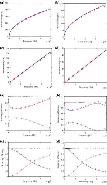
Waves dispersion properties, and reflection and transmis-sion efficiencies of the system are obtained analytically as in [15,38]. These are compared to the WFE/FE predicted results as shown in Figs.9and10. The analytical and numerical pre-dictions are in very good agreement.
The coupling joint is undamped, i.e. it is of real-valued elastic and shear moduli. As a conservation of energy con-dition, the algebraic sum of reflection and transmission efficiencies of a lossless (undamped) structural segment equals unity. As observed in Fig.10, conservation of energy condition is satisfied for all presented waves as sums of reflection and transmission efficiencies are ones. This further establishes the validity of the presented methodology. Also observed in the waves transmission and reflection results is the fact that the incident waves in waveguide 1 is transmitted or reflected through the coupling joint into waves of the same type without any form of mode conversion. This is expected in waveguides collinearly connected through a joint as waves will be fully transmitted without reflection and modes con-version. Reflection observed is solely as a result of damage in the coupling joint.
6.1.3 Notched Plate
Validity of the presented methodology is further proven using notched plate of thickness 2d=0.003 and lengthL =0.6. The plate is made of mild steel (E =210×109,ρ=7850 andν = 0.29) and has uniform area throughout its cross sections.
Based on the presented methodology, the plate can be discretised as a system of two pristine waveguides (L1 = L2 = 0.295) connected through a notched coupling joint
(LJ = 0.01) as shown in Fig.11. Plane strain condition is
assumed.
[image:9.595.172.544.56.184.2]Fig. 9 Dispersion curves for the beam: Present methodology (-) and Analytical results (o).a Bending wave about y-axis.b Bending wave about z-axis.c Torsional wave.dLongitudinal wave
× ×
Frequency [Hz] 104
0 1 2 3 4
Wavenumber [1/m]
0 100 200 300 400 500
Frequency [Hz] ×
× 104
4
Wavenumber [1/m]
0 50 100 150 200 250
Frequency [Hz] 104
0 1 2 3 4
Wavenumber [1/m]
0 20 40 60 80 100 120 140
Frequency [Hz] 104
0 1 2 3
0 1 2 3 4
Wavenumber [1/m]
0 10 20 30 40 50
(
a
)
(b)
(c)
(
d
)
Fig. 10 Reflection and transmission efficiencies of the delaminated beam joint. Present methodology: reflection (o), transmission (∗). Analytical results: reflection (- -), transmission (-). Conservation of energy (. . .).aBending wave about y-axis.bBending wave about z-axis.cTorsional wave. dLongitudinal wave
Frequency [Hz] 104
Scattering efficiency
0 0.2 0.4 0.6 0.8 1
Frequency [Hz] ×
× ×
× 104
Scattering efficiency
0 0.2 0.4 0.6 0.8 1 1.2
Frequency [Hz] 104
0 1 2 3 4
0 1 2 3 4
Scattering efficiency
0 0.2 0.4 0.6 0.8 1 1.2
Frequency [Hz] 104
0 1 2 3 4
0 1 2 3 4
Scattering efficiency
0 0.2 0.4 0.6 0.8 1 1.2
(
a
)
(b)
[image:10.595.183.541.55.671.2]Fig. 11 Schematic illustration of a notched plate discretised as a system of two healthy waveguides connected through a notched coupling joint
Waves reflections are obtained from notches, of depths 0.0005, 0.001 and 0.002, which are respectively 17, 33 and 67% of the plate thickness. Uniform notch (of width 0.0005) is used in all cases. The notches are modelled using the ele-ment deletion approach presented in3.1.
In practice, the wave reflection calculation can be made by a full FE transient simulation. The WFE computed eigen-vectors can be windowed and then applied as time-dependent harmonic displacement boundary conditions (of excitation frequencyω) at one of the extreme cross-sections of the plate. In this case, the entire plate is modelled as one plate instead of a system of waveguides and coupling joint as in the case of the presented WFE-FE approach.
Results obtained through the WFE-FE methodology are compared with that of the full FE transient simulation and the experimental measurements presented in [39]. Modelling parameters used for the WFE/FE methodology are chosen to match those used for the full FE simulation and the experi-mental measurements in [39].
Good agreement is observed among the WFE-FE, full FE and experimental results as shown in Fig.12. It is also wor-thy to state that the developed methodology is more efficient (than the full FE approach) for predicting wave scattering (reflection and transmission) from damage within structural waveguides for the following noted reasons. First, model size and computational time. Finite element mesh of the plate consists of 7200 elements and 15,626 DoFs in the full FE model against a total of 144 elements (12 for each waveg-uide and 120 for the joint) and 390 DoFs in the presented WFE-FE model. Solving the full FE model requires a com-putational time of about 105 min compared to the WFE-FE model which is solved under 5 min. Therefore, a great deal of computational time and hence cost is saved by the WFE-FE approach. Another noted point is in terms of the complex-ity of the structural system. Full FE model mostly assume plane strain condition in order to simplify and reduce model size of a structural system. In this manner, some propagating waves especially those along the suppressed axis might not be captured. However, the presented WFE/FE approach can be applied for analysing wave interaction in complex struc-tural systems (such as composite structures and strucstruc-tural networks) with low computational size and cost.
Frequency (MHz)
Reflection coefficient magnitude
0 0.2 0.4 0.6 0.8 1
Frequency (MHz)
Reflection coefficient magnitude
0 0.2 0.4 0.6 0.8 1
Frequency (MHz)
0.3 0.35 0.4 0.45 0.5 0.55 0.6
0.3 0.35 0.4 0.45 0.5 0.55 0.6
0.3 0.35 0.4 0.45 0.5 0.55 0.6
Reflection coefficient magnitude
0 0.2 0.4 0.6 0.8 1 (a)
(b)
[image:11.595.309.541.56.472.2](c)
Fig. 12 Comparison of the wave reflection coefficients from notch of varying depths: Presented WFE-FE methodology (-), Full FE predic-tions (- -) and Experimental measurements (◦) in [39].a67% notch depth.b33% notch depth.c17% notch depth
6.2 Test Case Studies
6.2.1 Transversely-Isotropic Beam
In this example, a cracked transversely-isotropic laminate having a uniform cross-sectional area (b = 0.01 andh =
0.005) is considered. The beam is defined as a system of two pristine beams (L1 = L2 = 0.2) connected through
a cracked beam (LJ = 0.004) as shown in Fig.13. Each
beam comprises five layers of glass-epoxy whose material properties are Ex = Ey = 68×109, Ez = 40×109, Gx y = 3.6×10⁹,Gyz = Gx z = 1.2×10⁹,νx y = 0.25,
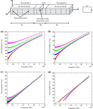
Fig. 13 Schematic illustration of the WFE-FE configuration of a pressurised
transversely-isotropic laminated beam
Fig. 14 Dispersion curves for the transversely-isotropic beam: non-pressurised (-), internal pressurep=0.1 GPa (-+), 0.5 GPa (-x), 1.0 GPa (-*) and 1.5 GPa (-o).aBending wave about y-axis.bBending wave about z-axis.cLongitudinal wave.d Torsional wave
Frequency [Hz] 104 5
Wavenumber [1/m]
0 20 40 60 80 100 120 140 160 180 200
Frequency [Hz] ×
× ×
× 104
5
Wavenumber [1/m]
0 20 40 60 80 100 120 140
Frequency [Hz] 104
0 0.5 1 1.5 2 2.5 3 3.
0 0.5 1 1.5 2 2.5 3 3.5
Wavenumber [1/m]
0 5 10 15 20 25 30 35 40 45
Frequency [Hz] 104
0 0.5 1 1.5 2 2.5 3 3.
0 0.5 1 1.5 2 2.5 3 3.5
Wavenumber [1/m]
0 10 20 30 40 50 60 70 80 90 100
(a) (b)
(c) (d)
A segment (of length Δ = 0.001) of each waveguide is modelled in ANSYS with 40 SOLID185 finite elements using cubed sized elements of length 0.001. Using similar element size, the coupling joint is modelled with 160 finite elements. The crack within the joint is modelled using the node duplication approach (Sect.3.3). Two crack scenarios, of depths 0.001 and 0.002, are considered. These are respec-tively equivalent to 20 and 40% of the total depth of the beam. The cracks are through-width and located at mid length of the joint.
Each beam is pre-stressed using uniform internal pressure. The pressure is applied across the surfaces of the three inter-nal layers of the laminated beam as shown in Fig.13. Five different pressure scenarios are considered; non-pressurised case and pressurised cases with applied pressure p = 0.1 GPa, 0.5 GPa, 1.0 GPa and 1.5 GPa.
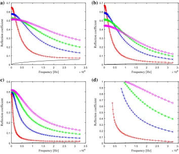
reduc-Fig. 15 Wave reflection coefficients for the
transversely-isotropic laminate with 20% depth crack: non-pressurised (-), internal pressurep=0.1 GPa (-+), 0.5 GPa (-x), 1.0 GPa (-*) and 1.5 GPa (-o).aBending wave about y-axis.bBending wave about z-axis.cLongitudinal wave.d Torsional wave
Frequency [Hz] 104
5
Reflection coefficient
0 0.1 0.2 0.3 0.4 0.5 0.6 0.7
Frequency [Hz] ×
× ×
× 104
5
Reflection coefficient
0 0.1 0.2 0.3 0.4 0.5 0.6 0.7
Frequency [Hz] 104
0 0.5 1 1.5 2 2.5 3 3.
0 0.5 1 1.5 2 2.5 3 3.5
Reflection coefficient
0 0.1 0.2 0.3 0.4 0.5 0.6
Frequency [Hz] 104
0 0.5 1 1.5 2 2.5 3 3.
0 0.5 1 1.5 2 2.5 3 3.5
Reflection coefficient
0 0.1 0.2 0.3 0.4 0.5 0.6 0.7 0.8 0.9 1
(a) (b)
(c) (d)
tion in loss factor of the waveguide due to an increase in strain energy as a result of the applied pressure. The difference in wavenumbers (of the non-pressurised and pres-surised waveguides) diminishes gradually as frequency gets higher.
Equation (33) is solved for the wave interaction coeffi-cients from the cracked coupling joint. Reflection coefficoeffi-cients for the 20 and the 40% depth cracks are presented in Figs.15 and16. As observed from the results, magnitude of the wave reflection coefficient increases with depth of crack.
With respect to applied pressure, it can be seen that wave reflection coefficient magnitudes increase with an increase in the magnitude of applied pressure. Average increments of about 45, 20, 25 and 90% per 0.1 GPa are respectively observed for the y-axis bending wave, the z-axis bending wave, the longitudinal and the torsional wave.
Consequently from the presented results, magnitudes of wave constants and interaction coefficients are gener-ally boosted by applied pressure. This can therefore be used to detect micro structural defects which may not be easily detected under non-pressurisation scenario. Applica-tion of pre-stressing (through pressurisaApplica-tion) as a damage detection method is further examined using a sandwich laminate with micro delamination as presented in next sec-tion.
6.2.2 Sandwich Beam
In the final test case, a delaminated sandwich beam is con-sidered. The asymmetric sandwich beam consists of carbon epoxy facesheets (ρ =3500,Ex = Ey = Ez =54×109, Gx y =2.8×10⁹,Gyz =Gx z =1.0×10⁹,νx y =νyz =
νx z=0.3,hs1=0.002,hs2=0.001) and an isotropic core
(E =70×109,ρ =50,ν =0.3,hc =0.01). The beam’s
cross-section (b=0.005,h =0.013 is constant throughout and are fixed at both ends.
The delaminated beam is discretised as two healthy beams (L1=L2=0.2) coupled through a delaminated joint (LJ =
0.004) as shown in Fig. (17). The beams are modelled in ANSYS using SOLID185 elements. Cubed sized elements of length 0.001 are used to model the facesheets, while elements of size 0.001×0.002×0.001 are employed for modelling the core. As a result, 40 finite elements are used for the WFE model of a periodic segment (of lengthΔ=0.001) of each waveguide and 160 elements for the full FE model of the coupling joint.
Interlaminar delamination, along the interface of the upper facesheet and the core, is considered. Two delamination sce-narios (20 and 40% of the beam width) are examined. They are both of length 0.002 (symmetrically located about the mid length of the joint).
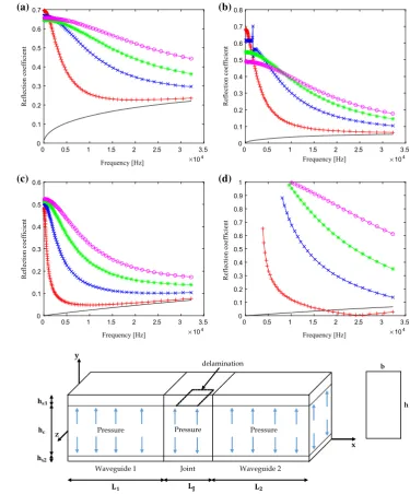
[image:13.595.186.541.56.362.2]Fig. 16 Wave reflection coefficients for the
transversely-isotropic laminate with 40% depth crack: non-pressurised (-), internal pressurep=0.1 GPa (-+), 0.5 GPa (-x), 1.0 GPa (-*) and 1.5 GPa (-o).aBending wave about y-axis.bBending wave about z-axis.cLongitudinal wave.d Torsional wave
Frequency [Hz] 104
Reflection coefficient
0 0.1 0.2 0.3 0.4 0.5 0.6 0.7
Frequency [Hz] ×
× 104
0 0.5 1 1.5 2 2.5 3 3.5 0 0.5 1 1.5 2 2.5 3 3.5
Reflection coefficient
0 0.1 0.2 0.3 0.4 0.5 0.6 0.7 0.8
Frequency [Hz] ×104
Reflection coefficient
0 0.1 0.2 0.3 0.4 0.5 0.6
Frequency [Hz] ×104
0 0.5 1 1.5 2 2.5 3 3.5 0 0.5 1 1.5 2 2.5 3 3.5
Reflection coefficient
0 0.1 0.2 0.3 0.4 0.5 0.6 0.7 0.8 0.9 1
(a) (b)
(c) (d)
Fig. 17 Schematic
representation of the WFE-FE configuration of a pressurised sandwich beam
across the surfaces of the sandwich core as shown in Fig. 17. Six different pressure scenarios are examined; one with no pressure applied and the rest with applied pressure of 0.1, 0.2, 0.3, 0.4 and 0.5 GPa per (0.001×0.002) cross sectional area.
Equation (12) is solved for the dispersion curves of the waveguide. Four propagating waves are obtained, with the remaining waves being nearfield waves. Presented in Fig. 18 are the dispersion curves of the propagating waves as a function of frequency. The curves are presented for each of the seven pressure scenarios. For the pressurised waveg-uide, a smooth, nearly linear behaviour (with regards to the wavenumbers) is observed as a function of frequency. This is observed up until a certain frequency, then a rapid rise
takes place. This behaviour is similar for all the pressure scenarios. However, the frequency at which the rapid rise is observed varies with the applied pressure. It is observed at about 1.0, 1.6, 2.2, 2.8 and 3.4 kHz respectively in the 0.1, 0.2, 0.3, 0.4 and 0.5 GPa pressurised waveguides. There is also a steady increase in the wavenumbers as a function of applied pressure. An average increase of about 27% per 0.1 GPa is observed at each frequency in the low frequency range. It should be noted that the differences are normalised as fre-quency gets higher and tend to become equal irrespective of the magnitude of pressure applied.
Fig. 18 Dispersion curves for the sandwich beam:
non-pressurised (-), pressure
p=0.01 GPa (- -), 0.1 GPa (-+), 0.2 GPa (-x), 0.3 GPa (-*), 0.4 GPa (-o) and 0.5 GPa (->). aBending wave about y-axis.b Bending wave about z-axis.c Longitudinal wave.dTorsional wave
Frequency [kHz]
102 103 104
Wavenumber [1/m]
10 20 30 40 50 60 70 80 90 100 110
Frequency [kHz]
102 103 104
Wavenumber [1/m]
10 20 30 40 50 60 70
Frequency [kHz]
102 103 104
Wavenumber [1/m]
0 1 2 3 4 5 6 7 8 9 10
Frequency [kHz]
2 103 104
Wavenumber [1/m]
0 10 20 30 40 50 60
(a) (b)
(c) (d)
40% widths delaminations in the non-pressurised sandwich beam. Due to the minute severity of the considered delami-nations, little reflection magnitudes are obtained within the considered frequency range. It can also be seen that negli-gible differences are observed between both delamination scenarios for all propagating wave types.
The reflection coefficients magnitude becomes greatly significant in the pressurised system as shown in Fig.20. Compared to the non-pressurised system, there is an aver-age change of about 50–70% in the low frequency range and of about 10–25% in the high frequency range. This can be explained by the fact that structural pre-stressing brings about change in the loss factor of the structure. In general, this consequently affects the magnitude of wave propagation properties.
As a function of frequency, the reflection magnitudes are constant over the low frequency range, then reduce slowly over the mid frequency range before reducing rapidly over the high frequency range. This behaviour is similar for all wave types and at each applied pressure.
Variation of the reflection coefficient magnitudes as a function of applied pressure is extensively examined at differ-ent frequency within each of the iddiffer-entified frequency ranges i.e., at which coefficient magnitude is constant (e.g., 0.2 kHz), slightly reduces (e.g., 0.8 kHz) and rapidly reduces (e.g., 6.4 kHz) with respect to frequency.
At 0.2 kHz (Fig.21), there is a proportional reduction of about 28% per 0.1 GPa in the reflection coefficient of the y-axis bending wave. Similar trend is observed for the z-axis bending wave. An average increment of about 30% per 0.1 GPa is observed for the torsional wave while a slight steady increment of about 2% per 0.1 GPa is observed for the longitudinal wave.
At 0.8 kHz (Fig.22), the reflection magnitudes of the x and y axes bending waves increase with the applied pressure up to 1 GPa. Beyond this pressure, reduction in the magnitudes is observed. Longitudinal and torsional waves both show simi-lar trends. There is an increase in their coefficient magnitudes with respect to applied pressure. Increment obtained for the torsional wave is however more than that of the longitudinal wave.
Frequency [kHz] ×104
5
Reflection coefficient
×10-3
0 0.2 0.4 0.6 0.8 1 1.2 1.4 1.6 1.8 2
Frequency [kHz] ×104
5
Reflection coefficient
×10-3
0 0.5 1 1.5 2 2.5 3 3.5
Frequency [kHz] ×104
0 0.5 1 1.5 2 2.5 3 3.
0 0.5 1 1.5 2 2.5 3 3.5
Reflection coefficient
×10-3
0 0.2 0.4 0.6 0.8 1 1.2 1.4
Frequency [kHz] ×104
0 0.5 1 1.5 2 2.5 3 3.
0 0.5 1 1.5 2 2.5 3 3.5
Reflection coefficient
×10-3
0 1 2 3 4 5 6
(
a
)
(b)
[image:16.595.83.513.55.432.2](c)
(
d
)
Fig. 19 Wave reflection coefficient magnitude from the 20% (-) and the 40% (- -) widths delaminations in the non-pressurised sandwich beam.a Bending wave about y-axis.bBending wave about z-axis.cLongitudinal wave.dTorsional wave
7 Concluding Remarks
This paper presents a FE-based methodology for quantify-ing wave interaction with localised structural defects. The scheme can be applied to structures of arbitrary complex-ity, layering and material characteristics as FE discretisation is employed. The scheme discretises defective structural waveguide into a system of two pristine waveguides con-nected through a defective coupling joint. The wave propa-gation properties within the pristine waveguides are coupled to the localised defect in the joint in order to compute the wave reflection and transmission properties for each propa-gating wave mode in the system. The presented methodology also examine the effect of pre-stress on the wave propaga-tion and transmission properties of pressurised structures. The principal outcome of the work can be summarised as follows:
(a) The presented approach is validated with analytical and full FE transient response predictions. Very good agree-ment is observed.
(b) The approach is able to predict the dispersion properties of an arbitrarily complex structure as well as the reflec-tion and transmission coefficients of the wave interacreflec-tion with defects within the structure.
(c) The approach also successfully examined the effect of pre-stress on the wave properties of pressurised struc-tures. It was shown that pressurisation can be used to detect micro defects which may be too small to detect under no pressurisation.
Fig. 20 Wave reflection coefficient magnitude from the 20% (-) width delamination within the sandwich beam: non-pressurised (-), pressure
p=0.01 GPa (- -), 0.1 GPa (-+), 0.2 GPa (-x), 0.3 GPa (-*), 0.4 GPa (-o) and 0.5 GPa (->). aBending wave about y-axis.b Bending wave about z-axis.c Longitudinal wave.dTorsional wave
Frequency [kHz]
102 103 104
Reflection coefficient
0 0.1 0.2 0.3 0.4 0.5 0.6 0.7
Frequency [kHz]
102 103 104
Reflection coefficient
0 0.1 0.2 0.3 0.4 0.5 0.6
Frequency [kHz]
102 103 104
Reflection coefficient
0 0.05 0.1 0.15 0.2 0.25 0.3 0.35 0.4 0.45 0.5
Frequency [kHz]
102 103 104
Reflection coefficient
0 0.1 0.2 0.3 0.4 0.5 0.6 0.7 0.8
(a) (b)
(c) (d)
Fig. 21 Wave reflection coefficient magnitude at 0.2 kHz for the pressurised sandwich beam as a function of applied pressure: 20% (-) width delamination, 40% (- -) width delamination.aBending wave about y-axis.bBending wave about z-axis.cLongitudinal wave.dTorsional wave
Applied pressure [GPa]
5
Reflection coefficient
0.58 0.6 0.62 0.64 0.66 0.68 0.7
Applied pressure [GPa]
5
Reflection coefficient
0.48 0.5 0.52 0.54 0.56 0.58 0.6 0.62 0.64 0.66
Applied pressure [GPa]
5
Reflection coefficient
0.15 0.2 0.25 0.3 0.35 0.4 0.45 0.5
Applied pressure [GPa]
0 0.1 0.2 0.3 0.4 0. 0 0.1 0.2 0.3 0.4 0.
0 0.1 0.2 0.3 0.4 0. 0 0.1 0.2 0.3 0.4 0.5
Reflection coefficient
0.1 0.2 0.3 0.4 0.5 0.6 0.7 0.8
(a) (b)
Fig. 22 Wave reflection coefficient magnitude at 0.8 kHz for the pressurised sandwich beam as a function of applied pressure: 20% (-) width delamination, 40% (- -) width delamination.aBending wave about y-axis.bBending wave about z-axis.cLongitudinal wave.dTorsional wave
Applied pressure [GPa]
5
Reflection coefficient
0.5 0.52 0.54 0.56 0.58 0.6 0.62 0.64 0.66 0.68
Applied pressure [GPa]
5
Reflection coefficient
0.42 0.44 0.46 0.48 0.5 0.52 0.54 0.56 0.58 0.6
Applied pressure [GPa]
0 0.1 0.2 0.3 0.4 0.
0 0.1 0.2 0.3 0.4 0.5
Reflection coefficient
0 0.05 0.1 0.15 0.2 0.25 0.3 0.35 0.4 0.45 0.5
Applied pressure [GPa]
0 0.1 0.2 0.3 0.4 0.
0 0.1 0.2 0.3 0.4 0.5
Reflection coefficient
0 0.1 0.2 0.3 0.4 0.5 0.6 0.7 0.8
(a) (b)
(c) (d)
Fig. 23 Wave reflection coefficient magnitude at 6.4 kHz for the pressurised sandwich beam as a function of applied pressure: 20% (-) width delamination, 40% (- -) width delamination.aBending wave about y-axis.bBending wave about z-axis.cLongitudinal wave.dTorsional wave
Applied pressure [GPa]
5
Reflection coefficient
0 0.1 0.2 0.3 0.4 0.5 0.6
Applied pressure [GPa]
5
Reflection coefficient
0 0.05 0.1 0.15 0.2 0.25 0.3 0.35 0.4 0.45
Applied pressure [GPa]
0 0.1 0.2 0.3 0.4 0.
0 0.1 0.2 0.3 0.4 0.5
Reflection coefficient
-0.05 0 0.05 0.1 0.15 0.2 0.25 0.3 0.35
Applied pressure [GPa]
0 0.1 0.2 0.3 0.4 0.
0 0.1 0.2 0.3 0.4 0.5
Reflection coefficient
0 0.1 0.2 0.3 0.4 0.5 0.6 0.7
(a) (b)
Open Access This article is distributed under the terms of the Creative Commons Attribution 4.0 International License (http://creativecomm ons.org/licenses/by/4.0/), which permits unrestricted use, distribution, and reproduction in any medium, provided you give appropriate credit to the original author(s) and the source, provide a link to the Creative Commons license, and indicate if changes were made.
References
1. Heslehurst, R.: Defects and Damage in Composite Materials and Structures. CRC Press, Boca Raton (2014)
2. Kessler, S., Spearing, S., Soutis, C.: Damage detection in composite materials using lamb wave methods. Smart Mater. Struct.11, 269– 278 (2002)
3. Raju, P.: Acousto-ultrasonic technique for nondestructive evalua-tion of composites and structures. Acoust. Soc. Am. J.102, 3082 (1997)
4. Chien, H., Sheen, S., Raptis, A.: An acousto-ultrasonic nde tech-nique for monitoring material anisotropy. In: Thompson, D.O., Chimenti, D.E. (eds.) Review of Progress in Quantitative Nonde-structive Evaluation, pp. 1225–1232. Springer, New York (1993) 5. Worlton, D.: Ultrasonic testing with lamb waves. Non-Destr. Test.
15, 218–222 (1957)
6. Rose, J.: Ultrasonic Waves in Solid Media. Cambridge University Press, Cambridge (2004)
7. Donskoy, D., Sutin, A.: Vibro-acoustic modulation nondestruc-tive evaluation technique. J. Intell. Mater. Syst. Struct.9, 765–771 (1998)
8. Su, Z., Zhou, C., Hong, M., Cheng, L., Wang, Q., Qing, X.: Acousto-ultrasonic based fatigue damage characterization: linear versus nonlinear signal features. Mech. Syst. Signal Process.45, 225–239 (2014)
9. Lowe, M.: Matrix techniques for modelling ultrasonic waves in multi-layered media. IEEE Trans. Ultrason. Ferroelectr. Freq. Cont. 42, 525–542 (1995)
10. Young, Y., Lin, Y.: Dynamic response analysis of truss-type struc-tural networks: a wave propagation approach. J. Sound Vib.155, 375–381 (1992)
11. Hutchinson, R., Fleck, N.: The structural performance of the peri-odic truss. J. Mech. Phys. Solids54, 756–782 (2006)
12. Mace, B.: Wave reflection and transmission in beams. J. Sounds Vib.72, 237–246 (1984)
13. Chouvion, B., Popov, A., McWilliam, S., Fox, C.: Vibration modelling of complex waveguide structures. Comput. Struct.89, 1253–1263 (2011)
14. Yuana, W., Zhoua, L., Yuanb, F.: Wave reflection and transmis-sion in composite beams containing semi-infinite delamination. J. Sounds Vib.313, 676–695 (2007)
15. Doyle, J.: Wave Propagation in Structures: Spectral Analysis Using Fast Discrete Fourier Transforms. Springer, New York (1997) 16. Hosten, B., Castaings, M.: Finite elements methods for modeling
the guided waves propagation in structures with weak interfaces. J. Acoust. Soc. Am.117, 1108–1113 (2005)
17. Pialucha, T., Cawley, P.: The reflection of ultrasound from interface layers in adhesive joints. Review of Progress in Quantitative Non-destructive Evaluation, pp. 1303–1309. Springer, Boston (1991) 18. Leung, R., Pinnington, R.: Wave propagation through right-angled
joints with compliance: longitudinal incidence wave. J. Sound Vib. 153, 223–237 (1992)
19. Nayfeh, A.H., Chimenti, D.E.: Ultrasonic wave reflection from liquid-coupled orthotropic plates with application to fibrous com-posites. J. Appl. Mech.55, 863–870 (1988)
20. Zienkiewicz, O.C., Taylor, R.L.: The Finite Element Method: Solid Mechanics, vol. 2. Butterworth-heinemann, Oxford (2000)
21. Mead, D.: A general theory of harmonic wave propagation in linear periodic systems with multiple coupling. J. Sounds Vib.27, 235– 260 (1973)
22. Langley, R.: A note on the force boundary conditions for two-dimensional periodic structures with corner freedoms. J. Sounds Vib.167, 377–381 (1993)
23. Mace, B.R., Duhamel, D., Brennan, M.J., Hinke, L.: Finite element prediction of wave motion in structural waveguides. J. Acoust. Soc. Am.117(5), 2835–2843 (2005)
24. Waki, Y., Mace, B., Brennan, M.: Numerical issues concerning the wave and finite element method for free and forced vibration of waveguides. J. Sounds Vib.327(1–2), 92–108 (2009)
25. Mencik, J.-M., Ichchou, M.: Multi-mode propagation and diffusion in structures through finite elements. Eur. J. Mech. A24(5), 877– 898 (2005)
26. Chronopoulos, D., Troclet, B., Bareille, O., Ichchou, M.: Modeling the response of composite panels by a dynamic stiffness approach. Compos. Struct.96, 111–120 (2013)
27. Manconi, E., Mace, B.: Modelling wave propagation in two-dimensional structures using a wave/finite element technique. ISVR Technical Memorandum, (2007)
28. Chronopoulos, D., Troclet, B., Ichchou, M., Laine, J.: A unified approach for the broadband vibroacoustic response of composite shells. Compos. B43(4), 1837–1846 (2012)
29. Apalowo, R., Chronopoulos, D., Ichchou, M., Essa, Y., Martin De La Escalera, F.: The impact of temperature on wave interaction with damage in composite structures. Proc. Inst. Mech. Eng. C231(16), 3042–3056 (2017)
30. Apalowo, R., Ampatzidis, T., Chronopoulos, D., Ichchou, M., Essa, Y., De La Escalera, F.: Prediction of temperature dependent wave dispersion and interaction properties in composite structures. In: Proceedings of the 24th International Congress on Sound and Vibration, 23–27 July 2017, London, (2017)
31. Chronopoulos, D., Droz, C., Apalowo, R., Ichchou, M., Yan, W.: Accurate structural identification for layered composite structures, through a wave and finite element scheme. Compos. Struct.182, 566–578 (2017)
32. Renno, J.M., Mace, B.R.: Calculation of reflection and transmis-sion coefficients of joints using a hybrid finite element/wave and finite element approach. J. Sound Vib.332(9), 2149–2164 (2013) 33. Cook, R.: Concepts and Applications of Finite Element Analysis,
2nd edn. Wiley, New York (1981) 34. ANSYS, ANSYS 14.0 User’s Help, (2014)
35. Talreja, R., Singh, C.: Damage and Failure of Composite Materials, Damage and Failure of Composite Materials. Cambridge Univer-sity Press, Cambridge (2012)
36. Nag, A., Mahapatra, D., Gopalakrishnan, S., Sankar, T.: A spec-tral finite element with embedded delamination for modeling of wave scattering in composite beams. Compos. Sci. Technol.63(15), 2187–2200 (2003)
37. Petyt, M.: Introduction to Finite Element Vibration Analysis. Cam-bridge University Press, CamCam-bridge (2010)
38. Cremer, L., Heckel, M., Petersson, B.: Structure Borne Sound: Structural Vibrations and Sound Radiation at Audio Frequencies. Springer, New York (2005)


![Fig. 12 Comparison of the wave reflection coefficients from notch ofdepth.varying depths: Presented WFE-FE methodology (-), Full FE predic-tions (- -) and Experimental measurements (◦) in [39]](https://thumb-us.123doks.com/thumbv2/123dok_us/8552670.363298/11.595.309.541.56.472/comparison-reection-coefcients-ofdepth-presented-methodology-experimental-measurements.webp)