A Nonlinear Analytical Model for the
Rapid Prediction of the Torque of
Synchronous Reluctance Machines
Giacomo Bacco,
Student Member, IEEE,
Nicola Bianchi,
Fellow, IEEE,
Hanafy Mahmoud
Abstract—The synchronous reluctance motor works under
heavy saturation. This paper presents a nonlinear analytical model of the reluctance machine, which is used to derive both average and torque harmonics as a function of the rotor geometry. Maps showing the torque harmonics as a function of the rotor barrier angles are derived. These maps are useful tools for the machine designer to get a proper rotor geometry. The torque maps are compared with those obtained from both linear analytical and finite element models. The maps computed analytically show good agreement with those derived by means of finite element analysis, and they are obtained in a much smaller computing time.
Index Terms—Electric machines, AC motors, Design tools, Synchronous reluctance machine, Analytical model, Saturation
I. INTRODUCTION
B
OTH synchronous reluctance (REL) and permanent mag-net assisted reluctance (PMAREL) machines are more and more used, ranging from low- to medium-power applications as alternatives to the more expensive rare-earth magnet motors and to the less efficient induction motors [1]–[3]. Although the intrinsic advantages of these machines, a thoughtful design is key to reach the goals of good performance and high efficiency [4]–[6]. In particular, one of the most important design step is the choice of the number of flux-barriers and their end-angles [7], [8].At first, the model with linear B-H characteristic is de-scribed. Then the model is extended to include the saturation of some parts of the machine. Conversely to previous models, the saturation is taken into account following all the main flux lines paths inside the machine. Then a proper saturation coefficient is assigned to each of this path and applied at the air-gap. The analytical model proves to be fast and fairly accurate in any calculation. Therefore it is quick and easy to obtain the behavior of the average torque and torque ripple as a function of the rotor flux-barrier geometry. The result is presented using maps, which are essential for finding a proper combination of barrier angles which gives maximum average torque and minimum torque ripple.
Manuscript received October 12, 2017; revised January 10, 2018; ac-cepted February 4, 2018. Paper no. TEC-00790-2017. (Corresponding au-thor: Giacomo Bacco.) Giacomo Bacco and Nicola Bianchi are with the Electrical Drives Laboratory, Department of Industrial Engineering, Univer-sity of Padova, Padova, 35131, Italy (e-mail: [email protected]; [email protected]). Hanafy Mahmoud is with the Department of Electri-cal and Electronic Engineering, University of Nottingham, NG72RD, Notting-ham (UK), and also with the Department of Electrical Power and Machines, Cairo University, 12613 Giza, Egypt (e-mail: [email protected]).
–A
+A
d-axis
a-axis
+A
[image:1.612.316.565.203.399.2]–A
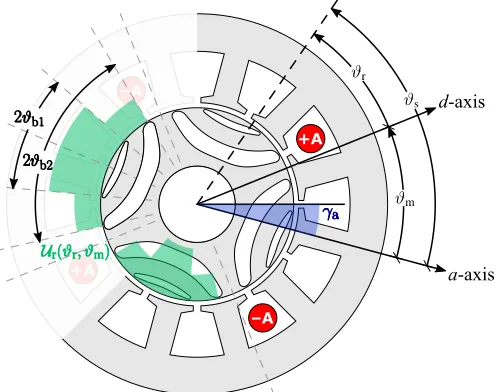
Fig. 1: Sketch of a RELmotor with two flux-barriers per pole together with the reference axes and the barrier angle quotes. The colored area on top of the flux-barriers represents the rotor magnetic scalar potential distribution for half the machine.
II. ANALYTICAL MODEL
The analytical model considersRELmachines with transver-sally laminated rotor. Furthermore, only integral-slot winding are considered. The electric loading of a symmetric three-phase distributed winding is [8]:
Ks(ϑs, ϑm) =
∞ X
ν=6k+1 k∈Z
ˆ
Kνsin νpϑs−pϑm−αei
(1)
whereν is the space harmonic order whose values belong to the set {1,−5,7,−11,13, . . .}, Kˆν is the amplitude of the electric loadingν-th harmonic,pis the number of pole pairs,
ϑsis the angular coordinate fixed to the stator,ϑm is the rotor angular position, andαe
iis the current electric angle. It is worth noticing that (1) reproduces every space harmonic generated by the discretized winding.
The electric loading gives rise to the stator magnetic scalar potential, given by
Us(ϑs, ϑm) =
Z
Ks(ϑs, ϑm)
D
whereDis the stator diameter at the air-gap. For a three-phase machine it is
Us(ϑs, ϑm) =−
D 2
X
ν=6k+1 k∈Z
ˆ Kν
pν cos(νpϑs−pϑm−α
e i) (3)
Similarly, the rotor magnetic scalar potential, which reacts to the stator potential, can also be expressed by means of its Fourier series expansion
Ur(ϑr, t) =
+∞ X
ξ=1 ˆ
Uξsin(ξpϑr) (4)
It is different from zero when the flux flows in the q-axis direction, crossing the flux-barriers. The rotor magnetic scalar potentials and the rotor barrier angles are grouped in vectors:
ur={Ur1, Ur2, . . . , Urn}T, (5)
ϑb={ϑb1, ϑb2, . . . , ϑbn}T (6) A quasi-diagonal matrix Gcan be built, given by
G=
+1 −1
[image:2.612.306.558.53.295.2]+1 −1
. .. ...
+1 −1
+1
(7)
with+1in the main diagonal and−1in the second right-hand diagonal, such that
ˆ Uξ=
4 πξsin ξ
π
2 sin(ξpϑ
T b)Gur
(8) wheresin(ξϑT
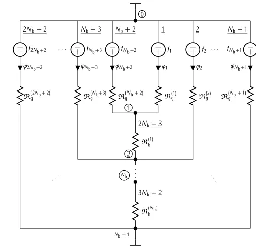
b)is a row vector of sines,Gur is the product of the matrix (7) and the vectorur, defined in (5). The magnetic potentials of the islands can be calculated as the solution of the magnetic circuit shown in Fig. 2. The stator magnetic scalar potential, given in (3), can be expressed in the rotor reference frame. Since
ϑs=ϑr+ϑm (9)
it results in
Us(ϑr, ϑm) =−
X
ν=6k+1 k∈Z
ˆ KνD
2pν cos
νpϑr+ (ν−1)pϑm−αei
(10) It is split using sine and cosine as:
Us(ϑr, ϑm) =−
X
ν=6k+1
k∈Z
ˆ
KνD
2pν
h
cos(νpϑr) cos (ν−1)pϑm−αei
+
−sin(νpϑr) sin (ν−1)pϑm−αei
i
(11)
Ur(ϑr, ϑm) also contains harmonics multiple of three and they can be grouped apart. Then, it is easy to verify that Ur is an even function with respect to the harmonic order ξ, so positive or negative indexes can be used indifferently.
Ur(ϑr, ϑm) =
X
ν=6k+1 k∈Z
ˆ
Uνsin(νpϑr) +
X
µ=6h+3 h∈Z+
ˆ
Uµsin(µpϑr)
(12)
0
1
+
− f1
φ1
R(1)g
Nb+ 2
+
− fNb +2
φNb +2
R(Nb + 2)
g
2
+
− f2
φ2
R(2)g
Nb+ 3
+
− fNb +3
φNb +3
R(Nb+3) g
Nb+ 1
+
−
fNb +1
φNb +1
R(Nb + 1)
g
2Nb+ 2
+
− f2Nb +2
φ2Nb +2
R(2Nb + 2)
g
1
2Nb+ 3
R(1) b
2
. . .
Nb
3Nb+ 2
R(Nb ) b
Nb + 1
· · · · · ·
. ..
. ..
Fig. 2: Magnetic circuit of one pole of the rotor of a REL machine. Circled labels represent nodes while underlined labels represent edges of the circuit.
The air-gap flux density can be expressed as the difference of the two magnetic scalar potentials [8], [9]:
Bg(ϑr, ϑm) =µ0
−Us(ϑr, ϑm) +Ur(ϑr, ϑm)
g (13)
Introducing (11) and (12) in (13), the air-gap flux density results in
Bg=
X
ν=6k+1 k∈Z
µ0DKˆν
2gp ν
z stator even part}| { cos (ν−1)ωt−αe
i
cos(νpϑr)
−sin (ν−1)ωt−αe
i) sin(νpϑr)
| {z }
stator odd part
+
+ X
ν=6k+1 k∈Z
µ0
gννUˆνsin(νpϑr)
| {z }
rotor without triplen harmonics
+ X
µ=6h+3 h∈Z+
µ0
gµµUˆµsin(µpϑr)
| {z }
rotor triplen harmonics and reordering
Bg(ϑr, ϑm) =
X
ν
αν
ν cos(νpϑr) + βν
ν sin(νpϑr)
+
+X
µ
γµ
µ sin(µpϑr)
(14)
whereαν, βν derives from the coefficients which multiply the cosine and sine functions under the summations in ν, while
γµ=µ0µUˆµ/g.
0 50 100 150
−2 −1 0 1 2
Rotor coordinate, ϑ
r (deg)
Air−gap flux density, B
g
(T) B
g Us
U r
0 50 100 150 −1000
−500 0 500 1000
[image:3.612.313.562.54.232.2]Magnetic scalar potential (A)
Fig. 3: Air-gap flux density and magnetic scalar potentials of a 2-barrier REL machine without saturation att= 0.
A. Torque derivation
The torque is obtained integrating the Lorentz’s force den-sity KsBg, both function of ϑr and ϑm (omitted hereafter), along the air-gap surface and multiplying the result by the lever-arm D/2 [8]:
τm(ϑm) =−
D 2
Z 2π
0
BgKs
DLstk
2 dϑr (15)
Remembering (13), it can be derived
τm=
µ0D2Lstk
4g
Z 2π
0
UsKsdϑr
| {z }
A
−
Z 2π
0
UrKsdϑr
| {z }
B
(16)
The first integral, labeled as A, is zero since Us andKs are orthogonal functions. Therefore the torque is only due to the interaction of electric loading Ks and the magnetic scalar potential of the rotorUr.
The final expression of the torque is
τm(ϑm) =−
µ0D2Lstk
g
X
ν,k
ˆ Kν
ν sinν
π 2·
·cos (ν−1)pϑm−αei
sin(νϑT)Gur
(17)
B. Tooth flux density
To compute the stator tooth flux density, the air-gap flux density Bg(ϑr, ϑm) in (14) has to be referred to the stator reference frame. It is
Bg(ϑs, ϑm) =X
ν
αν
ν cos(νpϑs−νpϑm) + βν
ν sin(νpϑs−νpϑm)
+X
µ
γµ
µ sin(µpϑs−µpϑm) (18)
The stator tooth flux density can be obtained through the scaled average of the air-gap flux density [10]–[12]:
Bt(ϑm) =
ps
αswtkpack
Z ϑd+αs ϑd
Bg(ϑs, ϑm)dϑs (19)
wherepsis the slot pitch,αsthe slot angle,wtthe tooth width, and kpack is the ratio between the total effective iron and the stack length.
It can be demonstrated that the tooth flux density assumes
q different behaviors, q being the number of slots per pole
channel
1st island
Nbth island
1
Nb ...
...
[image:3.612.54.298.62.188.2]... ...
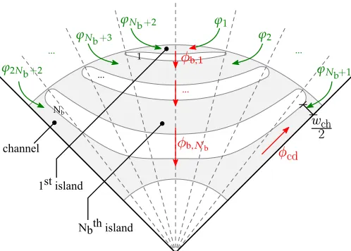
Fig. 4: Sketch of the main parts of the rotor structure and rotor fluxes direction.
and per phase, defined asq=Q/(m2p). Thus the integration extremes can be expressed as
ϑd= (d−1)αs−γa, d= 1, . . . , q (20) whereγa identifies the angular position of the magnetic axis of phaseawith respect to the first slot (see Fig. 1).
C. Stator yoke flux density
The flux in the stator yoke—also referred to as back-iron— is obtained integrating the air-gap flux density over a pole pitch, then the flux density is
By(ϑm) =
1 2hykpack
Z πp−γa
−γa
Bg(ϑs, ϑm)
D 2 dϑs
= ↑ qinteger
wt
2hy Q/2p
X
i=1
Bt,i(ϑm) (21)
wherehy= (De−D)/2is the stator yoke height.
D. Rotor fluxes
In the linear case, the fluxes entering the rotor are directly obtained from the solution of the magnetic circuit in Fig 2. Both the island and the barrier fluxes are computed. The iron path closer to the shaft is referred to as channel. The remaining iron paths for thed-axis flux are referred to as islands. They assume a different potential, due to the q-axis flux, and they are numbered accordingly to the number of the barrier beneath them. The barrier fluxes are obtained solving the magnetic network depicted in Fig. 2. The d-axis channel flux comes from φcd = ϕNb+1 −ϕ2Nb+2 which simply sums the two
fluxes to obtain the whole direct flux of the channel. Then
Bcd=
φcd
wchkpackLstk
(22) wherewch≈(1−kair)Dsin 2πp−ϑbNb
For the q-axis flux of the main channel, just half of the last barrier flux can be considered, with φcq=φb,Nb/2. Thus
Bcq=
φcq
lchkpackLstk
(23) wherelch= (Dre−Dri)/2. Then, it is
|Bc|=
q B2
cd+B2cq (24)
The d-axis fluxes of the islands result directly from the magnetic circuit fluxes, as
Bid,j =
ϕj
kpackLstkwisl,j
(25) Regarding theq-axis fluxes of the islands, the average of the fluxes above and beneath each island is computed. An average cross-section area of each island is considered, so that
ϑisl,j= ϑb, j+ϑb, j−1
2 (26)
lisl,j=ϑisl,jD (27)
φiq,1 φiq,2 φiq,3
.. .
φiq,Nb
= 1 2
2 1 1
1 1
. .. ...
1 1
φb1 φb2 φb3
.. .
φbNb
(28)
Biq,j=
φiq,j
kpackLstklisl,j
(29)
|Bi,j|= q
B2
id,j+B2iq,j (30)
III. ANALYTICAL MODEL WITH SATURATION The previous analytical model works properly in case of linear behaviour of ferromagnetic material, that is, in the first part of the ironB-H curve. However, this condition is barely met. InRELmotors the rotor iron paths are saturated to achieve a quite high torque density and power factor. Thus, in practice, the saturation of the machine has to be taken into account.
Hereafter, the saturation is taken into account through a discretization of the flux line paths into sections. In particular, a section can be a stator tooth, a stator yoke sector, or a rotor half iron path. The path of a flux line results a succession of these sections. Therefore a magnetic voltage drop and a saturation factor are associated with each flux line and referred to the air-gap. At first the rotor iron paths are considered, and then the stator teeth and yoke.
A. Rotor channel and islands magnetic voltage drop
The magnetic voltage drop of the rotor channel is estimated from (24). Since the flux density is computed in the smallest cross-section, it is the maximum value of the channel. The average is estimated asB⋆
c = 0.85|Bc|and, from the ironB
-H curve, the magnetic fieldHcis obtained (in the following, it is indicated as B → H). Then the magnetic voltage drop results ψc = Hclch. Similarly, the islands have a complex geometry and a different flux density in every point. The
middle section of the island is considered, where the width is precisely known. It should be noted that the two half-island paths have different voltage drops due to part of the entering elementary flux that crosses the barrier and does not reclose on the other side. To recover this difference, a magnetic voltage drop is computed for every half island using the elementary flux.The procedure is sketched as follows:
|Bi,j| −→ Hi,j then ψi,j =Hi,jlisl,j
2 (31)
The same procedure is carried out for the second (South) half pole.
The vector of rotor magnetic voltage drops, corresponding to the sequence of channel and islands starting from the origin of ϑr, is:
ψrp={ψc, ψi,Nb, . . . , ψi,1
| {z }
ψN
i
ψi,Nb+ 2, . . . , ψi,2Nb+ 2
| {z }
ψSi
, ψc}T
where ψN
i and ψ S
i are the vectors of the first half pole (identified by the superscript N meaning North) and the second half pole (identified by the superscript S meaning South) voltage drops, respectively.
Numerically, this vector is distributed into a number of points accordingly to the angle spanned. In the end, the distribution of the rotor magnetic voltage drops is equivalent to the distribution of the scalar magnetic potentials along the air-gap.
ψr =
ψc, . . . , ψc
| {z }
N Nb+ 1
, ψi,Nb, . . . , ψi,Nb
| {z }
N Nb
, . . . , ψi,1, . . . , ψi,1
| {z }
N1
, . . .
| {z }
Res/2p
T
whereRes is the number of points used for discretizing the
space[0,2π] along the air-gap, and the subscript of N refers to the corresponding island.
B. Stator teeth and yoke magnetic voltage drops
The instantaneous tooth flux density in the saturation case is obtained through the numerical integration of (19). Once the flux density for every tooth of interest (typicallyQ/pteeth for an integer-slot winding) is computed, the magnetic voltage drops are derived, as follows:
|Bt, j| −→ Ht,j then ψt,j=Ht,jhs (32)
wherehs is the tooth height.
The back-iron corresponding to a pole pair is split intoQ/p
parts, each one covering a slot angle, as illustrated in Fig. 5 (dotted lines). The flux density can be derived for each part, as
˜
φy(k) =wtLstk k X
j=1
Bt, j k= 1, . . . , Q/p (33)
φy(k) = ˜φy(k)−
1 Q/p
Q/p X
j=1 ˜
φy(j) (34)
By(k) =
|φy(k)|
hyLstk
∆ly ψy
ψy(1)
ψy(2)
ψy(9)
ψy(5)
path 5-14
[image:5.612.52.301.55.209.2]path 1-10 (13)
Fig. 5: Real flux lines and main integration paths (Q = 36,2p= 4).
where∆l=π(De−hy)/Qis the average length of one back-iron part. Once the stator yoke voltage drops are computed in any section, the flux path for all flux lines of interest have to be correctly identified. Two of these lines are shown in Fig. 5. Summing the voltage drops along these lines is equivalent to consider that each flux line flows for a full pole and it encounters Q/2p voltage drops along its path. The voltage drops are summed with the sign of the corresponding flux in the same part. Finally, every flux line has gathered the same overall magnetic voltage drop of the actual flux line of that particular tooth. Therefore, it is
ψyt(n) =
1 2
n+Q
2p−1 X
k=n
ψy(k) signφy(k)
, n= 1, . . . , Q/2p (36)
where the double subscript ‘yt’ indicates that the yoke drop is referred to the tooth. The 12 occurs since half the path is counted. For example, let us consider the path 1-10 shown in Fig. 5, which covers ψy(1) to ψy(9): it starts from tooth number 1 (below the first slot) and it ends in tooth 10. The total magnetic voltage drop associated to this line is
2ψyt(1) =ψy(1) +ψy(2) +. . .+ψy(9) (37) On the other hand, along the path5-14it is
2ψyt(5) =ψy(5) +. . .+ψy(9)−ψy(10)−. . .−ψy(13)
∼
=ψy(5) (38)
The last equivalence is the main assumption of this compu-tation. In fact it implies that ψy(6) is equal to ψy(13) and so on, and the remaining term is just ψy(5). Even if the machine is not symmetrically magnetized, this is a fairly good approximation thanks to the lower value of theq-axis flux with respect to thed-axis flux. Even with high values of αe
i it can be shown that this approximation is good enough.
Similarly to the rotor, the stator magnetic voltage drops can be collected and distributed along the discretization of the angular coordinate at the air-gap.
C. Total magnetic voltage drop and saturation factor
In order to combine the rotor and stator magnetic voltage drop distributions, the rotor position and the first tooth dis-placement have to be taken into account through the shift of one of the two distributions, according to the adopted reference frame. The air-gap magnetic voltage drop can be easily computed from the flux density obtained in the previous iteration.
Ψg=Hgg= Bg
µ0
g (39)
All the magnetic voltage drops are summed to obtain the total voltage drop, which is again referred to the air-gap.
Ψtot=Ψg+Ψrs+Ψr (40)
where Ψr
s is the vector of stator voltage drops in the rotor reference frame. Then
ksat=
Ψtot
Ψg (41)
This saturation factor is different from the usually adopted factor. In fact (41) is a distribution of saturation factors along the air-gap that better represents the saturation of the machine. The adopted iteration scheme is fixed-point like, with a random relaxation to improve the stability of the convergence:
k(satm+ 1)←k
(m)
sat + 0.5rand
k(satm+ 1)−k
(m)
sat
(42) For the next iteration the updated air-gap flux density is simply
B(gm+ 1)=µ0
−Us+Ur
k(satm+ 1)g
(43) and the iteration cycle restarts. The error of the method was evaluated through
ǫsat=
k
(m+ 1)
sat −k
(m)
sat
(44)
IV. TORQUE MAPS
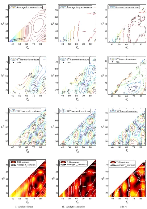
The nonlinear model is used to compute the impact of the rotor geometry on both the average torque and torque ripple. In particular, the impact of the flux-barrier-end angles is analyzed, since they heavily affect the torque ripple [8]. The average torque and some torque ripple harmonics are computed as a function of the flux-barrier angles, ϑb1, ϑb2,
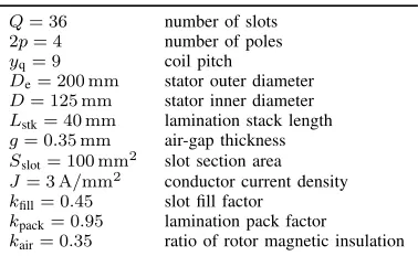
[image:5.612.344.533.629.745.2]and their amplitude is shown graphically by using maps. Fig. 6 reports such torque maps, computed for a reference motor with two flux barriers whose data is reported in Table I:
TABLE I: Parameters of the reference motor.
Q= 36 number of slots 2p= 4 number of poles
yq= 9 coil pitch
De= 200 mm stator outer diameter
D= 125 mm stator inner diameter
Lstk= 40 mm lamination stack length
g= 0.35 mm air-gap thickness
Sslot= 100 mm2 slot section area
J= 3 A/mm2 conductor current density
kfill= 0.45 slot fill factor
kpack= 0.95 lamination pack factor
For the sake of an easy comparison, Fig. 6 reports three
columns, which refer to the results obtained by means of:
i. the analytical linear model [8], ii. the nonlinear model, described above,
iii. the FE method applied on the same motor geometries [13]–[15].
The results on synchronousRELmotor achieved throughFE analysis have been compared with experimental test several times by the authors, obtaining satisfactory agreements [8], [16]–[18] but also in other works [19]–[21]. For this reason, in the following comparison, the results computed analytically are considered to be valid if they agree with the FEresults.
Thefirst rowreports the comparison among average torque
maps. The map computed with the linear model shows higher average torques with respect to the other two maps. This is obvious since the model does not take into account the iron saturation. However, it is worth noticing that the behavior of the torque curves is almost identical.
Comparing the maps of the second and third column, it is possible to note that the nonlinear analytical model predicts correctly not only the behavior of the torque maps as a function ofϑb1andϑb2, but also its amplitude. Therefore, the nonlinear
model can be used as an alternative toFEsimulation to derive such a map.
For this machine configuration, the average torque is almost independent of the first barrier angle. It can be noted that the average torque reaches its maximum in a wide region. For instance, for ϑe
b2 > 60◦ the maps are quite flat. Thus the
designer is free to move within this space looking for torque ripple minima. This behaviour is reflected also by theFEmap.
The second row shows the maps of the torque harmonic
of order 6, which is the lowest order one. Independently from the model used, it appears that there is an evident minimum—highlighted by the black dot—corresponding to the angle combination(ϑe
b1, ϑeb2) = (36◦,72◦). Such a point is
coincident in the maps obtained from the linear and nonlinear analytical models, while it is a bit shifted whenFEis used. This is caused by the local saturation of tooth tips and iron parts, which is not considered in the analytical models. In addition, it can be noted that the torque ripple contours obtained by the three models are in a satisfactory agreement in the whole region.
The same considerations can be made comparing the maps for thethird row, which report the torque harmonic of order 18. Such a torque harmonic corresponds to the first magnetic scalar potential (also referred to as MMF) slot harmonic. They are the MMF harmonics produced by the winding discretized inside the slots (18 = 36 slots/2 pole pairs), which are characterized by a winding factor equal to the fundamental one. They typically cause the highest ripple. It can be noted that the number of peaks and valleys is increased with respect to the sixth torque harmonic. This trend is general: the higher the harmonic order, the higher the number of maxima and minima. Once more, peaks and valleys predicted by the linear analytical model and nonlinear analytical models are in a good agreement with those found by FE.
Finally, in thelast row the maps compare the torque total harmonic distortion (THD), defined as
THD=
qP h6=0τˆh2
τ0
(45) where τ0 is the average torque. The filled map shows THD
contours, while the white superimposed contours refer to the average torque map. The brighter the color, the higher the THD. Thus, as far as the torque ripple is concerned, the better combinations of (ϑe
b1, ϑeb2) are those corresponding to the
darker areas.
Furthermore, by comparing the results of the third and fourth rows, it can be observed that bright colors correspond to the peaks of torque harmonic of 18th order, which is due to the MMF slot harmonics. This highlights the heavy impact of the MMF slot harmonics on the overall torque ripple.
Finally, as an overall conclusion, the linear and nonlinear analytical models produce a behavior of average torque map very similar to that obtained through FE, with the difference that the linear map has higher values than the other two models. Therefore, the nonlinear analytical model has to be adopted to predict the average torque. On the other hand, both the analytical models are able to find the position of maxima and minima of the torqueTHD. Thus, it can be stated that even the linear model can be used in spite of the nonlinear one when searching for the flux-barrier angle combinations exhibiting a minimum torque ripple, with the advantage of a higher speed and similar accuracy. The slight shifts of maxima and minima found by the FE maps are mainly due to the local saturation of iron, which is not taken into account in the linear analytical model.
V. CONCLUSIONS
This paper has shown an accurate nonlinear analytical model for the synchronous reluctance machine. A good agreement between analytical andFEsimulations has been achieved, even in highly saturated machines.
Thanks to the speed of the analytical model, it is possible to quickly obtain some maps of torque harmonics as a function of the barrier-end angles. These maps can be a useful design tool for the design of a reluctance machine. Overall, the analytical maps are able to properly estimate the FEmaps.
The average torque behavior is correctly predicted by the nonlinear analytical model, while the linear model overesti-mates it. However, even if there are some differences in the amplitude prediction, the angle combinations corresponding to the minima and maxima are correctly estimated, by means of both the linear and nonlinear models. This fact is quite significant because it suggests that the analytical linear model can be employed to get good design points in the barrier-angle plane for a specific motor in a small amount of time (some minutes). On the other hand, the nonlinear analytical model is used to properly predict the average torque.
REFERENCES
5.6 5.7 5.8 5.9 66.1 6.2 6.3 6.4 6.5 6.6 6.7 6.8 6.8 6.9 6.9 6.9 7 7 7 7 7 7.1 7.1 7.1 7.1 θ b2 e θ b1 e
40 50 60 70 80
30 40 50 60 70
Average torque contours
3.6 3.8 4 4.2 4.4 4.6 4.6 4.8 4.8 4.8 4.8 4.8 5 θ b2 e θ b1 e
40 50 60 70 80
30 40 50 60 70
Average torque contours
3.84 4 4 4.2 4.2 4.4 4.4 4.6 4.6 4.8 4.8 4.8 4.8 4.8 4.8 4.8 4.8 4.8 4.8 4.8 4.8 4.8 4.8 4.8 4.8 4.8 θ b2 e θb1 e
40 50 60 70 80
30 40 50 60 70
Average torque contours
0.05 0.1 0.1 0.15 0.15 0.15 0.15 0.2 0.2 0.2 0.2 0.25 0.25 0.25 0.25 0.3 0.3 0.3 0.35 0.35 0.35 0.35 0.4 0.4 0.4 0.45 0.45 0.45 0.5 0.5 θ b2 e θ b1 e
40 50 60 70 80
30 40 50 60 70 6 th harmonic contours min 0.05 0.1 0.1 0.1 0.1 0.15 0.15 0.15 0.15 0.15 0.15 0.15 0.15 0.2 0.2 0.2 0.2 0.2 0.2 0.25 0.25 0.25 0.25 0.25 0.25 0.25 0.25 0.3 0.3 0.3 0.3 0.3 0.35 0.35 0.35 0.4 0.4 0.4 0.45 θ b2 e θ b1 e
40 50 60 70 80
30 40 50 60 70 6 th harmonic contours min 0.05 0.05 0.05 0.1 0.1 0.1 0.1 0.1 0.1 0.1 0.15 0.15 0.15 0.15 0.15 0.15 0.15 0.15 0.15 0.15 0.15 0.15 0.2 0.2 0.2 0.2 0.2 0.2 0.2 0.25 θ b2 e θb1 e
40 50 60 70 80
30 40 50 60 70 6 th harmonic contours min 0.1 0.1 0.1 0.1 0.1 0.2 0.. 2 0.2 0. 2 0. 2 0.2 0.2 0.2 0. 2 0.3 0.3 0.3 0.3 0.3 0.3 0.
3 0.3
0.3 0. 3 0.3 0.3 0.3 0.4 0.4 0.4 0.4 0. 4 0. 4 0. 4 0. 4 0. 4 0.4 0. 4 0.4 0.4 0.5 0. 5 0.5 0. 5 0. 5 0.5 0. 5 0. 5 0. 5 0.5 0.5 0.5 0.5 0.5 0.5 0.6 0. 6 0. 6 0. 6 0. 6 0.6 0. 6 0. 6 0. 6 0.6 0. 6 0. 6 0. 6 0. 6
0.7 0.
7 0.7 0.7 0.7 0.7 0.8 0.8 0. 8 0. 8 .
θb2e
θ b1
e
40 50 60 70 80
30 40 50 60 70
18thharmonic contours
0 . 0.1 0.1 0. 1 0. 1 0.1 0.1 0. 1 0.1 0.2 0.2 0.2 0.2 0. 2 0.2 0. 2 0. 2 0. 2 0.2 0. 2 0. 2 0. 3 0.3 0.3 0.3
0.3 0.
3 0. 3 0. 3 0. 3 0. 3 0.3 0.3 0. 3 0.4 0.4 0. 4 0. 4 0. 4 0. 4 0.4 0.4 0. 4 0. 4 0. 4 0. 4 0.4 0.4 0.4 0.5 0. 5 0. 5 0.5 0. 5 0. 5 0.5 0.5 0.5 0.5 0. 5 0. 5 0.
60.6 0.
6 0.6 0.6 0.6 0. 6 0. 7 0. 7 0.7 0. 7 0. 7 θb2 e θ b1 e
40 50 60 70 80
30 40 50 60 70
18thharmonic contours
0. 2 0. 2 0. 2 0. 2 0. 2 0. 2 0.2 0.2 0.2 0. 2 0.2 0. 4 0. 4 0. 4 0. 4 0. 4 0. 4 0. 4 0. 4 0.4 0. 4 0. 4 0. 4 0. 4 0. 6 0. 6 0. 6 0. 6 0. 6 0. 6 0. 6 0. 6 0. 6 0.6 0.6 0. 6 0. 6 0. 6 0. 6 0. 6 0. 8 0. 8 0. 8 0. 8 0.8 0.8 0. 8 0. 8 0.8 0. 8 0.8 0. 8 0.8 0.8 0. 8 1 1 1 1 1 1 1 1 1 1 1 1 1.2 1. 2 1.2 θb2 e θb1 e
40 50 60 70 80
30 40 50 60 70
18thharmonic contours
θb2e θb1
e
40 50 60 70 80 30 40 50 60 70 THD contours Averageτmcontours
(i) Analytic linear
θ b2 e
θb1
e
40 50 60 70 80 30 40 50 60 70 THD contours Average τm contours
(ii) Analytic saturation
θb2e θb1
e
[image:7.612.69.545.63.741.2]40 50 60 70 80 30 40 50 60 70 THD contours Averageτ mcontours (iii)FE
[2] T. A. Lipo, A. Vagati, T. Miller, L. Malesani, I. Boldea, and T. Fukao,
Synchronous Reluctance Motors and Drives - A New Alternative, tutorial n ed., A. Vagati and T. A. Lipo, Eds. Denver: IEEE Industry Applications Society, 1994.
[3] M. J. Kamper, “Reluctance Synchronous Machine Drives – a Viable Alternative ?” in IEEE Joint IAS/PELS/IES Chapter Meeting. Graz (Austria), no. July, 2013.
[4] D. Staton, T. Miller, and S. Wood, “Maximising the saliency ratio of the synchronous reluctance motor,” IET Electric Power Applications, vol. 140, no. 4, pp. 249–259, 1993.
[5] T. Matsuo and T. A. Lipo, “Rotor design optimization of synchronous reluctance machine,”IEEE Transactions on Energy Conversion, vol. 9, no. 2, pp. 359–365, 1994.
[6] W. Zhao, D. Chen, T. A. Lipo, and B. I. Kwon, “Performance Im-provement of Ferrite-Assisted Synchronous Reluctance Machines Using Asymmetrical Rotor Configurations,”IEEE Transactions on Magnetics, vol. 51, no. 11, pp. 1–4, 2015.
[7] A. Vagati, G. Franceschini, I. Marongiu, and G. Troglia, “Design cri-teria of high performance synchronous reluctance motors,”Conference Record of the 1992 IEEE Industry Applications Society Annual Meeting, pp. 66–73, 1992.
[8] N. Bianchi, S. Bolognani, D. Bon, and M. D. Pr´e, “Rotor flux-barrier design for torque ripple reduction in synchronous reluctance and PM-assisted synchronous reluctance motors,”IEEE Transactions on Industry Applications, vol. 45, no. 3, pp. 921–928, 2009.
[9] N. Bianchi, “Analysis of the IPM motor - Part I,” inDesign, Analysis, and Control of Interior PM Synchronous Machines, Tutorial Course Notes IAS, 1st ed., N. Bianchi and T. M. Jahns, Eds. Seattle: CLEUP Padova, 2006, ch. 3.
[10] N. Bianchi and M. Barcaro, “Iron losses reduction in synchronous motors with anisotropic rotor,” inProceedings - 34th Annual Conference of the IEEE Industrial Electronics Society, IECON 2008, no. 1, Orlando, FL, 2008, pp. 1258–1263.
[11] S.-H. Han, W. Soong, and T. Jahns, “An Analytical Design Approach for Reducing Stator Iron Losses in Interior PM Synchronous Machines During Flux-Weakening Operation,” in2007 IEEE Industry Applications Annual Meeting, New Orleans, 2007, pp. 103–110.
[12] G. Pellegrino, P. Guglielmi, A. Vagati, and F. Villata, “Core losses and torque ripple in IPM machines: Dedicated modeling and design tradeoff,”IEEE Transactions on Industry Applications, vol. 46, no. 6, pp. 2381–2391, 2010.
[13] P. P. Silvester and R. L. Ferrari,Finite Elements for Electrical Engineers. Cambridge University Press, 1996.
[14] N. Bianchi, Electrical Machine Analysis Using Finite Elements, ser. Power Electronics and Applications. Boca Raton: CRC Press, 2005. [15] S. Salon, Finite Element Analysis of Electrical Machines, ser. Power
Electronics and Power Systems. Springer US, 2012.
[16] N. Bianchi, E. Fornasiero, E. Carraro, S. Bolognani, and M. Castiello, “Electric vehicle traction based on a PM assisted synchronous reluctance motor,” in2014 IEEE International Electric Vehicle Conference, IEVC 2014, Florence, 2014, pp. 6–11.
[17] N. Bianchi, E. Fornasiero, M. Ferrari, and M. Castiello, “Experimental comparison of PM assisted synchronous reluctance motors,” IEEE Transactions on Industry Applications, vol. 52, no. 1, pp. 163–171, 2016. [18] M. Ferrari, N. Bianchi, and E. Fornasiero, “Analysis of rotor saturation in synchronous reluctance and PM-assisted reluctance motors,”IEEE Transactions on Industry Applications, vol. 51, no. 1, pp. 169–177, 2015.
[19] A. Vagati, M. Pastorelli, G. Franceschini, and S. C. Petrache, “Design of low-torque-ripple synchronous reluctance motors,”IEEE Transactions on Industry Applications, vol. 34, no. 4, pp. 758–765, 1998.
[20] R. R. Moghaddam, “Synchronous Reluctance Machine (SynRM) in Variable Speed Drives (VSD) Applications,” PhD Thesis, The Royal Institute of Technology, Stockholm, 2011. [Online]. Available: http://www.diva-portal.org/smash/record.jsf?pid=diva2:417890 [21] M. Gamba, “Design of non conventional Synchronous Reluctance
ma-chine,” PhD Thesis, Politecnico di Torino, 2017.
Giacomo Bacco (S’17) received both the BS in Energy Engineering in 2013 and the MS in Electrical Engineering in 2016 from the University of Padova, Padova, Italy. Currently he is a PhD student of the Department of Industrial Engineering at the same university. His research interests are focused in the analysis and design of synchronous machines, in particular synchronous reluctance (REL) motors.
Nicola Bianchi(M’98–SM’09–FM’14) received the M.Sc. and Ph.D. degrees in electrical engineering from the University of Padova, Padova, Italy, in 1991 and 1995, respectively. In 1998, he joined the Department of Electrical Engineering, University of Padova, as an Assistant Professor, and where since 2005, he has been an Associate Professor of electrical machines, converters, and drives in the Electric Drive Laboratory, Department of Electrical Engineering. He is the author or coauthor of several scientific papers and international books on electrical machines and drives. His research interest include the field of design of elec-trical machines, particularly for drive applications, in which he is responsible for various projects for local and foreign industries. Prof. Bianchi has received five awards for best conference and journal papers. He is a member of the Electric Machines Committee and the Electrical Drives Committee of the IEEE Industry Applications Society. He served as a Technical Program Chair for the IEEE Energy Conversion Congress and Exposition 2014 and is an Associate Editor of the IEEE Transactions on Industry Applications.