Adaptive minimum bit error rate filtering

(1)

NONLINEAR AND NON-GAUSSIAN SIGNAL PROCESSING

Adaptive minimum bit-error-rate filtering

S. Chen

Abstract:Adaptive filtering has traditionally been developed based on the minimum mean square error (MMSE) principle and has found ever-increasing applications in communications. The paper develops adaptive filtering based on an alternative minimum bit error rate (MBER) criterion for communication applications. It is shown that the MBER filtering exploits the non-Gaussian distribution of filter output effectively and, consequently, can provide significant performance gain in terms of smaller bit error rate (BER) over the MMSE approach. Adopting the classical Parzen window or kernel density estimation for a probability density function (pdf), a block-data gradient adaptive MBER algorithm is derived. A stochastic gradient adaptive MBER algorithm is further developed for sample-by-sample adaptive implementation of the MBER filtering. Extension of the MBER approach to adaptive nonlinear filtering is also discussed.

1 Introduction

Adaptive filtering has been an enabling technology for communications. Traditionally, adaptive filtering has been developed based on the Wiener or MMSE approach[1, 2]. For a communication system, however, it is the BER, not the mean square error (MSE), that really matters. In communi-cation applicommuni-cations, the pdf of an adaptive filter output is generally a mixed sum of Gaussian distributions. This non-Gaussian nature can be exploited explicitly, leading to alternative approaches to the MMSE filtering. For single-user channel equalisation applications, an adaptive MBER linear equaliser and a decision feedback equaliser have been developed[3 – 10]. Similar approaches have been adopted for linear multi-user detection in CDMA systems [11 – 16]. Recently, the MBER beamforming using an antenna array for wireless communication has been considered [17 – 19]. These previous studies have demonstrated that the MBER approach offers potentially significant performance improve-ment and it provides a viable alternative to the traditional adaptive filtering based on the MMSE principle.

The main contribution of this paper is to present a unified framework for adaptive MBER filtering. A linear filtering model is given in the general communication setting, and the theoretical MBER filtering solution is derived. To effectively implement the MBER solution, the non-Gaussian probability distribution of the filter output needs to be approximated accurately, and this is achieved by adopting the classical Parzen window pdf estimate[20 – 22], which naturally gives rise to a block-data gradient adaptive MBER algorithm. Sample-by-sample adaptive implementation of the MBER filtering is then considered, and a stochastic gradient adaptive MBER algorithm is derived which has a similar compu-tational complexity to the very simple least mean square (LMS) algorithm. Two applications involving channel equalisation and beamforming with an antenna array are

used to demonstrate the generality and effectiveness of adaptive MBER filtering. Simulation results obtained confirm the superior performance of the MBER filtering over the MMSE one. How to extend this adaptive MBER approach to nonlinear filtering is also discussed.

2 System model

Consider the general linear filter of the form

yðkÞ ¼X

L1

l¼0

wlxlðkÞ ¼w H

xðkÞ ð1Þ

whereLis the filter length,xðkÞ ¼ ½x0ðkÞx1ðkÞ xL1ðkÞT

is the complex-valued filter input vector and w¼ ½w0w1

w_L1T_;_{the complex-valued filter weight vector. Such a}

filter can be found in receivers of various communication systems. In channel equalisation, for example, x(k) is generated from a tap-delay-line of the received signal. For multi-user detection in CDMA systems,x(k) consists of chip rate received samples. In adaptive beamforming, x(k) consists of received signals at the elements of the antenna array. Generally,x(k) can be expressed as

xðkÞ ¼PbðkÞ þnðkÞ ¼xxðkÞ þnðkÞ ð2Þ

where the complex-valued Gaussian noise vector nðkÞ ¼ ½n0ðkÞn1ðkÞ nL1ðkÞT has zero mean and covariance

matrix E½nðkÞnHðkÞ ¼22nIL; with IL denoting the LL

identity matrix, the complex-valued system matrix P has dimensionLM;and the information symbol vectorbðkÞ ¼ ½b0ðkÞb1ðkÞ bM1ðkÞT: For single-user applications, b(k) contains current and previous M1 transmitted symbols and, for multi-user applications, b(k) consists of transmitted different user symbols. Typically, biðkÞ and bqðkÞare uncorrelated ifi6¼q:In this study, the modulation

scheme is assumed to be binary phase and shift keying, that is,b(k) is real valued withbiðkÞ 2 f1gfor 0iM1:

The reason for considering the case of binary symbols is to simplify notations and to concentrate on the basic concepts. The approach can be extended to multi-level and complex-valued modulation schemes (see[23 – 25]).

The purpose of the filter (1) is to enable an estimate of the ‘desired’ symbol bdðkÞ; the dth element of b(k), and this

estimate is given by qIEE, 2004

IEE Proceedingsonline no. 20040301

doi: 10.1049/ip-vis:20040301

(2)

^

b

bdðkÞ ¼sgnðyRðkÞÞ ð3Þ

wheresgnð·Þdenotes the sign function, andyRðkÞ ¼R½yðkÞ

is the real part ofy(k). Note that

x

xðkÞ 2 X ¼Dfxxq¼Pbq; 1qNbg ð4Þ

where Nb¼2M and bq; 1qNb; are all the possible

sequences ofb(k). The vector setXcan be divided into two subsets depending on the value ofbdðkÞ:

XðÞ¼DfxxqðÞ 2 X:bdðkÞ ¼ 1g ð5Þ

The filter outputy(k) can be expressed as

yðkÞ ¼wHðxxðkÞ þnðkÞÞ ¼yyðkÞ þeðkÞ ð6Þ

where e(k) is Gaussian with zero mean and variance E½jeðkÞj2 ¼22

nwHw;and

y

yðkÞ 2 Y ¼Dfyyq¼w H

x

xq; 1qNbg ð7Þ

Thus,yyRðkÞ ¼R½yyðkÞcan only take value from the scalar

set

YR ¼

D

fyyR;q ¼R½yyq; 1qNbg ð8Þ

which can be partitioned into the two subsets conditioned on the value ofbdðkÞ;

YðÞR ¼

D

fyyðÞ_R_;_q 2 YR :bdðkÞ ¼ 1g ð9Þ

The classical Wiener solution for the linear filter (1),

wMMSE¼ ðPP H

þ22nILÞ1pd ð10Þ

wherepddenotes thedth column ofP, is generally not the

optimal MBER solution. For wMMSE to be an MBER

solution, the conditional pdf of yRðkÞ given bdðkÞ ¼ þ1

(or bdðkÞ ¼ 1Þ should be Gaussian. However, this is

obviously not the case. The so-called zero-forcing (ZF) solution w_ZF;on the other hand, does achieve a Gaussian conditional pdf, since the combined impulse response of the ZF filter and the system matrix c_ZF¼wH

ZFP has all zero

elements except thedth element cd: That is, the ZF filter

output is

yðkÞ ¼cdbdðkÞ þeðkÞ ð11Þ

However, the ZF filter suffers from a problem of serious noise enhancements and, consequently, its performance is much inferior compared with the MMSE filtering, in terms of both the MSE and BER. Since the BER is the true performance indicator of the system, it is desired to consider the optimal MBER filter solution.

3 Minimum bit error rate filtering solution

To derive the BER expression for the linear filter with a weight vectorw, first note that the pdf ofy_RðkÞis a mixed sum of Gaussian distributions:

pðyRÞ ¼

1

Nb

ffiffiffiffiffiffiffiffiffiffiffiffiffiffiffiffiffiffiffi 2p2

nwHw

p X

Nb

q¼1

exp ðyRyyR;qÞ

2

22 nwHw

! ð12Þ

By exploiting the symmetric distributions ofYR;it can be

shown that the BER is given by

PEðwÞ ¼

1

Nsb XNsb

q¼1

Qðgq;þðwÞÞ ð13Þ

whereNsb ¼Nb=2 is the number of the points inY ðþÞ R ;

gq;þðwÞ ¼

sgnðbq;dÞyy ðþÞ R;q

n ffiffiffiffiffiffiffiffiffiffi wH_w

p ¼sgnðbq;dÞR½w

H_x_xðþÞ q

p ð14Þ

y

yðþÞ_R_;_q 2 YðþÞR andbq;dis thedth element ofbqcorresponding to

the desired symbolb_dðkÞ:Note that the BER is invariant to a positive scaling of w. Alternatively, the BER can be calculated using the other subset YðÞR : A proof of the

BER formula (13) is given in the Appendix, where it can also be seen that the BER can be expressed as

PEðwÞ ¼

1

Nb XNb

q¼1

QðgqðwÞÞ ð15Þ

with

gqðwÞ ¼

sgnðbq;dÞyyR;q

_npffiffiffiffiffiffiffiffiffiffiwH_w ¼

sgnðbq;dÞR½wHxxq

_npffiffiffiffiffiffiffiffiffiffiwH_w ð16Þ

and the calculation being over all theyyR;q 2 YR:

The MBER filtering solution is then defined as

wMBER¼arg min

w PEðwÞ ð17Þ

Unlike the unique MMSE solution, there exists no close-form solution forwMBER;and there are an infinite number of

MBER solutions. In fact, ifwMBERis a MBER solution, then

aw_MBERare all MBER solutions for anya>0:The gradient ofPEðwÞwith respect towis

HPEðwÞ ¼

1

2Nsb ffiffiffiffiffiffi 2p p

p X Nsb q¼1 exp y yðþÞ_R_;_q

2

22 nwHw 0 B @ 1 C A

sgnðbq;dÞ

y yþ_R_;_qw

wH_wxx ðþÞ q

ð18Þ

With the gradient, the optimisation problem (17) can be solved for iteratively using a gradient-based optimisation algorithm. It is also computationally advantageous to normalise w to a unit length after every iteration, so that the gradient can be simplified as

HPEðwÞ ¼

1

2Nsb ffiffiffiffiffiffi 2p p

n XNsb

q¼1

exp

y yðþÞ_R_;_q

2

22 n 0 B @ 1 C A

sgnðbq;dÞ yy ðþÞ R;qwxx

ðþÞ q

ð19Þ

The following simplified conjugate gradient algorithm[26, 16] provides an efficient means to find a MBER solution. The algorithm is summarised:

Initialisation: Choose step sizem>0 and termination scalar b>0; given w(0) and dð0Þ ¼ HPEðwð0ÞÞ; set iteration

index¼0:

Loop: If kHPEðwðÞÞk¼

ffiffiffiffiffiffiffiffiffiffiffiffiffiffiffiffiffiffiffiffiffiffiffiffiffiffiffiffiffiffiffiffiffiffiffiffiffiffiffiffiffiffiffiffiffiffiffiffiffi ðHPEðwðÞÞÞ

H

HPEðwðÞÞ q

(3)

wðþ1Þ¼wðÞþmdðÞ

wðþ1Þ¼ wðþ1Þ kwðþ1Þk

¼kHPEðwðþ1ÞÞk

2

kHPEðwðÞÞk 2 dðþ1Þ¼dðÞHPEðwðþ1ÞÞ

¼þ1;gotoLoop.

Stop:wðÞis the solution.

At a minimum we have kHPEðwÞk ¼0: Hence the

termination scalarbdetermines the accuracy of the solution obtained. The step sizemcontrols the rate of convergence. Typically, a much larger value ofmcan be used compared to the steepest-descent gradient algorithm. As the BER surface

PEðwÞis highly nonlinear, occasionally the search direction dmay no longer be a good approximation to the conjugate gradient direction or may even point to the ‘uphill’ direction, when the iteration index becomes large. It is thus advisable to periodically resetdto the negative gradient in the above conjugate gradient algorithm.

4 Adaptive minimum bit error rate filtering

In reality, the pdf ofyRðkÞis unknown. The key to adaptive

implementation of the MBER filtering solution is an effective estimate of the pdf (12). The Parzen window or kernel density estimate[20 – 22]is the best known method for estimating a probability distribution. The Parzen window method estimates a pdf using a window or block of yRðkÞby placing a symmetric unimodal kernel function

on each yRðkÞ: Kernel density estimation is capable of

producing reliable pdf estimates with short data records and in particular is extremely natural when dealing with Gaussian mixtures, such as the one given in (12). In our particular application, it is obvious and natural to choose a Gaussian kernel function with a kernel widthrn

ffiffiffiffiffiffiffiffiffiffi wH_w

p

that is similar in form to the noise standard deviationn

p :

4.1 Block-data gradient adaptive MBER

algorithm

Given a block ofKtraining samplesfxðkÞ;bdðkÞg;a Parzen

window estimate of the pdf (12) is readily given by

^

p pðyRÞ ¼

1

Kpffiffiffiffiffiffi2prn ffiffiffiffiffiffiffiffiffiffi wH_w

p X

K

k¼1

exp ðyRyRðkÞÞ

2

2r2 nwHw

ð20Þ

where the radius or scaling parameter rn is related to the

standard deviation _n of the system noise. Accuracy analysis of the Parzen window density estimate is well documented in the literature. The pdf estimate (20) is known to possess a mean integrated square error convergence rate at orderK1[20]. Some examples of accurate pdf estimates using (20) with short data records can be seen in [10, 16]. In [21], a lower boundrn ¼ð4=3KÞ1=5n is suggested. In

practice, rn can often be chosen from a large range of

values.

From this estimated pdf, the estimated BER is given by

^

P PEðwÞ ¼

1

K XK

k¼1

Qðgg^kðwÞÞ ð21Þ

with

^

g gkðwÞ ¼

sgnðbdðkÞÞyRðkÞ

rn ffiffiffiffiffiffiffiffiffiffi wH_w

p ð22Þ

The gradient ofPP^_EðwÞis

HPP^EðwÞ ¼

1

2Kpffiffiffiffiffiffi2prn ffiffiffiffiffiffiffiffiffiffi wH_w

p X

K

k¼1

exp y

2 RðkÞ

2r2 nwHw

sgnðbdðkÞÞ

yRðkÞw wH_w xðkÞ

ð23Þ

By substituting HPEðwÞ with HPP^EðwÞ in the conjugate

gradient updating mechanism, a block-data gradient adap-tive MBER algorithm is readily obtained. The step sizem and radius parameterrn are the two algorithm parameters

that need to be chosen.

4.2 Stochastic gradient adaptive MBER

algorithm

In the Parzen window estimate (20), the kernel width rn

p

depends on the filter weight vectorw. In a general density estimate, there is no reason why the kernel width should be chosen in such a way except that we notice the dependency of the noise standard deviation onwin the true density (12). However, the BER is invariant towHw:To fully take advantage of this fact, a constant widthrn in density

estimate can be used. One advantage of using a constant widthrn;rather than a variable one,rn

p

;in the density estimate is that the gradient of the resulting estimated BER has a much simpler form, which leads to considerable reduction in computational complexity. This is particularly relevant in the derivation of stochastic gradient updating mechanisms. Adopting this approach, an alternative Parzen window estimate of the true pdf (12) is given by

p pðyRÞ ¼

1

Kpffiffiffiffiffiffi2prn XK

k¼1

exp ðyRyRðkÞÞ

2

2r2 n

ð24Þ

and an approximation of the BER is

^

P PEðwÞ ¼

1

K XK

k¼1

Qðgg~kðwÞÞ ð25Þ

with

~

g gkðwÞ ¼

sgnðbdðkÞÞyRðkÞ

rn

ð26Þ

This approximation is valid provided that the widthrn is

chosen appropriately.

To derive a sample-by-sample adaptive algorithm, consider a single-sample estimate ofpðyRÞ;namely

~

p

pðyR;kÞ ¼

1 ffiffiffiffiffiffi 2p p

rn

exp ðyRyRðkÞÞ

2

2r2 n

ð27Þ

Conceptually, from this one-sample pdf ‘estimate’, we have a one-sample or instantaneous BER ‘estimate’ PP~Eðw;kÞ:

Using the instantaneous stochastic gradient of

HPP~Eðw;kÞ ¼

sgnðbdðkÞÞ

2pffiffiffiffiffiffi2prn

exp y

2 RðkÞ

2r2 n

xðkÞ ð28Þ

gives rise to the following stochastic gradient adaptive MBER algorithm:

wðkþ1Þ ¼wðkÞ þmsgnðbdðkÞÞ 2pffiffiffiffiffiffi2prn

exp y

2 RðkÞ

2r2 n

xðkÞ ð29Þ

(4)

wðkþ1Þ ¼wðkÞ þmðbdðkÞ yðkÞÞx

ðkÞ ð30Þ

It is interesting to see some analogy between the traditional adaptive filtering approach based on the MMSE criterion and the proposed adaptive MBER filtering approach. The second-order statistics required to compute the Wiener solution can be estimated using a block of samples, and, by considering a single-sample estimate, a stochastic gradient adaptive MMSE algorithm, namely the LMS, is derived. The pdf required to determine the MBER solution can be approximated with a kernel density estimate based on a block of samples, and by considering a single-sample density estimate, a stochastic gradient adaptive MBER algorithm is formulated. The adaptive gain m and kernel widthrn for the adaptive algorithm (29) should be chosen

appropriately to ensure good performance in terms of convergence speed and steady-state BER misadjustment. Note that the adaptive algorithm (29) belongs to the general stochastic gradient-based adaptive algorithm investigated in [27]. Therefore, the results of convergence analysis presented in[27]can readily be applied here.

5 Application examples

The effectiveness of the proposed adaptive MBER filtering approach is demonstrated using two applications.

5.1 Single-user channel equalisation

In the single-user communication system involving a dispersive channel, the received signal sample can be

expressed as

xðkÞ ¼X

na1

i¼0

aibðkiÞ þnðkÞ ð31Þ

where na is the length of the channel impulse response, ai are complex-valued channel taps, and {b(k)} is the

transmitted data symbol sequence. The linear equaliser at the receiver is a linear filter in the form of (1), wherexðkÞ ¼ ½xðkÞxðk1Þ xðkLþ1ÞT _with _L _{known as the}

equaliser order. TheLM system matrixPin (2) has the form

P¼

a0 a1 ana1 0 0

0 a0 a1 ana1 . .

. .. .

.. .

. . .

. . . .. . 0

0 0 a0 a1 ana1

2 6 6 6 6 4

3 7 7 7 7 5 ð32Þ

with M¼Lþna1; and the symbol vector bðkÞ ¼

½bðkÞbðk1Þ bðkLnaþ2ÞT: The equaliser

pro-vides an estimate bb^ðkdÞ of the transmitted symbol

bðkdÞ;where the integer dis called the equaliser delay. The system signal to noise ratio (SNR) is defined asSNR¼

aHa=22n; where a¼ ½a0a1 ana1

T _{is the channel tap}

vector.

In the simulation study, the following three-tap channel,

aT ¼ ½0:5þj0:4 0:7þj0:6 0:4þj0:3 ð33Þ and a five-tap ðL¼5Þ equaliser were used. For this example, it was found that the optimal equaliser delay is

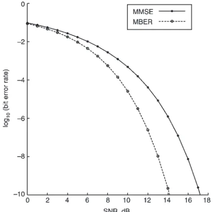
d¼3: Figure 1 compares the BER performance of the MMSE equaliser with that of the MBER one.Table 1lists the MMSE and MBER solutions, wMMSE and wMBER;

[image:4.612.46.267.386.604.2]

Fig. 1 Bit error rate performance comparison of the MMSE and MBER equalisers

Table 1: Weight vectors and BERs of the MMSE and MBER equalisers given SNR512 dB

MMSE MBER

w 0:162742þj0:084336 0:008256j0:008298

0:082974þj0:365218 0:131712þj0:175459

0:635619þj0:194423 0:636324þj0:349129

0:338643þj0:022754 0:535888þj0:292630

0:151703þj0:010665 0:212291j0:083981

BER 4:15105 2:49107

The weight vector has been normalised to a unit length

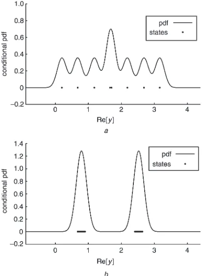
Fig. 2 Conditional probability density functions and subsets

YðþÞR of the MMSE and MBER equalisers for SNR¼12 dB The equaliser weight vector has been normalised to a unit length

a MMSE

[image:4.612.309.526.453.731.2] [image:4.612.35.276.675.779.2]

(5)

together with the associated BERs given SNR¼12dB: FromTable 1, it can be seen thatwMMSEandwMBERare very

different. The conditional pdf of the real part of the MMSE equaliser output, givenbðkdÞ ¼ þ1 and with aSNR¼ 12dB; is compared with that of the MBER equaliser in Fig. 2. For this example, the subsetYðþÞR containsNsb¼64

points. In Fig. 2 the equaliser weight vector has been normalised to a unit length, so that the BER is mainly determined by the minimum distance from the subsetYðþÞR

to the decision thresholdyR¼0:It can be seen fromFig. 2

that the minimum distance betweeny_R ¼0 andYðþÞ_R for the MMSE equaliser is smaller than that for the MBER equaliser. Also, the density distribution of yRðkÞ for the

MMSE equaliser is broader than that for the MBER equaliser. This means that the noise e(k) at the MMSE equaliser output has a larger variance. These two factors explain why the MMSE equaliser has a higher BER than the MBER equaliser.

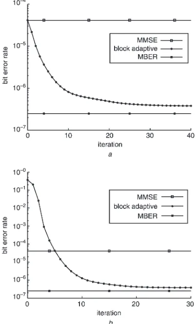
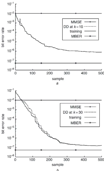
[image:5.612.328.536.325.694.2]

The performance of the block-data based adaptive MBER algorithm employing the conjugate gradient updating mechanism, as described in Section 4.1, was next studied. Figure 3 illustrates the convergence rate of the algorithm underSNR¼12dBand given two different initial weight vector conditions, where the block size wasK¼200:From Fig. 3, it can be seen that the convergence speed of this block-data gradient adaptive MBER algorithm is rapid. The performance of the stochastic gradient adaptive MBER algorithm discussed in Section 4.2 was then investigated. Figure 4 shows the learning curves of the algorithm

averaged over 30 runs, given SNR¼12dB and two different initial weight vector conditions. From Fig. 4, it can be seen that this stochastic gradient adaptive MBER algorithm has a reasonable convergence rate. There are in fact two learning curves in each of Figs. 4a and 4b, corresponding to training and decision directed (DD) adaptation in which bðkdÞ is substituted by the equaliser’s estimate bb^ðkdÞ: In Fig. 4a, the initial BER is well below the level of 104;and the two learning curves are indistinguishable. It can also be seen that, once the BER is below a certain level (typically 0.01), decision-directed adaptation can be applied with little performance degra-dation, as is confirmed inFig. 4b.

5.2 Adaptive beamforming assisted receiver

The ever-increasing demand for mobile communication capacity has motivated the employment of space division multiple access for the sake of improving the achievable spectral efficiency. A particular approach that has shown real promise in achieving substantial capacity enhance-ments is the use of adaptive antenna arrays. Adaptive beamforming is capable of separating signals transmitted on the same carrier frequency, provided that they are separated

Fig. 3 Convergence rate of the block-data gradient adaptive MBER algorithm for the equalisation example given SNR¼12 dB; and with a block size K¼200;step sizem¼0:9 and square width

r2

n¼32n0:14

a wð0Þ ¼wMMSE

b wð0Þ ¼ ½0:1þj0:0 0:1þj0:0 0:1þj0:0 0:1þj0:0 0:1þj0:0T

Fig. 4 Learning curves of the stochastic gradient adaptive MBER algorithm averaged over 30 runs for the equalisation example given SNR¼12 dB;where DD denotes decision directed adaptation withbb^ðkdÞsubstituting bðkdÞ

Ina, the two learning curves corresponding to training and DD adaptation are indistinguishable

a wð0Þ ¼wMMSE;step sizem¼0:1 and square widthr2n¼32n0:14 b wð0Þ ¼ ½0:1þj0:0 0:1þj0:0 0:1þj0:0 0:1þj0:0 0:1þj0:0T_; step sizem¼0:3 and square widthr2

[image:5.612.70.271.389.721.2]

(6)

in the spatial domain. Consider the system that supportsM

users (sources) which transmit on the same carrier frequency o¼2pf; and assume that the channel is

narrowband which does not induce intersymbol

interference. The linear antenna array considered consists ofLuniformly spaced elements, and the signals received by theL-element antenna array can be expressed in the form of (2), where theLM system matrixPis defined by

P¼ ½A0s0 A1s1 AM1 sM1 ð34Þ A2_i denotes the signal power of useri, and the steering vector for sourceiis given by

s_i¼ ½expðjot0ð iÞÞ expðjot1ð iÞÞ expðjotL1ð iÞÞ T

ð35Þ

withtlð iÞbeing the relative time delay at array elementlfor

source i and i the direction of arrival for source i. The

transmitted user symbol vector is bðkÞ ¼ ½b₀ðkÞb₁ðkÞ

bM1ðkÞT: Without any loss of generality, source 0 is

assumed to be the desired user and the rest of the sources are the interfering users. The desired user’s signal to noise ratio is defined as SNR¼A2₀=22n and the desired signal to

interference ratio with respect to interfering useriis defined asSIRi¼A20=A

2

i for 1iM1:The beamformer at the

receiver is a linear filter in the form of (1) withd¼0 in the decision rule (3).

[image:6.612.49.263.113.229.2]

The simulation example used consisted of six signal sources and a three-element antenna array.Figure 5shows the locations of the desired source and the interfering sources graphically.Figure 6 compares the BER perform-ance of the MMSE beamforming solution with that of the MBER one under two different conditions: (a) the desired user and all the five interfering sources had equal power, and (b) the desired user and the interfering sources 1, 3, 4, 5 had equal power, but the interfering source 2 had 6 dB higher power than the desired user. Note that when the 2nd interfering user’s power is increased by 6 dB, the MMSE beamformer’s performance breaks down, while the per-formance of the MBER beamformer remains almost unchanged. Thus, the MBER beamformer is robust to the so-called near – far effect.Tables 2 and 3list the MMSE and MBER solutions together with the associated BERs given a fixedSNR¼14dBand under the two given SIR conditions, respectively. Examining the two weight vectors for the

Table 2: Weight vectors and BERs of the MMSE and MBER beamformers given SNR514 dB and SIRi50 dB

for 1i5

MMSE MBER

w 0:170769j0:053050 0:448072j0:060545

0:186144j0:000000 0:783087j0:035493

0:170769þj0:053050 0:425536þj0:000000

BER 1:00102 ₅_:₄₀₁₀8

[image:6.612.50.264.286.741.2]

Table 3: Weight vectors and BERs of the MMSE and MBER beamformers given SNR514 dB;SIRi50 dB for

i51;3;4;5;and SIR₂56 dB

MMSE MBER

w 0:159405þj0:009740 0:450894j0:057414

0:120395j0:000000 0:783001j0:030264

0:159405j0:009740 0:423547j0:000000

BER 1:25101 5:60108

Fig. 5 Locations of the desired source and the interfering sources with respect to the three-element linear antenna array havingl=2 element spacing, wherelis the wavelength

Fig. 6 Bit error rate performance comparison of the MMSE and MBER beamformers

a SIRi¼0dBfor 1i5

[image:6.612.300.538.554.632.2] [image:6.612.299.538.702.778.2]

(7)

MBER solution under the two different conditions, they are very similar. However, differences between the two weight vectors of the MMSE solution can be clearly seen from Tables 2 and 3.Figures 7 and 8depict the conditional pdfs of the MMSE and MBER beamformers givenb0ðkÞ ¼ þ1

together with the associated subsets YðþÞR ; under the same

two conditions as given inTables 2 and 3. Again, in these two figures, the beamformer weight vector had been normalised to a unit length. It is interesting to see that, givenSNR¼14dB;SIRi¼0dBfori¼1;3;4;5 andSIR2

¼ 6dB; the resulting YðÞR and Y ðþÞ

R for the MMSE

beamforming becomes linearly inseparable. There areNsb

¼32 points inYðþÞR ;and a cluster of four points is on the

wrong side of the decision boundaryyR¼0 for the MMSE

beamforming, giving rise to a high BER floor 4=32¼ 0:125:

Performance of the block-data gradient adaptive MBER algorithm portrayed in Section 4.1 was next tested.Figure 9 illustrates the convergence rates of the algorithm givenSNR ¼14dB andSIRi¼0dB for 1i5;and with the two

different initial weight vectors. It can be seen that this block-data adaptive MBER algorithm generally converges rapidly. As the BER surface is highly complicated, the initial condition will influence convergence rate. It has been found out in a variety of applications that the MMSE solution

wMMSEis typically not a good initial choice for the adaptive

MBER algorithm in terms of convergence rate. Performance Fig. 7 Conditional probability density functions and subsets

YðþÞR of the MMSE and MBER beamformers given SNR¼14 dB and SIRi¼0 dB for 1i5

The beamformer weight vector has been normalised to a unit length

a MMSE

b MBER

Fig. 8 Conditional probability density functions and subsetsYðþÞR of the MMSE and MBER beamformers given SNR¼14 dB; SIRi¼0 dB for i¼1;3;4;5;and SIR2¼ 6 dB

The beamformer weight vector has been normalised to a unit length

a MMSE

b MBER

Fig. 9 Convergence rate of block-data gradient adaptive MBER algorithm for the beamforming example given SNR¼14 dB and SIRi¼0 dB for 1i5;and with a block size K¼200;step size

m¼0:6 and a square widthr2

n¼4n20:08

a wð0Þ ¼wMMSE

[image:7.612.68.274.50.331.2] [image:7.612.326.540.369.721.2] [image:7.612.65.279.431.724.2]

(8)

of the stochastic gradient adaptive MBER algorithm described in Section 4.2 was also investigated.Figure 10 shows the learning curves of the algorithm under the same conditions of Fig. 9, where DD denotes decision-directed adaptation with bb^0ðkÞ; substituting b0ðkÞ as the desired

response. It can be seen that this stochastic gradient adaptive MBER algorithm has a reasonable convergence speed. Note that the steady-state BER misadjustment is higher when the initial weight vector is set to w_MMSE; compared with the other initial weight condition.

6 Extension to nonlinear filtering

For a linear filter to work satisfactorily in a communication application, an implicit assumption is thatXðþÞ andXðÞ defined in (5) are linearly separable. That is, there exists a weight vectorwsuch that the two resulting scalar setsYðþÞR

andYðÞR are completely separated by the decision threshold yR ¼0:Otherwise nonlinear filtering is required. Examples

of such a nonlinear filtering includes nonlinear single-user equalisation and nonlinear multiuser detection[28 – 31]. If the linear restriction is removed, it can readily be shown that the true optimal filtering solution in terms of BER is the maximum a posteriori probability or Bayesian one, which is formulated as

yBðkÞ ¼

1

Nbð2p2nÞ L

XNb

q¼1

sgnðbq;dÞexp

kxðkÞ xxqk2

22 n

!

ð36Þ

wherexxq2 X andsgnðbq;dÞacts as a class label. Note that yBðkÞis real-valued due to its pdf interpretation, butx(k) and

x

xqare complex-valued. Because the number of vector states Nb is generally very large, this optimal Bayesian filtering

solution is computationally very expensive. In an adaptive implementation, all the states xxq have to be identified by

some means.

Consider the general nonlinear filter, which takes the form

yðkÞ ¼fðxðkÞ;wÞ ð37Þ

where the nonlinear mapfis generally complex-valued and is realised, for example, by a neural network, and the vector

wconsists of all the adjustable parameters of the nonlinear filter. Classically, adaptive training of such a nonlinear structure is based on the MMSE principle. For example, sample-by-sample adaptation is typically implemented using the LMS algorithm

yðkÞ ¼fðxðkÞ;wðk1ÞÞ

wðkÞ ¼wðk1Þ þmðbdðkÞ yðkÞÞ

@fðxðkÞ;wðk1ÞÞ

@w

ð38Þ

However, the true performance criterion of the system is the BER, and ideally the system design should be based on minimising the BER.

By linearising the nonlinear filter (37) aroundxxðkÞ;it can be approximated as

yðkÞ yyðkÞ þeðkÞ ð39Þ

where

y

yðkÞ ¼fðxxðkÞ;wÞ ð40Þ

can only take the value from the set

~ Y

Y ¼Df~yyq¼fðxxq;wÞ; 1qNbg ð41Þ

and

eðkÞ ¼ @fðxxðkÞ;wÞ @x

H

nðkÞ ð42Þ

is Gaussian with zero mean and variance

~ r r2nðwÞ ¼

22 n Nb

XNb

q¼1

@fðxxq;wÞ

@x

H

@fðxxq;wÞ

@x ð43Þ

The pdf ofyRðkÞcan then be approximated by

pðyRÞ

1

Nb

ffiffiffiffiffiffiffiffiffiffiffiffiffiffiffiffiffi 2prr~2

nðwÞ

p X

Nb

q¼1

exp ðyRyy~R;qÞ

2

2rr~2 nðwÞ

! ð44Þ

and the BER of the nonlinear filter is

PEðwÞ

1

Nb XN_b

q¼1

QðgqðwÞÞ ð45Þ

with

gqðwÞ ¼

sgnðbq;dÞyy~R;q

~ r rnðwÞ

¼sgnðbq;dÞfRðxxq;wÞ ~

r rnðwÞ

ð46Þ

Using the kernel density estimate in the form of (24) with a constantr2n to approximate the density (44) naturally leads

[image:8.612.54.254.46.376.2]

to a block-data based gradient adaptive near the MBER algorithm for training the nonlinear filter (37). This can be further simplified to give rise to a stochastic gradient adaptive near MBER algorithm in the form:

Fig. 10 Learning curves of stochastic gradient adaptive MBER algorithm averaged over 30 runs for the beamforming example given SNR¼14 dB and SIRi¼0 dB for 1i5; where DD denotes decision directed adaptation withbb^0ðkÞsubstituting b0ðkÞ

a wð0Þ ¼wMMSE;step sizem¼0:03 and square widthr2n¼22n0:04 b wð0Þ ¼ ½0:1þj0:0 0:1þj0:0 0:1þj0:0T_;_{step size}_m_¼₀_:_{02 and} square widthr2

(9)

yðkÞ ¼fðxðkÞ;wðk1ÞÞ

wðkÞ ¼wðk1Þ þmsgnðbdðkÞÞ

2pffiffiffiffi2prn

exp y2RðkÞ

2r2

n

_@_f

RðxðkÞ;wðk1ÞÞ

@w

)

ð47Þ

for a sample-by-sample adaptation. The derivative@fR=@w

depends on the particular nonlinear map employed. Previous studies [32 – 34] have applied this adaptive near MBER nonlinear filtering approach to equalisation and multiuser detection applications.

7 Conclusions

A general adaptive filtering technique has been proposed for applications to communication systems based on the novel MBER principle. It has been demonstrated that the MBER filtering is capable of achieving significant performance gains in terms of reduced BER over the traditional MMSE filtering. Adaptive implementation of the proposed MBER filtering has been developed based on the classical Parzen window estimation for the pdf of the filter’s output. A block-data based conjugate gradient adaptive MBER algorithm has been shown to converge rapidly and requires a reasonably small data block size to accurately approximate the theoretical MBER solution. An LMS-style stochastic gradient adaptive MBER algorithm has been shown to perform well, and the algorithm has similar computational requirements to the low-complexity LMS algorithm. Extension of this adaptive MBER filtering approach to nonlinear filtering has been discussed.

8 Acknowledgment

Original contributions of Professor B. Mulgrew to the topic of adaptive MBER equalisation are gratefully acknowledged.

9 References

1 Widrow, B., and Stearns, S.D.: ‘Adaptive signal processing’ (Prentice-Hall, Englewood Cliffs, NJ, 1985)

2 Haykin, S.: ‘Adaptive filter theory’ (Prentice-Hall, Upper Saddle River, NJ, 1996, 3rd edn.)

3 Shamash, E., and Yao, K.: ‘On the structure and performance of a linear decision feedback equalizer based on the minimum error probability criterion’. Proc. ICC, 1974, pp. 25F1 – 25F5

4 Chen, S., Chng, E.S., Mulgrew, B., and Gibson, G.: ‘Minimum-BER linear-combiner DFE’. Proc. ICC, Dallas, Texas, 1996, vol. 2, pp. 1173 – 1177

5 Yeh, C.C., and Barry, J.R.: ‘Approximate minimum bit-error rate equalization for binary signaling’. Proc. ICC, Montreal, Canada, 1997, vol. 2, pp. 1095 – 1099

6 Chen, S., Mulgrew, B., Chng, E.S., and Gibson, G.: ‘Space translation properties and the minimum-BER linear-combiner DFE’,IEE Proc., Commun., 1998,145, (5), pp. 316 – 322

7 Chen, S., and Mulgrew, B.: ‘The minimum-SER linear-combiner decision feedback equalizer’, IEE Proc., Commun., 1999,146, (6), pp. 347 – 353

8 Mulgrew, B., and Chen, S.: ‘Stochastic gradient minimum-BER decision feedback equalisers’. Proc. IEEE Symposium on Adaptive systems for signal processing, communication and control, Lake Louise, Alberta, Canada, 1 – 4 Oct. 2000, pp. 93 – 98

9 Yeh, C.C., and Barry, J.R.: ‘Adaptive minimum bit-error rate equalization for binary signaling’,IEEE Trans. Commun., 2000,48, (7), pp. 1226 – 1235

10 Mulgrew, B., and Chen, S.: ‘Adaptive minimum-BER decision feedback equalisers for binary signalling’,Signal Process., 2001,81, (7), pp. 1479 – 1489

11 Mandayam, N.B., and Aazhang, B.: ‘Gradient estimation for sensitivity analysis and adaptive multiuser interference rejection in code-division multi-access systems’, IEEE Trans. Commun., 1997, 45, (7), pp. 848 – 858

12 Yeh, C.C., Lopes, R.R., and Barry, J.R.: ‘Approximate minimum bit-error rate multiuser detection’. Proc. Globecom, Sydney, Australia, Nov. 1998, pp. 3590 – 3595

13 Wang, X.F., Lu, W.S., and Antoniou, A.: ‘Constrained minimum-BER multiuser detection’. Proc. ICASSP, Phoenix, USA, 14 – 18 May 1999, vol. 5, pp. 2603 – 2606

14 Psaromiligkos, I.N., Batalama, S.N., and Pados, D.A.: ‘On adaptive minimum probability of error linear filter receivers for DS-CDMA channels’,IEEE Trans. Commun., 1999,47, (7), pp. 1092 – 1102 15 Chen, S., Samingan, A.K., Mulgrew, B., and Hanzo, L.: ‘Adaptive

minimum-BER linear multiuser detection’. Proc. ICASSP, Salt Lake City, Utah, USA, 7 – 11 May 2001, vol. 4, pp. 2253 – 2256

16 Chen, S., Samingan, A.K., Mulgrew, B., and Hanzo, L.: ‘Adaptive minimum-BER linear multiuser detection for DS-CDMA signals in multipath channels’, IEEE Trans. Signal Process., 2001, 49, (6), pp. 1240 – 1247

17 Chen, S., Ahmad, N.N., and Hanzo, L.: ‘Smart beamforming for wireless communications: a novel minimum bit error rate approach’. Proc. 2nd IMA Int. Conf. on mathematics in communications, Lancaster, UK, 16 – 18 Dec. 2002

18 Chen, S., Hanzo, L., and Ahmad, N.N.: ‘Adaptive minimum bit error rate beamforming assisted receiver for wireless communications’. Proc. ICASSP, Hong Kong, China, 6 – 10 April 2003, vol. IV, pp. 640 – 643 19 Chen, S., Ahmad, N.N., and Hanzo, L.: ‘Adaptive minimum bit error

rate beamforming’, submitted to IEEE Trans. Wireless Communi-cations, 2002

20 Parzen, E.: ‘On estimation of probability density function and mode’,

Ann. Math. Stat., 1962,33, pp. 1066 – 1076

21 Silverman, B.W.: ‘Density estimation’ (Chapman Hall, London, 1996) 22 Bowman, A.W., and Azzalini, A.: ‘Applied smoothing techniques for

data analysis’ (Oxford University Press, Oxford, 1997)

23 Chen, S., Mulgrew, B., and Hanzo, L.: ‘Stochastic least-symbol-error-rate adaptive equalization for pulse-amplitude modulation’. Proc. ICASSP, Orlando, Florida, USA, 13 – 17 May 2002, vol. 3, pp. 2629 – 2632

24 Chen, S.: ‘Minimum symbol-error-rate equalisation’. Proc. EPSRC/IEE Non-linear and non-Gaussian signal processing workshop, Peebles, Scotland, 8 – 9 July 2002

25 Chen, S., Hanzo, L., and Mulgrew, B.: ‘Adaptive minimum symbol-error-rate decision feedback equalization for multi-level pulse-ampli-tude modulation’, submitted toIEEE Trans. Signal Processing, 2002 26 Bazaraa, M.S., Sherali, H.D., and Shetty, C.M.: ‘Nonlinear

program-ming: theory and algorithms’ (John Wiley, New York, 1993) 27 Sharma, R., Sethares, W.A., and Bucklew, J.A.: ‘Asymptotic analysis of

stochastic gradient-based adaptive filtering algorithms with general cost functions’,IEEE Trans. Signal Process., 1996,44, (9), pp. 2186 – 2194 28 Chen, S., Mulgrew, B., and Grant, P.M.: ‘A clustering technique for digital communications channel equalisation using radial basis function networks’,IEEE Trans. Neural Netw., 1993,4, (4), pp. 570 – 579 29 Chen, S., Mulgrew, B., and McLaughlin, S.: ‘Adaptive Bayesian

equaliser with decision feedback’,IEEE Trans. Signal Process., 1993,

41, (9), pp. 2918 – 2927

30 Chen, S., McLaughlin, S., Mulgrew, B., and Grant, P.M.: ‘Bayesian decision feedback equaliser for overcoming co-channel interference’,

IEE Proc., Commun., 1996,143, (4), pp. 219 – 225

31 Chen, S., Samingan, A.K., and Hanzo, L.: ‘Support vector machine multiuser receiver for DS-CDMA signals in multipath channels’,IEEE Trans. Neural Netw., 2001,12, (3), pp. 604 – 611

32 Chen, S., Mulgrew, B., and Hanzo, L.: ‘Adaptive least error rate algorithm for neural network classifier’. Proc. IEEE Workshop on Neural networks for signal processing, Falmouth, MA, USA, 10 – 12 Sept. 2001, pp. 223 – 232

33 Chen, S.: Mulgrew, B., and Hanzo, L.: ‘Least bit error rate adaptive nonlinear equalizers for binary signalling’,IEE Proc., Commun., 2003,

150, (1), pp. 29 – 36

34 Chen, S.: ‘Least bit error rate adaptive multiuser detection’, in Wang, L.P. (Ed.): ‘Soft computing in communications’ (Springer Verlag, 2003), pp. 389 – 408

10 Appendix

The conditional pdf ofyRðkÞgivenbdðkÞ ¼ þ1 is

pðyRjþÞ ¼

1

Nsb

nwHw

p X

Nsb

q¼1

exp

yRyy ðþÞ R;q

2

22 nwHw 0

B @

1 C A

ð48Þ

whereyyðþÞ_R_;_q 2 YðþÞR :Thus the conditional BER of the linear

filter (6) givenbdðkÞ ¼ þ1 is

PE;þðwÞ ¼ Z 0

1

pðyRjþÞdyR¼

1

Nsb XNsb

q¼1

(10)

gq;þðwÞ ¼

y yðþÞ_R_;_q

_npffiffiffiffiffiffiffiffiffiffiwH_w¼

sgnðbq;dÞyy ðþÞ R;q

_npffiffiffiffiffiffiffiffiffiffiwH_w

¼sgnðbq;dÞR½w

H_x_xðþÞ q

p ð50Þ

QðxÞ ¼ 1ffiffiffiffiffiffi 2p p

Z 1

x

exp u

2

du ð51Þ

Similarly, the conditional pdf ofyRðkÞgivenbdðkÞ ¼ 1 is

pðyRjÞ ¼

1

Nsb

nwHw

p X

N_sb

q¼1

exp

yRyy ðÞ R;q

2

22 nwHw 0

B @

1 C A

ð52Þ

whereyyðÞ_R_;_q 2 YðÞR ;and the conditional BER givenbdðkÞ ¼

1 is

PE;ðwÞ ¼ Z 1

0

pðyRjÞdyR ¼

1

Nsb XNsb

q¼1

Qðgq;ðwÞÞ ð53Þ

with

gq;ðwÞ ¼

y yðÞ_R_;_q

_npffiffiffiffiffiffiffiffiffiffiwH_w¼

sgnðbq;dÞyy ðÞ R;q

_npffiffiffiffiffiffiffiffiffiffiwH_w

¼sgnðbq;dÞR½w

H_x_xðÞ q

p ð54Þ

Because of the symmetric distribution of YR;PE;ðwÞ ¼ PE;þðwÞ:This proves that the BER of the linear filter with a

weight vectorwis given by

PEðwÞ ¼

1

2PE;þðwÞ þ 1

2PE;ðwÞ

¼ 1

Nsb XNsb

q¼1

It is also obvious that the BER can be expressed as

PEðwÞ ¼

1

Nb XNb

q¼1

QðgqðwÞÞ ð56Þ

where

gqðwÞ ¼

sgnðbq;dÞyyR;q

p ¼sgnðbq;dÞR½w

H_x_x q

p ð57Þ