A comprehensive and robust procedure for obtaining the nofit polygon using Minkowski sums

A comprehensive and robust procedure for obtaining the nofit polygon

using Minkowski sums

JULIA A BENNELL

School of Management, University of Southampton, Southampton SO17 1BJ, United Kingdom, [email protected]

XIANG SONG

School of Management, University of Southampton, Southampton SO17 1BJ, United Kingdom, [email protected]

The nofit polygon an important tool in the area of irregular shape stock cutting problems. It provides efficient handling of the geometric characteristics of the problem. The paper presents a new algorithmic procedure for deriving this tool.

Submitted: June 2005

Abstract

1. INTRODUCTION

The paper specifically addresses the geometric calculations required for tackling cutting and packing problems involving irregular shapes. Such problems are common in manufacturing processes and occur whenever a piece of irregular shape is to be cut from a sheet of stock material. Examples include dye-cutting in the engineering sector, parts nesting for shipbuilding, marker layout in the garment industry, and leather cutting for shoes, furniture and other goods. Here we consider that shapes are irregular if they are; polygonal, i.e no arcs; simple, i.e. do not self-cross; and non-rectangular. Even when all the components are rectangular the problem of finding layouts that minimize waste is known to be NP-hard. Where irregular components are involved an extra dimension of complexity is generated by the geometry.

Although all these approaches have merit, it is widely recognized that the nofit polygon (NFP) is more efficient, provided you have a robust and efficient NFP generator, and has become the principle approach for handling the geometry in nesting problems. Unfortunately, some researchers believe that despite the value of this tool, its introduction may have stifled research into this variant of packing problems. Wäscher, Haußner and Schumann (2005) reports that there have been only 21 publications in irregular problems in the last 10 years. Researchers attribute this to the fact that the realization of the NFP as a robust algorithm is, in itself, a highly challenging task. Those considering embarking on research into irregular shaped packing may be discouraged by the significant investment of time required in first developing an NFP generator. Hence, it is essential that robust and easily realizable algorithms are available in order to facilitate new interest into this important problem.

the modification required in order to determine the inner-fit polygon. Finally, we develop some theoretical and empirical analysis of the approach to demonstrate its robustness.

2. DOCUMENTED APPROACHES FOR GENERATING THE NOFIT

POLYGON

approaches to generating the NFP; the orbiting method that simulates the sliding motion, and Minkowski sums that sort the edges according to the the slope order and edge precedence, i.e the sequential order of edges around the polygons. A further approach commonly employed is that of decomposition. A brief description of each is provided here.

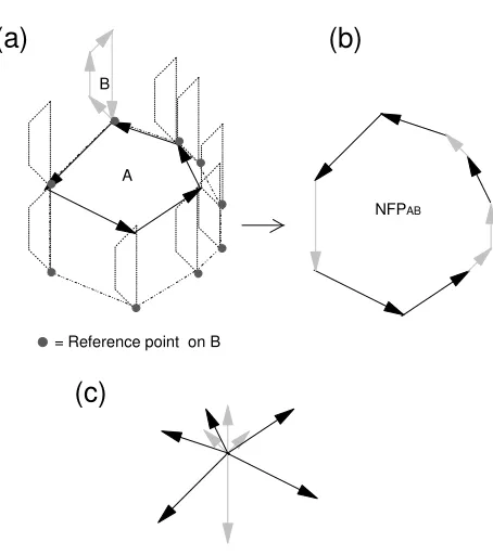
Figure 1: The locus of the reference point on B traces the NFP as it slides around A. This is equivalent to connecting the edges in slope order.

Minkowski sum

Clearly, when both component polygons are convex the NFP is very simple to calculate by sorting the edges into slope order. Further, when one of the polygons is

(b)

(c)

(a)

B

NFPAB A

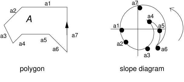
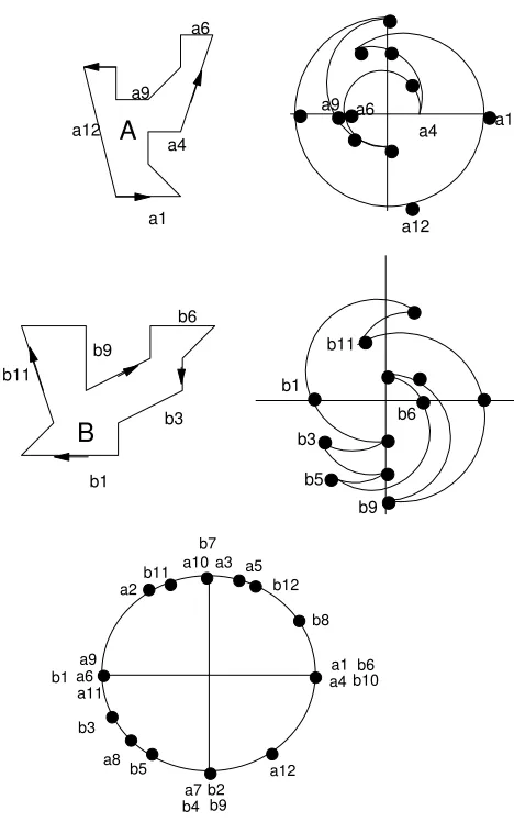
convex and the other is an arbitrary simple polygon, the NFP can still be easily obtained from the slope order and the precedence of the edges. In this case, the NFP is obtained by forming an edge list that follows the precedence of the simple polygon, assigned as polygon A, in a counterclockwise direction, and adding the edges of the convex polygon, assigned polygon B, to the list whenever they are encountered in the slope order. Due to the concavities in A, the precedence will necessitate a clockwise turn through the slope order, if the edges of the convex polygon are encountered in the clockwise direction; they are included in the edge list with negative direction. Note that this also retains the precedence of the edges of the convex polygon. Unfortunately the resulting polygon created from this edge list is complex and further computation is required to remove edges or parts of edges that are not part of the boundary of the NFP. Figure 2 illustrates the tracking of the precedence order of a simple polygon through the slope order.

Figure 2: A simple polygon and respective slope order

It is worth noting that even in the convex-simple case, the NFP may contain holes. a2

a4 a5

a3 a6

a7

a1 a1

a3

a4 a5

a6 a7 a2

A

encountered through sliding. Such cases will be discussed later in the paper. When both polygons contain concavities, following the precedence of both polygons, simultaneously, becomes impossible without further modification to the approach. Since it is these principles that form the basis of the Minkowski sum approaches presented in this paper, these issues will be discussed in later sections.

Orbiting method

candidates for possible holes. A process of identifying all feasible touching start position is performed for the candidate edges. If a feasible start position is found, the sliding approach is performed again from that starting point. This continues until all edges not flagged have been investigated.

Decomposition

Given the comparative complexities of the described approaches when one or both polygons are simple, decomposing the component polygons into suitable sub-polygons is an attractive option. Examples in cutting and packing literature include convex decomposition (Watson and Tobias, 1999) and star shaped decomposition (Li and Milenkovic, 1995). As previously described, the NFP of two convex polygons is trivial. Li and Milenkovic selected star shaped polygons since the NFP of two star shaped polygons is also star shaped. Hence, in generating the sub-NFP, they need only be concerned with the outer boundary.

Flato and Halperin (2002) found that the recombination operation was the most computationally expensive and report relatively high computation times.

A recent development in handling the geometric properties of irregular packing problems, in both two and three dimensions, is that of the Phi-function (Stoyan et al, 2001, 2002). Although phi-functions are not strictly nofit polygons, they are a related concept and have proved to be both efficient and effective. The Phi-function is able to determine the distance between two polygons and therefore whether they overlap. Stoyan et al analytically construct phi-functions for all primary objects; rectangles, circles and other convex polygons. As a result, arbitrary polygons or parallelepipeds can be handled by representing them as a finite combination (union, intersection, complement) of primary objects.

All of the methods described have been somewhat successful. However, all experience difficulties when; the problem instance becomes complex, for example, degenerate cases where one or more dimension fits exactly into a concavity; computational times can be large; and the algorithm proposed difficult to realize. In this paper we will further develop the Minkowski sum approach and present a robust, efficient and simple algorithm. Although we do not dismiss the potential of the other approaches, a clear advantage of this approach is that the basic Minkowski sum can be obtained through simple rules designed to list the edges according to the precedence of both polygons while sorting in slope order. For all the described methods, the identification of holes and degenerate cases is somewhat laborious.

3. APPROCHES TO FINDING THE NOFIT POLYGON USING MINKOWSKI

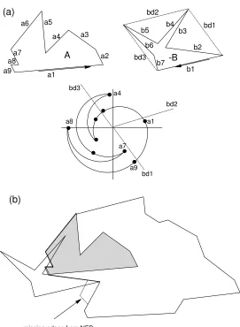
As previously described, generating the NFP of both the convex-convex and simple-convex case can easily be solved using the slope and precedence order of the edges. Ghosh (1991, 1993) developed these ideas and proposed the theory of boundary addition, which can be illustrated through the use of a slope diagram. Figure 3a illustrates two polygons converted into their respective slope diagrams. Note that the polygons have opposite orientation, A has counter clockwise orientation; positive, and B has clockwise orientation; negative. The boundary addition theorem states that the Minkowski sum,

B

Figure 3 Ghosh (1991) approach to two simple polygons with interacting concavities

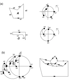
Bennell, Dowsland and Dowsland (2001) propose an alternative approach to the simple-simple case. Their approach exploits the knowledge that the simple-convex case is trivial and that the Minkowski sum of a simple polygon A with the convex hull of polygon B, MinkAconv(B) , will contain all the boundary and internal points of the original simple-simple case, MinkAB. In order to generate conv(B), dummy edges are introduced that replace the edges that make up the concavities of B. Clearly these dummy edges

b1 b2 b3 b4 -B b1 b2 b3 b4 b5 b5 (a) b3 a4 a5 a3 a2 a1 b2 -b4 b5 b1 -a3 a3 a4 a3 a4 -a4 b3 b4 b4 -b3 b3 b4

appear, both positively and negatively, in MinkAconv(B). Hence replacing the dummy edges in the edge list of MinkAconv(B) by the real edges of B, following the precedence of the edges and including A edges when they are passed in the slope order, will result in MinkAB.

While Bennell, Dowsland and Dowsland’s approach works well on the benchmark data sets (ESICUP), further investigation highlights some ambiguity in the procedure for replacing dummy edges. This is illustrated through the example in figure 4.

Figure 4(a) illustrates the generation of MinkAconv(B). It is clear that dummy edge bd1

will slide across the vertex between edge a9 and edge a1 . Hence appearing on the slope

diagram on that traversal alone. However, we can observe in figure 4(b) that vertex (a9,a1) can not slide along the full extent of edge b2 due to a collision between edge b3

and vertex (a6,a7). However, if when replacing the dummy edge in the slope diagram,

-B a2 a3 a5 a6 a9 b2 b3 b4 b5 b6 b7 b1 a1 a4 a7 a8 bd2 bd1 bd3 A

missing edges from NFP

(a) (b) a4 a7 a9 a1 bd2 bd1 bd3 a8

Figure 4 An example when edges may be missed when using Bennell, Dowsland and Dowsland (2001)

4. A REVISED PROCEDURE FOR OBTAINING THE BOUNDARY OF THE

NOFIT POLYGON

edges should be included in the edge list. The basic idea is to break polygon B into groups that are in either continuous counter clockwise or clockwise order. Each of the groups can then be individually merged with the slope diagram of A without conflict. When combining the merged lists, linking edges need to be included in order to maintain the precedence of the edges in each polygon. As with Ghosh and Bennell, Dowsland and Dowsland, the resulting edge list is a complex polygon, where the edges represent all the boundary edges and some internal points of the Minkowski sum. In order to have successfully generated the NFP, the edges that are not part of the boundary must be removed. The approach for finding the Minkowski sum will be first illustrated by an example and then the algorithmic procedure will be given. Removal of internal edges will be addressed in the next section.

Consider the example previously given in figure 3. If we follow the precedence of A, traversing from a2 to a3 we will encounter b4 before b3, yet the previous B edge encountered had been b2. The equivalent conflict would occur in A if we followed the precedence of B. However, if we break polygon B at the vertex connecting b3 and b4, and consider the edges as a list, instead of a cycle, starting from b4, then we have b4, b5, b1,

The approach applied to the example in figure 3 works as follows. Start from the first B edge, b4, we search for b5. To find this we traverse a3 and a4. From b5 we search for b1 and traverse a5. From b1 we search for b2 and traverse a1. Finally we search for b3 traversing a2. Since b3 crosses the concavity of A, it will appear three times. This was established through the initial counting phase. Hence the search continues until all appearances of b3 have been found. Thus we obtain b4, a3, a4, b5, a5, b1, a1, b2, a2, b3, a3, -b3, a4, b3. Given that a polygon must be a complete cycle, we must now link the beginning and the end of the list. Hence from b3 we will look for b4. This requires a clockwise turn through the slope diagram traversing –a4 and –a3. Thus finally we obtain:

b4, a3, a4, b5, a5, b1, a1, b2, a2, b3, a3, -b3, a4, b3, -a4, -a3.

In summary, the procedure to form the sequence follows the slope diagram of A positively when the series of B edges are in a counter clockwise direction and follows it negatively when the series of B edges are in a clockwise direction. With this knowledge, we consider a more complex case.

1. b12, b1, b2 (counter clockwise) 2. b3, b4 (counter clockwise) 3. b5, b6, b7 (counter clockwise) 4. b8 (clockwise)

5. b9, b10, b11 (counter clockwise)

Figure 5: Complex case of two polygons with more than one concavity in each polygon

1. [a1], b12, a2, a3, -b12, a4, b12, a5, b1, a6, b2, a7, -b2, a8, -b1, a9, a10, b1, a11,

b2, -a11, -a10, -a9, -a7

2. [a6], b3, b4, a7, -b4, a8, -b3, a9, a10, a11, b3, b4, -a11, -a10, -a9, -a7

3. [a6], b5, a7, -b5, a8, a9, a10, a11, b5, a12, b6, a1, b7, a2, -b7, a3, -b6, a4, b6, a5, b7, a6, a7, a8, a9, -b7, a10, b7, -a10, -a9, -a7, -a6, -a5

4. [-a5], b8, -a4, -b8, -a3, -a2, b8, a2, a3, a4, a5

5. [a6], b9, a7, -b9, a8, a9, a10, a11, b9, a12, b10, a1, b11, a2, -b11, a3, -b10, a4,

b10, a5, b11, a6, a7, a8, a9, -b11, a10, b11, -a10, -a9, -a7, -a6, -a5, -a4, -a3, -a2

The procedure to find the Minkowski sum of two polygons A and B is given below. Note that if a group of B edges have continuous counter clockwise order, it is labeled as positive, otherwise it is labeled as negative. A positive group traverses the slope diagram of A in counter clockwise order including positive A edges. A negative group follows the slope diagram in clockwise order including negative A edges. Only the positive procedure is included here. For efficiency, the procedure in Mink(Q,R,positive) traverses the slope order list following the precedence of A recording the B edges encountered along the way to provide list, s. This process allows us to know the number of times each B edge is encountered and in what direction. Further list s can be used to create the correct sequence of A and B edges without searching the slope order a second time.

Algorithm 1: Algorithm to generate the Minkowski Sum

Step 1: Replace B by –B, i.e. replace all co-ordinates

(

)

(

)

Step 2: Starting at the lowest point on each polygon. Label the edges in counter clockwise order.

Calculate the angle θ

( )

If any turning points have been detected then polygon is non-convex. Sort the edges into angle order to form sort_list(P), where P = A or –B.

Step 3: Let

(

)

Then polygon B can be divided into groups B1=

(

)

B2=

(

)

(

)

consecutive counterclockwise direction or consecutive clockwise direction. Step 4: For each group Bj, (j =1,…, n), call Mink(A, Bj, positive) or Mink(A, Bj, negative)

according to group Bj being counter clockwise or clockwise respectively. We

obtain Seqj.

Step 6: Link Seq_list(A,B1),…,Seq_list(A,Bn) with additional A edges one by one. If Seq_list(A,Bj) is positive, insert negative A points to link Seqi with Seqi+1 .

else Seq_list(A,Bj) is negative, insert positive A points to link Seqi with Seqi+1 .

Mink(Q, R, positive).

Step 1 : merge sort_list(Q) and sort_list(R) to form merge_list(Q,R) Step 2: set i = 1, k = 1, direction = 1, s1 = q1

Step 3: Set i = i + 1

Search merge_list(Q,R) for qi moving forward if direction = 1 and backwards if direction = -1

if R edge, rj, set k = k + 1, sk = direction rj

When qi is encountered, if i = 1, go to step 4

If qi is a turning point in Q, set direction = - direction

Repeat step 3

Step 4: Let starting edge r1 be in position si in sequence

Set j = 1, next = 2, direction = 1, seq1 = si Step 5: Set i = i + 1, if i > k, set i = 1

If si is from Q, j = j + 1, seqj = si

If si is a turning point in Q, direction = - direction, next = next + direction

If si = direction.rnext, j = j + 1, seqj = si, next = next + direction

If all si edges have been allocated to seqj, return seq1 to seqj as Seq_list(Q,R)

Otherwise, repeat step 5

5. COMPUTING THE BOUNDARY OF THE NFP

The resulting Minkowski sum is a complex (self crossing) polygon where the edges include all the edges of the nofit polygon and some internal points. In this section we describe a new method for identifying the true edges of the NFP.

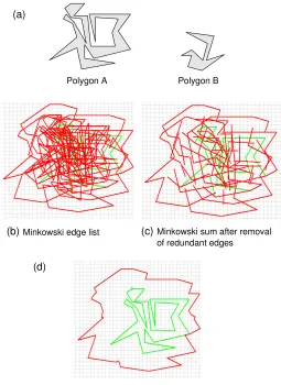
Figure 6b illustrates the outcome of the Minkowski sum procedure described in the previous section, for two simple polygons drawn in 6a. Clearly there are many edges to untangle. However, using some of the properties we know about the NFP and the boundary addition method we can quickly remove many of these edges.

Property 2. The slope diagram representation, used in boundary addition, indicates that if edge bj appears between edges (ai,ai+1), this corresponds to the physical condition

that edge bj slides along vertex (ai,ai+1). When the direction from ai to ai+1 is counter

clockwise and edge bj is positive, the corresponding sliding condition is that the convex

vertex (ai,ai+1) slides along bj. Otherwise, the negative edge bj corresponds to the

condition that the concave vertex (ai,ai+1) slides along edge bj. Clearly an edge cannot

slide along a concave vertex without creating overlap between the polygons.

It can be deduced from these two properties that any negative edges cannot be part of the boundary of the NFP and can be removed. Further, the linking edges between sequences can also be removed since their inclusion is to define the correct starting position of the next sequence and they do not represent potential sliding between the polygons. Figure 6c illustrates the Minkowski edge list with the redundant edges removed. With this understanding, we can develop intuitively a new method to identify the boundary of the NFP by only considering useful parts of the derived Minkowski sum edge list.

Figure 6: A large example of the Minkowski sum edge list and track line traces

In order to introduce this method, we recall briefly some terms introduced by Ramkumar (1996). A state is a pair consisting of a position s in the plane and a direction s. A move is a set of states with constant direction and position varying along a line segment parallel to the direction. A turn is a set of states with constant position and direction varying along an arc of the circle of directions. A polygonal trip consists of a continuous sequence of moves and turns; the trip is closed if it starts and ends at the same state. A polygonal tracing is a collection of closed polygonal trips. We think of each loop

Polygon B Polygon A

(a)

(b) Minkowski edge list (c) Minkowski sum after removal of redundant edges

of a tracing as being traversed by a car which always faces in the direction of the state it is currently following.

The first step is to break up the Minkowski sum into polygonal trips according to the continuous sequence of moves and turns. Those that cannot be part of the boundary of the NFP, according to the properties described above, are discarded. This is equivalent to removing the negative and additional A edges.

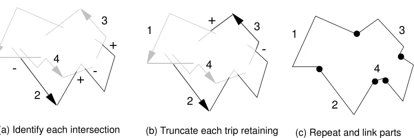
Figure 7: Procedure for removing internal edges from the Minkowsi sum

The second step of the procedure requires the identification of all the intersection points between the polygonal trips. Each intersecting point is marked with a ‘-’, indicating it is entering the trip, or with a ‘+’, indicating it is leaving the trip. Consider the example in figure 7a, where the current trip is trip 2. Imagine standing at the beginning of the first edge of trip 2 facing along the edge, then we can consider that trip 1 intersects trip 2 from right to left. Trip 1 is said to enter trip 2 and is marked with ‘-’. Continuing along trip 2 we eventually meet an intersection with trip 4, where trip 4 intersects from left to right. Trip 4 is leaving trip 2 and marked with ‘+’. Hence, entering

3 2 4 1

-+

-+

-+

(a) Identify each intersection

a trip means the beginning part of the intersecting edge is on the right side of the trip edge and leaving corresponds to the beginning part of the intersecting edge is on the left side of the trip edge. The fragments of trips that span a ‘-’ intersection to a ‘+’ intersection are kept to form the boundary of the NFP. All other fragments are discarded.

Finally, fragments that share end points are linked. Only those parts, which form a cycle, can be taken as the boundary of the NFP. In the case where cycles represent holes in the NFP, we implement a simple direct test of whether the two component polygons overlap when the reference point of B is located on a vertex of the hole.

The algorithm for finding the boundary of the nofit polygon can be summarized in Algorithm 2 and 3 as below:

Algorithm 2: Algorithm for breaking Minkowski sums into track line trips:

Step 1: Let i=0 be the index number of Minkowski sums obtained. Let j=0 be the number of track line trips, nj be the total edges in track line trip j and k =0 be the

index of each track line trip.

Step 2: Search forward in Minkowski Sum for positive si, which corresponds to a

track line. If si can be found, set tjk =si, else go to Step 4.

Step 3: Set i=i+1 and k =k +1. If si is positive and corresponds to a track line,

repeat step 3,

else set nj =k, j= j+1 and k=0, repeat Step 2.

The computational complexity of Algorithm 2 is O

( )

Algorithm 3: Algorithm for finding the boundary of the NFP from track line trips:

Step 1: Let trip Tj, contain segjnjsegments.

For all i and j where i≠ j,

Ifseg_jkj intersects seg_iki, let p_jrj be the intersection points on T_j

If pjr_j crosses right to left set signjrj =−1, else set signjrj =+1.

Step 2: For each Tj,

If signjr_j =−1 and signjrj+1 =+1. Store all segments between the intersection

points,

{

}

{

}

the number of segments in frag_i.

Step 3: For all fragi ≠0, we

if fi1= fjlj, fragi = fragj+ fragi =

{

}

if f_j1= f_ili, frag_i = frag_i+ frag_j =

{

}

if f_i1= f_jlj and f_j1= f_ili then form cycle_k and set frag_i = frag_j =0

Repeat step 3 until all fragi =0.

Step 4: For each cycle_k,

Locate reference point of polygon B on one of the vertexes of cycle_k.

It is important to note that the above algorithm is able to identify the outer face of the

Minkowski sums, holes inside the outer face, a single point that represent an exact fit, and

exact slides represented as a single line. The latter two are often referred to as degenerate

cases.

Degenerate cases

The degenerate cases, in general, refer to combinations of polygons that can fit together

like a jigsaw, resulting in a single point of fit within the NFP, or where one piece can

slide into or within a concavity in one direction only, resulting in a line either extending

from the edge of the NFP or within.

fragj fragi

d c

b a

(b)

d

c b

a

(c) (a)

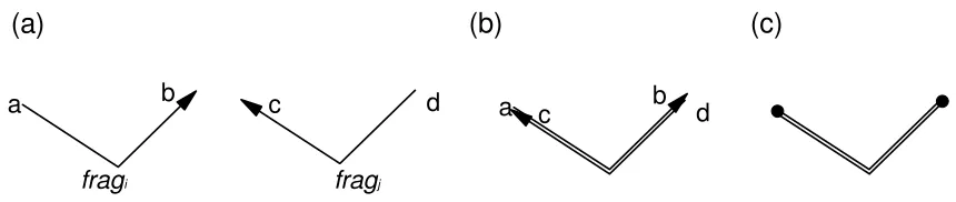
Figure 8: Coinciding fragments to indicate exact slide in NFP

An exact slide can be identified when two fragments, obtained from Algorithm 3, step

2, coincide. Figure 8a illustrate frag_i and frag_j with start points, a and d, and end

points, b and c respectively. If the start and end points from each fragment coincide, as

shown in figure 8b they can be linked into a cycle (figure 8c) in step 3. The cycle is

In the case of a single point, further calculation is required in Algorithm 3, step 1. When

all the intersection points between segments of the trip are calculated, we also identify

special intersection cases as shown in figure 9, where trips Ti and Tj intersect each other

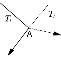
at point A. It is necessary to test all intersection points of this type to identify if it is an

exact fit. In our experience, intersection points such as A seldom occurred within the

intersection condition.

T

T

A

Figure 9: Edge intersection to indicate exact nesting point in NFP

6. THE INNER FIT POLYGON

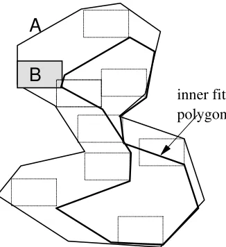
The inner fit polygon represents the feasible placement positions of one polygon, B,

inside another polygon, A. An example of this is given in figure 10. This is useful for

obstacle recognition in robot motion planning and if pieces are being packed inside an

A

B

inner fit polygon

Figure 10: An inner fit polygon

The described algorithm can be used to calculate the inner-fit polygon with the following

minor amendments.

(i) Reverse the orientation of polygon A so that it has clockwise direction.

(ii) The algorithm should have the positive direction for A as clockwise. However,

clockwise is still the negative direction for B

The rationale for these changes can be demonstrated in figure 11. The inner-fit polygon is

equivalent to B sliding inside a concavity of A. As illustrate in figure 11, the concavity

has clockwise orientation. Further a concavity translates to a clockwise turn in the slope

diagram where the edges of the concavity remain positive, while any edges from the

A

B

Figure 11: the equivalence between the inner-fit polygon and the NFP inside a concavity

7 EMPICICAL ANALYSIS

In order to evaluate the effectiveness of our new approach, we generated all the nofit

polygons for the benchmark data sets found on the ESICUP (2005) website. All were

generated correctly and the computation times for every combination of each data set are

provided in table 1. The procedure was coded in Visual Studio C++ and the instances

were run on a pc with 512MB, 1.6GHz.

No. CASE No. of piece types Ave no. of edges TIME (s)

1 Albino_hopper 8 7.25 0.07

2 Blaz_topos 7 6.28 0.04

3 Dagli_hopper 10 6.3 0.07

4 Dighe_hopper 10 4.7 0.04

5 Dighe_hopper-1 16 3.8 0.07

6 Fu_hopper 12 3.6 0.04

7 Han_hopper 20 6.95 0.33

9 Mao_hopper 9 9.2 0.15

10 Marques_hopper 8 7.1 0.07

11 Poly_hopper 75 4.8 2.00

12 Shapes_topos 4 8.7 0.03

13 Shirts_topos 8 6.6 0.06

14 Swim_topos 10 22.8 0.93

15 Trousers_topos 17 5.1 0.10

Table 1: generation times of all NFPs in benchmark data sets

In addition we have extensively tested our approach on new instances designed to

involve characteristics such as, a large number of edges, interlocking positions, exact

sliding, jigsaw type fits, and concavities the turned more than 360 degrees. All NFPs

were successfully generating, none taking more than once second to generate. The results

can be found in the figures 10 - 13.

A

B

(a) (b)

(a)

(b)

Figure 11: a) The nofit polygon contains a hole. The concavity in polygon A turns

through more than 360o. b) Nofit polygon contains a hole. Both A and B have concavities

that turn greater than 360o and interlock with each other.

(a)

(b)

Figure 10: a) The nofit polygon contains a hole and an exact fit indicated by the

(a)

(b)

Figure 11: Both nofit polygons contain multiple holes. Polygon A has concavities

within concavities.

6. CONCLUSIONS

In this paper we have described a new approach of finding the nofit polygon.

Empirical analysis demonstrates that computational times are realistic and that the

approach is robust in dealing with known degenerate cases and new difficult cases such

as spiraling concavities. The method is theoretically underpinned by the concept of

Minkowski sums and builds on the work of Ghosh by adapting his boundary addition

theorem into an algorithm procedure. It improves on the work of Bennell, Dowsland and

Dowsland by finding the Minkowski sum in a single procedure and removing any

ambiguity over which edges should be included in the repair procedure. Finally the paper

identification of holes. All approaches are described in detail, illustrated by example and

the summary code is provided.

REFERENCES

Adamowicz M, Albano A., 1976, Nesting two dimensional shapes in rectangular

modules, Computer Aided Design, 8(1), 27-33.

Agarwal, P.K., Flato, E., Halperin, D., 2002, Polygon decomposition for efficient

construction of Minkowski sums, Computational Geometry Theory and Applications, 21,

39-61

Babu, R.A., Babu, R.N., 2001, A genetic approach for nesting of 2-D parts in 2-D sheets

using genetic and heuristic algorithms, Computer-Aided Design, 33, 879-891

Bennell, J.A., Dowsland, K.A., Dowsland, W.B., 2001, The irregular cutting-stock

problem – a new procedure for deriving the nofit polygon, Computers and OR, 28,

271-287.

Bennell, J.A., 1998, Incorporating problem specific knowledge into a local search

framework for the irregular shape packing problem, Ph.D. dissertation, EBMS,

Burke, E.K., Hellier, R.S.R, Kendall, G. and Whitwell, G., 2005, Complete and robust

no-fit polygon generation for the irregular stock cutting problem, working paper, ASAP,

School of Computer Science, University of Nottingham, UK

Cunninghame-Green, R., 1989, Geometry, Shoemaking and the milk tray problem, New

Scientist, 12th August, no. 1677, 50-53.

ESICUP, 2005, European working group on cutting and packing.

http:/www.apdio.pt/sicup.

Ghosh, P.K., 1993, A unified computational framework for Minkowski operations.

Computers and Graphics, 17(4), 357-78.

Ghosh, P.K., 1991, An algebra of polygons through the notion of negative shapes.

CVGIP: Image Understanding, 54(1), 119-44.

Konopasek M. (1981), Mathematical Treatments of Some Apparel Marking and Cutting

Problems, U.S. Department of Commerce Report 99-26-90857-10.

Li, Z., Milenkovic, V.J., Daniels, K., 1995, Compaction and separation algorithms for

non-convex polygons and their applications, European Journal of Operational Research,

Mehadevan, A., 1984, Optimization in computer aided pattern packing, Ph.D.

dissertation, North Carolina State University.

Oliveira J. F., and Ferreira J. S., 1993, Algorithms for nesting problems, Applied

Simulated Annealing, R.V.V. Vidal (ed), Lecture Notes in Econ. and Maths Systems 396,

Springer Verlag, 255-274.

Ramkumar, G.D., 1996, An algorithm to compute the Minkowski sum outer face of two

simple polygons, Proceedings of the 12th Annual Symposium on Computational

Geometry, 234-241.

Stoyan, Y., Terno, J., Scheithauer, G., Gil, N., Romanova, T., 2001, Phie functions for

primary 2D-objects, Studia Informatica Universalis, 2, 1, 1-32

Stoyan, Y., Scheithauer, G., Gil, N., Ramanova, T., 2002, Phi-functions for complex

2D-objects, Technical Report, MATH-NM-2-2002, April 2002, Technische Universitat

Dresden.

Wäscher,G. Haußner H., Schumann, H., 2005, An improved typology of cutting and

packing problems, working paper, Faculty of Economics and Management, Otto von

Watson P.D. and Tobias, A.M., 1999, An efficient algorithm for the regular W1 packing

of polygons in the infinite plane, Journal of the Operational Research Society, 50.

1054-1062.

Acknowledgements

The authors would like to acknowledge the financial support of the Engineering and