Multi-Issue Negotiation with Deadlines
Shaheen S. Fatima [email protected]
Michael Wooldridge [email protected]
Department of Computer Science,
University of Liverpool, Liverpool L69 3BX, U.K.
Nicholas R. Jennings [email protected]
School of Electronics and Computer Science,
University of Southampton, Southampton SO17 1BJ, U.K.
Abstract
This paper studies bilateral multi-issue negotiation between self-interested autonomous agents. Now, there are a number of different procedures that can be used for this process; the three main ones being the package deal procedure in which all the issues are bundled and discussed together, the simultaneous procedure in which the issues are discussed simultaneously but independently of each other, and the sequential procedure in which the issues are discussed one after another. Since each of them yields a different outcome, a key problem is to decide which one to use in which circumstances. Specifically, we consider this question for a model in which the agents have time constraints (in the form of both deadlines and discount factors) and information uncertainty (in that the agents do not know the opponent’s utility function). For this model, we consider issues that are both independent and those that are interdependent and determine equilibria for each case for each procedure. In so doing, we show that the package deal is in fact the optimal procedure for each party. We then go on to show that, although the package deal may be computationally more com-plex than the other two procedures, it generates Pareto optimal outcomes (unlike the other two), it has similar earliest and latest possible times of agreement to the simultaneous procedure (which is better than the sequential procedure), and that it (like the other two procedures) generates a unique outcome only under certain conditions (which we define).
1. Introduction
On the basis of this protocol, each agent chooses its strategy (i.e., what offers it should make during the course of negotiation). For competitive scenarios with self-interested agents, each partic-ipant defines its strategy so as to maximise its individual utility. Furthermore, for such scenarios, an agent’s optimal strategy depends very strongly on the information it has about its opponent (Fatima, Wooldridge, & Jennings, 2002, 2004). For example, the strategy that a buyer would use if it knew the seller’s reserve price differs from the one it would use if it did not. From all of this, it can be seen that the outcome of single-issue negotiation depends on four key factors (Harsanyi, 1977): the negotiation protocol, the players’ strategies, the players’ preferences over the possible outcomes, and the information that the players have about each other. However, in most bilateral negotiations, the parties involved need to settle more than one issue. For example, agents may need to come to agreements about objects/services that are characterised by attributes such as price, delivery time, quality, reliability, and so on. For such multi-issue negotiations, the outcome also depends on one additional factor: the negotiation procedure (Schelling, 1956, 1960; Fershtman, 1990), which spec-ifies how the issues will be settled. Broadly speaking, there are three ways of negotiating multiple issues (Keeney & Raiffa, 1976; Raiffa, 1982):
• Package deal: This approach links all the issues and discusses them together as bundle.
• Simultaneous negotiation: This involves settling the issues simultaneously, but independently, of each other.
• Sequential negotiation: This involves negotiating the issues sequentially, one after another.
Now, these three different procedures have different properties and yield different outcomes to the negotiators (Fershtman, 2000). So the key question to answer is: which of them is best? Here, since we are concerned with self-interested agents, our notion of the optimal procedure is the one that maximises an agent’s individual return. However, such optimality is only part of the story; given our motivations we are also concerned with the Pareto optimality of the solutions for these procedures (because Pareto optimality ensures that utility does not go wasted), the computational complexity of the procedures (because for scenarios with information uncertainty, the agents need to compute their equilibrium offers during the process of negotiation, as opposed to the complete in-formation scenario where the strategies can be precompiled), the actual time of agreement (because for scenarios with information uncertainty, this time depends on an agent’s beliefs about its oppo-nent and an agreement may not occur in the first time period), and the uniqueness of the solutions they generate (because this allows the agents to know their actual shares).
One immediate observation in this vein is that the package deal gives rise to the possibility of making tradeoffs across issues. Such tradeoffs are possible when different agents value different issues differently. For example, if there are two issues and one agent values the first more than the second, while the other agent values the second issue more than the first, then it is possible to make tradeoffs and thereby improve the utility of both agents relative to the situation without tradeoffs. In contrast, for the simultaneous and sequential approaches, the issues are settled independently and so there is no scope for such tradeoffs between them. Moreover, we seek to answer the above question about optimality for the types of situation that are commonly faced by agents in real-world contexts. Thus, we consider negotiations in which there are:
factors are essential since the desirability of the good being traded often declines with time. This happens either because the good is perishable or due to inflation. Moreover, the strategic behaviour of agents with deadlines and discount factors differs from those without (see Ru-binstein, 1982, for single issue bargaining without deadlines and Sandholm & Vulkan, 1999; Ma & Manove, 1993; Fershtman & Seidmann, 1993; Kraus, 2001, for bargaining with dead-lines and discount factors). For instance, the presence of a deadline induces each negotiator to play a strategy that ensures the best possible agreement before the deadline is reached. Likewise, the presence of a discount factor means that reaching an agreement today is not the same as reaching it tomorrow. Hence, the agents try to reach an agreement sooner rather than later.
2. Uncertainty about the opponent’s negotiation parameters. The information that agents have about their negotiation opponent is likely to be uncertain (see Fudenberg & Tirole, 1983; Fudenberg, Levine, & Tirole, 1985; Rubinstein, 1985, for single issue bargaining with uncer-tainty). Moreover, in some bargaining situations, one of the players may know something of relevance that the other does not. For example, when bargaining over the price of a second hand car, the seller knows its quality, but the buyer does not. Such situations are said to have asymmetry in information between the players (Muthoo, 1999). On the other hand, in sym-metric information situations both players have the same information. Again, agents have to operate in both situations and so we analyse both cases.
3. Interdependence between issues. The issues under negotiation may be independent or inter-dependent. In the former case, an agent’s utility from an issue depends only on the agreement that is reached on it, not on how the other issues are settled. In the latter case, an agent’s utility from an issue depends not only on the agreement that is reached on it but also on how the other issues are settled (Bar-Yam, 1997; Klein, Faratin, Sayama, & Bar-Yam, 2003). Both situations are common in multiagent systems and so again we analyse both cases.
Thus we study five different settings: i) complete information setting (CI), ii) a setting with independent issues and symmetric uncertainty about the agents’ utilities (SUI), iii) a setting with
independent issues and asymmetric uncertainty about the agents’ utilities (AUI), iv) a setting with
interdependent issues and symmetric uncertainty about the agents’ utilities (SUD), and v) a setting
with interdependent issues and asymmetric uncertainty about the agents’ utilities (AUD).
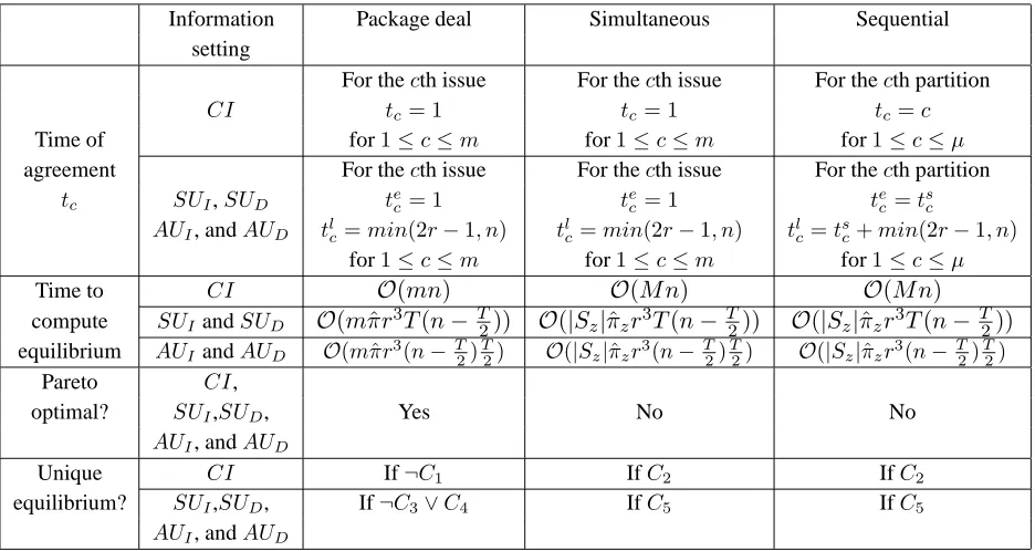
Our methodology is to first derive equilibria for each of the procedures in each of the above settings, From this, we can determine which of them is optimal. As we will see, this analysis shows that, for all the settings, the package deal is the best. We then go on to analyse the procedures in terms of other performance metrics. Specifically, we show that, in all the settings, only the package deal generates a Pareto optimal outcome. We also show that although the package deal may be com-putationally more complex than the other two procedures, it has similar earliest and latest possible times of agreement to the simultaneous procedure (which is better than the sequential procedure), and it (like the other two procedures) generates a unique outcome only in certain situations (which we define). The key results of our study are summarised in Table 1.
Information Package deal Simultaneous Sequential setting
For thecth issue For thecth issue For thecth partition
CI tc= 1 tc = 1 tc=c
Time of for1≤c≤m for1≤c≤m for1≤c≤µ
agreement For thecth issue For thecth issue For thecth partition
tc SUI,SUD t
e
c= 1 t
e
c = 1 t
e c=t
s c
AUI, andAUD tlc=min(2r−1, n) t l
c=min(2r−1, n) t l c =t
s
c+min(2r−1, n) for1≤c≤m for1≤c≤m for1≤c≤µ
Time to CI O(mn) O(M n) O(M n)
compute SUIandSUD O(mπrˆ 3T(n−T2)) O(|Sz|πˆzr3T(n−T2)) O(|Sz|πˆzr3T(n−T2)) equilibrium AUIandAUD O(mπrˆ
3 (n−T
2) T
2) O(|Sz|ˆπzr 3
(n−T 2)
T
2) O(|Sz|πˆzr 3
(n−T 2)
T 2)
Pareto CI,
optimal? SUI,SUD, Yes No No
AUI, andAUD
Unique CI If¬C1 IfC2 IfC2
equilibrium? SUI,SUD, If¬C3∨C4 IfC5 IfC5
[image:4.612.90.558.102.351.2]AUI, andAUD
Table 1: A summary of key results. ts
c denotes the start time for thecth partition, tec the earliest
possible time of agreement, andtl
cthe latest possible time of agreement).
issue case (Sandholm & Vulkan, 1999; Stahl, 1972), and a special type of the sequential procedure for multiple issues (Fatima et al., 2004). See Section 7 for details. Second, it has focussed only on independent issues and asymmetric information settings. Third, it has only focused on finding the optimal procedure, but has not considered the additional solution properties of different procedures. Given this, our paper makes a threefold contribution. First, we obtain the equilibrium for each procedure when there are deadlines. Second, we analyse multiple issues that are both independent and interdependent. Moreover, we analyse both symmetric and asymmetric information settings. Finally, on the basis of the equilibrium for different procedures, we provide the first comprehensive comparison of their solution properties (viz. time complexity, Pareto optimality, uniqueness, and time of agreement). When taken together, the results clearly indicate the choices and tradeoffs involved in choosing a negotiation procedure in a wide range of circumstances. This knowledge can be used by a system designer who is responsible for designing the mechanism that should be used to moderate the negotiation encounters and by the agents themselves if they can choose how to arrange their interactions. Furthermore, this knowledge also tells the agents what their equilibrium offers are during negotiation.
uncer-tainty about the opponent’s utility. In Section 5, we analyse a scenario with asymmetric unceruncer-tainty about the opponent’s utility. Sections 4 and 5 both deal with independent issues. In Section 6, we extend the analysis to interdependent issues. Section 7 discusses the related literature and Section 8 concludes. Appendix A provides a summary of notation employed throughout the paper.
2. Single-Issue Negotiation
Assume there are two agents:aandb. Each agent has time constraints in the form of deadlines and discount factors. Since we focus on competitive scenarios with self-interested agents, we model negotiation using the ‘split the pie game’ analysed by Osborne and Rubinstein (1994), Binmore, Osborne, and Rubinstein (1992). We begin by introducing this complete information game.
Let the two agents be negotiating over a single issue (i). This issue is a ‘pie’ of size 1 and the agents want to determine how to divide it between themselves. There is a deadline (i.e., a number of rounds by which negotiation must end). Let n ∈ N+ denote this deadline. The agents use
Rubinstein’s alternating offers protocol (Osborne & Rubinstein, 1994), which proceeds through a series of time periods. One of the agents, saya, starts negotiation in the first time period (i.e.,t= 1) by making an offer (xi), that lies in the interval [0,1], to b. Agent b can either accept or reject
the offer. If it accepts, negotiation ends in an agreement withagetting a share ofxi andbgetting yi = 1−xi. Otherwise, negotiation proceeds to the next time period, in which agent bmakes a
counter-offer. This process of making offers continues until one of the agents either accepts an offer or quits negotiation (resulting in a conflict). Thus, there are three possible actions an agent can take during any time period: accept the last offer, make a new counter-offer, or quit the negotiation.
An essential feature of negotiations involving alternating offers is that the pie is assumed to shrink with time (Rubinstein, 1982). Specifically, it shrinks at each step of offer and counteroffer. This shrinkage models a decrease in the value of the pie (representing the fact that the pie perishes with time or there is inflation). This shrinkage is represented with a discount factor denoted 0 < δi ≤1for both1agents. Att= 1, the size of the pie is1, but in all subsequent time periodst >1,
the pie shrinks toδit−1.
We denote the set of real numbers byRand the set of real numbers in the interval[0,1]byR1.
Then let[xt
i, yti]denote the offer made at time periodtwherextiandyti denote the share for agenta
andbrespectively. Then, for a given pie, the set of possible offers is:
{[xti, yti] :xti ≥0, yit≥0, and xti+yit=δit−1}
where xt
i ∈ R1 and yti ∈ R1. Each player’s utility function is defined over the set R. Letuai :
R1×N+ →Randubi :R1×N+ →Rdenote the utility functions of the two agents. At timet, if
aandbreceive a share ofxt
i andyitrespectively (wherexit+yit=δt−
1
i ), then their utilities are:
uai(xti, t) =
xt
i ift≤n
0 otherwise
ubi(yti, t) =
yt
i ift≤n
0 otherwise
The conflict utility (i.e., the utility received in the event that no deal is struck) is zero for both agents. Note that δ is not shown explicitly in an agent’s utility function but is implicit. This is because, during any time periodt, xt
i and yti denotea’s andb’s actual shares respectively (not the
ratios of their shares) wherext
i+yit=δt
−1
i . In other wordsδis included in an agent’s share. This
will become clearer when we show the agents’ shares in Expression 1.
For the above setting, the agents reason as follows in order to determine what to offer. Let agent adenote the first mover (i.e., att= 1,aproposes tobhow to split the pie). To begin, consider the case where the deadline for both agents isn= 1. Ifbaccepts, the division occurs as agreed; if not, neither agent gets anything (since n= 1is the deadline). Here,ais in a powerful position and is able to propose to keep 100 percent of the pie and give nothing tob2
. Since the deadline isn= 1, baccepts this offer and agreement takes place in the first time period.
Now, consider the case where the deadline isn= 2. In the first round, the size of the pie is 1 but it shrinks toδi in the second round. In order to decide what to offer in the first round,alooks
ahead tot= 2and reasons backwards3. Agentareasons that if negotiation proceeds to the second round,bwill take 100 percent of the shrunken pie by offering[0, δi]and leave nothing fora. Thus,
in the first time period, ifaoffersbanything less thanδi,bwill reject the offer. Hence, during the
first time period, agentaoffers[1−δi, δi]. Agentbaccepts this and an agreement occurs in the first
time period.
In general, if the deadline isn, negotiation proceeds as follows. As before, agentadecides what to offer in the first round by looking ahead as far as t = nand then reasoning backwards. This decision making leadsato make the following offer in the first time period:
[Σn−1
j=0[(−1)jδ
j
i],1−Σn
−1
j=0[(−1)jδ
j
i]] (1)
Agentbaccepts this offer and negotiation ends in the first time period. Note that the equilibrium outcome depends on who makes the first move. Since we have two agents and either of them could move first, we get two possible equilibrium outcomes.
On the basis of the above equilibrium for single-issue negotiation with complete information, we first obtain the equilibrium for multiple issues and then determine the optimal negotiation procedure for the various settings that we have previously described.
3. Multi-Issue Negotiation with Complete Information
As mentioned in Section 1, the existing literature does not provide an analysis of all the multi-issue procedures for negotiation with deadlines. Hence, we begin by analysing the complete information setting. From this base, we can then extend to the case where there is information uncertainty.
Here aand b negotiate overm > 1 independent issues (Section 6 deals with interdependent issues). These issues aremdistinct pies and the agents want to determine how to split each of them. LetS ={1,2, . . . , m}denote the set ofmpies. As before, each pie is of size 1. Let the discount factor for issue c, where1 ≤ c ≤ m, be0 < δc ≤ 1. For each issue, letndenote each agent’s
2. It is possible thatbmay reject such a proposal. In practice,awill have to propose an offer that is just enough to inducebto accept. However, to keep the exposition simple, we assume thatacan get the whole pie by making the 100 percent proposal.
deadline. In the offer for time periodt(where1≤ t≤n), agent a’s (b’s) share for each of them issues is now represented as anmelement vectorxt ∈Rm
1 (yt∈Rm1 ). Thus, if agenta’s share for
issuecat timetisxt
c, then agentb’s share isyct= (δt−
1
c −xtc). The shares foraandbare together
represented as the package[xt, yt].
We define an agent’s cumulative utility using the additive form. There are two reasons for this. First, it is the most common form for cumulative utilities in traditional multi-issue utility theory (Keeney & Raiffa, 1976). Second, additive cumulative utilities are linear and so the problem of making tradeoffs becomes computationally tractable4. The functionsUa :Rm
1 ×Rm1 ×N +
→ R
andUb :Rm
1 ×Rm1 ×N +
→Rgive the cumulative utilities foraandbrespectively at timet. These
are defined as follows:
Ua([xt, yt], t) =
(
Σm
c=1kcauac(xtc, t) ift≤n
0 otherwise (2)
Ub([xt, yt], t) =
(
Σm
c=1kbcubc(yct, t) ift≤n
0 otherwise (3)
whereka∈Rm
+ denotes anmelement vector of constants for agentaandkb ∈Rm+that forb. Here
R+denotes the set of positive real numbers. These vectors indicate how the agents value different
issues. For example, if ka
c > kac+1, then agent avalues issue cmore than issue c+ 1. Likewise
for agentb. In other words, themissues are perfect substitutes (i.e., all that matters to an agent is its total utility for all themissues and not that for any subset of those Varian, 2003; Mas-Colell, Whinston, & Green, 1995). In all the settings we study, the issues will be perfect substitutes.
Each agent has complete information about all negotiation parameters (i.e.,n,m,ka
c,kcb, andδc
for1 ≤c ≤m). For this complete information setting, we now determine the equilibrium for the package deal, the simultaneous procedure, and the sequential procedure.
3.1 The Package Deal Procedure
In this procedure, the agents use the same protocol as for single-issue negotiation (described in Sec-tion 2). However, an offer for the package deal includes a proposal for each issue under negotiaSec-tion. Thus, formissues, an offer includesmdivisions, one for each issue. Agents are allowed to either accept a complete offer (i.e., allmissues) or reject a complete offer. An agreement can therefore take place either on allmissues or on none of them.
As per single-issue negotiation, an agent decides what to offer by looking ahead and reasoning backwards. However, since an offer for the package deal includes a share for all the m issues, agents can now make tradeoffs across the issues in order to maximise their cumulative utilities. For 1≤c≤m, the equilibrium offer for issuecat timetis denoted as[at
c, btc]whereatc andbtcdenote
the shares for agent aand brespectively. We denote the equilibrium package at timetas[at, bt]
whereat ∈ Rm
1 (bt ∈ Rm1) is an melement vector that denotes a’s (b’s) share for each of the m
issues. Also, for 1 ≤ t ≤ n, δt−1
∈ Rm1 is anmelement vector that represents the sizes of the
mpies at timet. The symbol 0 denotes anmelement vector of zeroes. Note that for1 ≤ t ≤n, at+bt = δt−1 (i.e., the sum of the agents’ shares (at timet) for each pie is equal to the size of
the pie att). Finally, for time periodt(for1 ≤ t ≤ n) we let a(t)(respectively b(t)) denote the equilibrium strategy for agenta(respectively b).
As mentioned in Section 1, the package deal allows agents to make tradeoffs. We letTRADEOFFA
(TRADEOFFB) denote agenta’s (b’s) function for making tradeoffs. Given this, the following
theo-rem characterises the equilibrium for the package deal procedure.
Theorem 1 For the package deal procedure, the following strategies form a Nash equilibrium. The
equilibrium strategy fort=nis:
a(n) =
OFFER [δn−1
,0] IFa’s TURN ACCEPT IFb’s TURN
b(n) =
OFFER [0, δn−1] IFb’s TURN
ACCEPT IFa’s TURN
For all preceding time periodst < n, if[xt, yt]denotes the offer made at timet, then the equilibrium strategies are defined as follows:
a(t) =
OFFER tradeoffa(ka, kb, δ,ub(t), m, t) IFa’s TURN
If (Ua([xt, yt], t)≥ua(t))ACCEPT else REJECT IFb’s TURN
b(t) =
OFFER tradeoffb(ka, kb, δ,ua(t), m, t) IFb’s TURN
If (Ub([xt, yt], t)≥ub(t))ACCEPT else REJECT IFa’s TURN
whereua(t) = Ua([at+1, bt+1], t+ 1)and ub(t) = Ub([at+1, bt+1], t+ 1). An agreement takes
place att= 1.
Proof: We look ahead to the last time period (i.e.,t = n) and then reason backwards. To begin, if negotiation reaches the deadline (n), then the agent whose turn it is takes everything and leaves nothing for its opponent. Hence, we get the strategies a(n)andb(n)as given in the statement of the theorem.
In all the preceding time periods (t < n), the offering agent proposes a package that gives its opponent a cumulative utility equal to what the opponent would get from its own equilibrium offer for the next time period. During time periodt, eitheraorbcould be the offering agent. Consider the case whereamakes an offer att. The package thataoffers attgivesba cumulative utility of Ub([at+1
, bt+1
], t+ 1). However, since there is more than one issue, there is more than one package that givesba cumulative utility ofUb([at+1, bt+1], t+ 1). From among these packages,a
offers the one that maximises its own cumulative utility (because it is a utility maximiser). Thus, the problem forais to find the package[at, bt]so as to:
maximise Σm
c=1kcaatc
such that Σmc=1(δt− 1
c −atc)kcb =ub(t)
This tradeoff problem is similar to the fractional knapsack problem (Martello & Toth, 1990; Cor-men, Leiserson, Rivest, & Stein, 2003), the optimal solution for which can be generated using a greedy approach5 (i.e., by filling the knapsack with items in the decreasing order of value per unit weight). The items in the knapsack problem are analogous to the issues in our case. The only differ-ence is that the fractional knapsack problem starts with an empty knapsack and aims to fill it with items so as to maximise the cumulative value, while an agent’s tradeoff problem can be viewed as starting with the agent having 100 per cent of all the issues and then aiming to give away portions of issues to its opponent so that the latter gets a given cumulative utility, while the resulting loss in its own utility is minimised. Thus, in order to find how to split themissues, agent aconsiders ka
c/kcbfor1≤c≤mbecausekac/kbcis the utility thataneeds to give up in order increaseb’s utility
by one. Sinceawants to maximise its own utility and giveba utility ofUb([at+1
, bt+1
], t+ 1), it divides thempies such that it gets the maximum possible share for those issues for whichka
c/kcbis
high and gives to agentbthe maximum possible share for those issues for whichka
c/kcbis low. Thus, abegins by givingbthe maximum possible share for the issue with the lowestka
c/kbc. It then does
the same for the issue with the next lowestka
c/kbc and repeats this process untilbgets a cumulative
utility ofUb([at+1, bt+1], t+ 1). In order to facilitate this process of making tradeoffs, the
individ-ual elements ofkb are arranged such thatka
c/kcb > kca+1/kcb+1. The functiontradeoffatakes six
parameters: ka,kb,δ, ub(t), m, and t and uses the above described greedy method to solve the
maximisation problem given in Equation 4 and return the corresponding package. If there is more than one package that solves Equation 4, thentradeoffareturns any one of them (because agent
agets equal utility from all such packages and so does agent b). The function tradeoffbfor agentbis analogous to that fora.
On the other hand, the equilibrium strategy for the agent that receives an offer is as follows. For time periodt, letbdenote the receiving agent. Then,baccepts[xt, yt]ifub(t)≤Ub([xt, yt], t),
oth-erwise it rejects the offer because it can get a higher utility in the next time period. The equilibrium strategy foraas receiving agent is defined analogously. Hence we get the equilibrium strategies (a(t)andb(t)) given in the statement of the theorem.
In this way, we reason backwards and obtain the offers fort = 1. The first mover makes this offer and the other agent accepts it. An agreement therefore occurs in the first time period.
Theorem 2 For the package deal procedure, the time taken to determine an equilibrium offer for
t= 1isO(mn)wheremis the number of issues andnis the deadline.
Proof: We know from Theorem 1 that the time to compute the equilibrium offer fort=nis linear in the number of issues (see strategiesa(n)andb(n)). Consider a time periodt < n. During this time period, the functiontradeoffais used to make tradeoffs. The time complexity oftradeoffa (which uses the greedy approach described in the proof of Theorem 1) isO(m)(Martello & Toth, 1990; Cormen et al., 2003). This function needs to be repeated for every time period from the (n−1)th to the first. Hence the time complexity of finding an offer for the first time period is
O(mn).
5. The time complexity of this approach isO(m)(Martello & Toth, 1990), wheremdenotes the number of items. Note that the greedy method for the fractional knapsack problem takesO(m)time regardless of whether the coefficients ka
c andkbc(for1≤c≤m) in Equation 4 are positive or negative (Martello & Toth, 1990). In the present setting
Theorem 3 The package deal procedure generates a Pareto optimal outcome.
Proof: Recall that we consider competitive negotiations. Hence, for an individual issuec (where 1 ≤ c ≤m), an increase in one agent’s utility results in a decrease in that of the other. However, for the package deal procedure, an agent considers its cumulative utility from allm issues. Con-sequently, during the process of backward reasoning, at timet < n, the agent that makes tradeoffs maximises its own cumulative utility without lowering that of its opponent (with respect to what the opponent would offer in the next time period). Hence the equilibrium outcome for the package deal is Pareto optimal.
Theorem 4 For a given first mover, the package deal procedure has a unique equilibrium outcome
if the following condition is false:
C1. There exists ani and a j (where 1 ≤ i ≤ m and 1 ≤ j ≤ m) such that (i 6= j) and
(ka
i/kib =kaj/kjb).
Proof: Consider a time periodt < nand letadenote the offering agent. Recall from Theorem 1 that asplits themissues in the increasing order ofka
i/kbi. Thus, for a giveniandj, ifkia/kbi =kja/kjb,
then agentais indifferent between which of the two issues (iorj) it splits up first. For example, if m = 2,n = 2,δ = 0.5,ka
1 = 1,k2a = 2,k1b = 2, andk2b = 4, thenka1/k1b = k2a/kb2 = 0.5. Ifa
is the offering agent att= 1, it can offer(1,0)for issue 1 and(1/4,3/4)for issue 2. This gives a cumulative utility of 1.5 toaand 3 tob. Alternativelyacan offer(0,1)for issue 1 and(3/4,1/4) for issue 2 since this also results in the same cumulative utilities toaandb.
On the other hand, ifka
i/kib6=kja/kbj, thenasplits issueifirst ifkia/kbi < kaj/kjband issuejfirst
ifka
i/kbi > kja/kjb. In other words, there is only one possible equilibrium offer thatacan make at
any timet < n. Likewise there is one possible equilibrium offer thatbcan make at any timet < n. Since there is a unique offer for each time period, the equilibrium outcome is unique.
Note that the uniqueness we refer to in Theorem 4 is with respect to a given first mover. If the first mover changes, then the equilibrium outcome may change, as the following example illustrates. Letm = 2,n = 2, δ = 0.5,ka
1 = 1, k2a = 2,kb1 = 2, andkb2 = 1. Ifais the offering agent at
t= 1, its equilibrium offer is(1/4,3/4)for the first issue and(1,0)for the second. This results in a cumulative of2.25toaand1.5tob. In contrast, ifbis the offering agent att= 1, its equilibrium offer is(0,1) for the first issue and(3/4,1/4) for the second. This results in a cumulative utility of1.5toaand 2.25tob. In the following discussion, we use the term unique to mean unique with respect to a given first mover.
3.2 The Simultaneous Procedure
For this procedure, them issues are partitioned intoµ > 1disjoint subsets. For 1 ≤ c ≤ µ, let Sc denote thecth partition where∪µc=1Sc ={1, . . . , m}. The issues within each subset are settled
using the package deal. Negotiation for each of theµpartitions starts att= 1. Thus, forµ=m, all missues are settled simultaneously and independently of each other. At the other extreme, we have only one partition (i.e.,µ= 1) which is the package deal procedure described in Section 3.1. Since the issues in each subset (i.e., eachSc) are settled using the package deal, the equilibrium for each
occurs att= 1. Hence, for the simultaneous procedure, an agreement for each partition (and hence each issue) occurs in the first time period.
Second, for the simultaneous procedure, the time taken to determine an equilibrium offer for t= 1isΣµc=1O(|Sc|n)where|Sc|is the number of issues in thecth partition andnis the deadline.
This is explained as follows. Since the time taken to find the equilibrium offer fort = 1for the package deal (i.e., forµ= 1) isO(mn)(see Theorem 2), the time taken to compute the equilibrium offer for t = 1 for the cth partition isO(|Sc|n). Hence, for all µpartitions, the time complexity
isΣµc=1O(|Sc|n)which is equal toO(M n), whereM denotes the number of issues in the largest
partition.
Third, it follows from Theorem 4 that the simultaneous procedure has a unique equilibrium outcome if the following conditionC2is true:
C2. There is no partitionc(where1≤c≤µ) for which the conditionC1is true.
Finally, as Theorem 5 shows, the simultaneous procedure may not generate a Pareto optimal outcome.
Theorem 5 The simultaneous procedure may not generate a Pareto optimal outcome.
Proof: The package deal allows tradeoffs to be made across all themissues, while the simultaneous procedure allows tradeoffs to be made across issues within each partition but not across partitions. Hence the simultaneous procedure may not generate a Pareto optimal outcome. We show this with a counter example. Consider the case wheren= 2,δ= 0.5,m = 3,µ= 2,S1 ={1,2},S2 ={3},
ka
1 = 1,ka2 = 2,ka3 = 3,k1b = 1,kb2 = 0.5, andkb3 = 0.25. Letadenote the first mover. From
Theorem 1, we know that in the equilibrium for partitionS1, agentagets a share of0.25for issue
1and1for issue2, andbgets a share of0.75for issue1and nothing for issue2. For partition S2,
each agent gets a share of1/2. Thus,a’s cumulative utility from all three issues is3.75and that of bis0.875.
Now consider the case where all three issues are discussed using the package deal. Here,µ= 1 and all other parameters remain the same. In the equilibrium outcome for this procedure,agets a cumulative utility of5.125 and bgets0.875. This means that the procedure with µ = 2does not generate a Pareto optimal outcome.
3.3 The Sequential Procedure
For this procedure, themissues are partitioned intoµ >1disjoint subsets. For1 ≤c≤µ, letSc
denote thecth partition where∪µc=1Sc ={1, . . . , m}. Theµpartitions are negotiated sequentially,
one after another. The issues within a subset are settled using the package deal. Negotiation for the first partition starts at timet = 1. If negotiation for thecth (for1 ≤ c ≤ µ) partition ends attc,
then negotiation for the(c+ 1)th partition starts at timetc+ 1. Each player gets its share for all
the issues in a partition as soon as the partition is settled. Thus, forµ=m, allmissues are settled in sequence. At the other extreme, we have only one partition (i.e., µ = 1) which is the package deal procedure described in Section 3.1. Since the issues in each subset (i.e., each Sc) are settled
Theorem 6 For the sequential procedure, the equilibrium time of agreement for the cth partition (for1≤c≤µ) isTc =c.
Proof: From Theorem 1, we know that an agreement for the package deal occurs in the first time period. Hence, negotiation for each partition ends in the same time period in which it starts (i.e., negotiation for thecth partition starts att=cand results in an agreement in the same time period). The time taken to settle all themissues is thereforeµ.
Note that the time complexity of the sequential procedure (i.e., the time to compute equilibrium offers) is the same as that for the simultaneous procedure. Also, like the simultaneous procedure, the equilibrium outcome for the sequential procedure may not be Pareto optimal. Finally, the condition for the equilibrium outcome for the sequential procedure to be unique is the same as that for the simultaneous procedure.
3.4 The Optimal Procedure
Having obtained the equilibrium outcomes for the three multi-issue procedures, we now compare them in terms of the utilities they generate for each player. Then the procedure that gives a player the maximum utility is its optimal one.
Note that, for the sequential procedure, the equilibrium outcome strongly depends on the order in which the partitions are settled. This ordering is called the negotiation agenda. There are two ways of defining the agenda (Fershtman, 1990): exogenously or endogenously. If the agenda is determined before the actual negotiation over the issues begins, then it is said to be exogenous. On the other hand, for the endogenous agenda, the agents decide what issue they will settle next during the process of negotiation. The agenda that gives an agent the maximum utility between all possible agendas is its optimal one (Fatima et al., 2004). Our objective here is not to determine the optimal agenda, but to consider a given agenda and compare the equilibrium outcome for the sequential procedure for that agenda with the outcomes for the simultaneous and the package deal procedures, in order to find the optimal procedure. The following theorem characterises this procedure.
Theorem 7 Irrespective of how them issues are split intoµ > 1partitions, the package deal is optimal for both parties.
Proof: In order to compare an agent’s utility from different procedures, it is important to take into account who initiates negotiation. For the package deal, the first mover makes an offer on all the issues. Hence we compare an agent’s utilities for the three procedures, given the agent that will be the first mover for all the three procedures for all the issues.
We first show that the outcome for the package deal is no worse than that for the simultaneous procedure. Consider the simultaneous procedure for anyµ >1. For this procedure, fort≤n, the offering agent makes tradeoffs across the issues in each partition independently of the other parti-tions. Now consider the package deal procedure (i.e., withµ = 1partitions). For this procedure, the offering agent makes tradeoffs across allmissues. Since the difference between the procedure withµ= 1and the one withµ >1is that the former makes tradeoffs across allmissues while the latter does not, each agent’s utility from the former procedure is no worse than its utility from the latter.
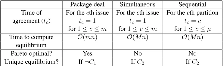
Package deal Simultaneous Sequential Time of For thecth issue For thecth issue For thecth partition
agreement (tc) tc = 1 tc = 1 tc=c
for1≤c≤m for1≤c≤m for1≤c≤µ
Time to compute O(mn) O(M n) O(M n)
equilibrium
Pareto optimal? Yes No No
[image:13.612.121.493.102.213.2]Unique equilibrium? If¬C1 IfC2 IfC2
Table 2: A comparison of the outcomes for the three multi-issue procedures for the complete infor-mation setting (CI).
• Partitionc = 1. Since negotiation for the first partition starts att = 1for both the simulta-neous and the sequential procedures, the outcome for this partition is the same forµ= 1and µ >1. Hence, for the first partition, an agent gets equal utility from the two procedures.
• Partition c > 1. Let agent adenote the first mover for partition c (for 2 ≤ c ≤ µ) for both simultaneous and sequential procedures. Also, letUa
simandUseqa denotea’s cumulative
utility for this partition from the equilibrium outcome for the simultaneous and the sequential procedures respectively. Likewise, let Ub
sim and Useqb denote b’s cumulative utility for this
partition from the equilibrium outcome for the simultaneous and the sequential procedures respectively.
Now for the simultaneous procedure, negotiation for each partition starts in the first time period. An agreement for each partition also occurs in the first time period. On the other hand, for the sequential procedure, negotiation for thecth partition starts in thecth time period and results in an agreement in the same time period (see Theorem 6). Since each pie shrinks with time, agenta’s cumulative utility Ua
sim is greater thanUseqa , and agentb’s cumulative utility Ub
simis greater thanUseqb .
Thus, the simultaneous procedure is better than the sequential one for both agents. Furthermore (as shown above), the outcome for the package deal is no worse than that for the simultaneous procedure for both agents. Therefore, for each agent, the package deal is the optimal procedure.
These results are summarised in Table 2. For the above analysis, the negotiation parametersn,δc, ka
c, andkbc (for1 ≤ c ≤ m) were common knowledge to the agents. However, this is unlikely to
be the case for most encounters. Therefore we now extend this analysis to incomplete information scenarios with uncertainty about utility functions6. In Section 4, we focus on the symmetric infor-mation setting where each agent is uncertain about the other’s utility function. Then, in Section 5, we examine the asymmetric information setting where one of the two agents is uncertain about the other’s utility function, but the other agent knows the utility function of both agents.
4. Multi-Issue Negotiation with Symmetric Uncertainty about the Opponent’s Utility
In this symmetric information setting, each agent is uncertain about its opponent’s utility function: for1≤c≤m, agenta(b) is uncertain aboutkb
c(kca). Specifically, letKdenote a vector ofrvectors
where each vectorKi ∈ Rm+ (for 1≤ i≤r) consists ofmconstant positive real numbers. These
r vectors are the possible values forka ∈ Rm
+ and kb ∈ Rm+. In other words, there are r types 7
for agentaandrtypes for agentb. LetPa:N+
→ R1denote the discrete probability distribution
function forkaandPb:N+
→R1that forkb. The domain for these two functions is[1..r]. In other
words, for1≤i≤r,Pa(i)(Pb(i)) is the probability that agenta(b) is of typei. For1≤c≤m,
letKicdenote thecth element of vectorKi.
In this setting, the vector Kand the functionsPaandPbare common knowledge to the
nego-tiators. Also, each agent knows its own type, but not that of its opponent. In addition, each agent knowsr,δ,n, andm.
Since there are r types for agent aand r types for agentb, we define r different cumulative utility functions for each of the two agents. If agenta(b) is of typei(for1≤i≤r) then its utility Ua
i :Rm1 ×Rm1 ×N +
→R(Ub
i :Rm1 ×Rm1 ×N +
→R) from the division specified by the package
[xt, yt]at timetis:
Uia([xt, yt], t) =
(
Σm
c=1Kicuac(xtc, t) ift≤n
0 otherwise (5)
Uib([xt, yt], t) =
(
Σm
c=1Kicubc(yct, t) ift≤n
0 otherwise (6)
Note that, as before, the issues are perfect substitutes. For this setting, we determine the equi-librium outcomes for each of the three multi-issue procedures and then compare them.
4.1 The Package Deal Procedure
We know from Theorem 1 that the equilibrium outcome for the complete information setting de-pends on ka
c and kcb (for 1 ≤ c ≤ m). However, in this setting, there is uncertainty aboutkcaand kb
c. Hence we use the standard expected utility theory (Neumann & Morgenstern, 1947; Fishburn,
1988; Harsanyi & Selten, 1972) to find an agent’s optimal strategy. Before doing so, however, we first introduce some notation.
For1 ≤ i ≤ r, we leta(i, t) denote the equilibrium strategy for an agentaof typeifor the time periodt. Analogously,b(i, t)denotes the equilibrium strategy for an agentbof typeifor the time periodt. Note that for1 ≤ i ≤ r, if [at, bt]is the package offered at timetin equilibrium,
thenat+bt =δt−1
(i.e., for each pie, the sum of the shares of the two agents is equal to the size of the pie at timet). Also, for1 ≤ i ≤ r, we leta(i, j, t) denote the equilibrium strategy for an agentaof typeifor the time periodt, assuming thatbis of typej. Analogously,b(i, j, t)denotes the equilibrium strategy for an agentbof typeifor the time periodt, assuming thatais of typej.
Also, leteua(i, t)denote the cumulative utility that an agentaof typeiexpects to get fromb’s equilibrium offer at timet(i.e., ais the receiving agent andb the offering agent att). Likewise, eub(i, t)denotes the cumulative utility that an agentbof typeiexpects to get froma’s equilibrium offer at timet(i.e.,bis the receiving agent andathe offering agent att). We leteua(i, j, t)denote agent a’s expected cumulative utility from its own equilibrium offer at time t if a is of type i,
assuming thatbis of typej. Note that this isa’s utility when it is the offering agent att. And let eub(i, j, t)denote agentb’s expected cumulative utility from its own equilibrium offer at timetifb is of typeiand assuming thatais of typej. Note that this isb’s utility when it is the offering agent att.
Recall that in this setting, each agent only knows its own type, but not that of its opponent. Since there arer possible types, there are r possible offers an agent can make at any time period (one offer corresponding to each of the opponent’s types). Among theseroffers, the one that gives an agent the maximum expected cumulative utility is its optimal offer. If thecth offer (1 ≤c ≤r) gives an agent the maximum expected cumulative utility, then we say that the optimal choice for the agent isc. For time periodt, we letopta(i, t)(optb(i, t)) denote the optimal choice for agenta (b) of typei.
Att=n, the offering agent gets everything and the opponent gets zero utility. Thus, fort=n, we have the following:
eua(i, n) = 0 for1≤i≤r (7)
eub(i, n) = 0 for1≤i≤r (8)
eua(i, j, n) =
m
X
c=1
Kicδct−1 for1≤i≤rand1≤j≤r (9)
eub(i, j, n) =
m
X
c=1
Kicδct−1 for1≤i≤rand1≤j≤r (10)
Note that fort=n,eua(i, j, n)andeub(i, j, n)do not depend onjbecause in the last time period, the offering agent gets 100 percent of all thempies. For all preceding time periodst < n, we have the following:
eua(i, t) = eua(i, θ, t+ 1) for1≤i≤rwhereθ=opta(i, t+ 1) (11)
eub(i, t) = eub(i, λ, t+ 1) for1≤i≤rwhereλ=optb(i, t+ 1) (12)
eua(i, j, t) =
r
X
e=1
Fa(i, j, e, t)×Pb(e) for1≤i≤rand1≤j≤r (13)
eub(i, j, t) =
r
X
e=1
Fb(i, j, e, t)×Pa(e) for1≤i≤rand1≤j≤r (14)
The functionFatakes four parameters: i,j,e, andt, and returns the utility that an agentaof type igets from offering the equilibrium package for timet, assuming that agentbis of typejwhere in fact it is of typee. Obviously, agentbacceptsa’s offer attifUb
e(a(i, j, t), t) ≥ eub(e, γ, t+ 1)
whereγ =optb(e, t+ 1). Otherwise, agentbrejectsa’s offer and negotiation proceeds to the next round in which casea’s expected utility isEUA(i, t+ 1). Hence,Fais defined as follows:
Fa(i, j, e, t) =
Ua
i(a(i, j, t), t) if Ueb(a(i, j, t), t) ≥eub(e, γ, t+ 1)whereγ =optb(e, t+ 1)
eua(i, t+ 1) otherwise
where the strategya(i, j, t)fort=nis defined as follows:
A(i, j, n) =
OFFER[δn−1
,0] ifa’s turn
and for all preceding time periodst < nit is defined as:
A(i, j, t) =
OFFERtradeoffa1(K, δ,eub(j, t), i, j, m, t, Pa, Pb) ifa’s turn ifUa
i([xt, yt], t)≥EUA(i, t)ACCEPT else REJECT otherwise
where [xt, yt]denotes the offer made at t and the function8
TRADEOFFA1 is defined as follows. LikeTRADEOFFA, the functionTRADEOFFA1 solves the following maximisation problem:
maximise Σmc=1Kicatc
such that Σm c=1(δt
−1
c −atc)Kjc=eub(j, t)
0≤at
c ≤1 for1≤c≤m (15)
where i denotes a’s type and j that of b. However, the difference between TRADEOFFA1 and
TRADEOFFAarises when there is more than one package that maximisesa’s cumulative utility (i.e.,
Σm
c=1Kicatc) while givingba cumulative utility ofeub(j, t). If there is more than one such package,
then in Theorem 1, it does not matter which of these packages aoffers tob(because both agents have complete information). Hence, TRADEOFFA can return any one such package. However, in the present setting, there is uncertainty. Therefore, if there is more than one package that maximises a’s cumulative utility while givingba cumulative utility ofeub(j, t), then TRADEOFFA1 returns the package that maximises a’s expected cumulative utility. For instance, let[at, bt]be one such
package that maximises a’s cumulative utility. Thena’s expected cumulative utility from[at, bt]
(i.e.,eua(i, j, t)) is as given in Equation 13 where:
Fa(i, j, e, t) =
Ua
i([at, bt], t) if Ueb([at, bt], t)≥eub(e, γ, t+ 1)whereγ =optb(e, t+ 1)
eua(i, t+ 1) otherwise
Obviously, if there is more than one package that maximises a’s expected cumulative utility and givesba utility ofeub(j, t)thenTRADEOFFA1 returns any one such package.
We now turn to agentb. For this agent,Fb,B(i, j, t), andtradeoffb1are defined analogously
as follows:
Fb(i, j, e, t) =
Ub
i(b(i, j, t), t) if Uea(b(i, j, t), t)≥eua(e, α, t+ 1)whereα =opta(e, t+ 1)
eub(i, t+ 1) otherwise
where the strategyb(i, j, t)fort=nis defined as follows:
B(i, j, n) =
OFFER[0, δn−1
] ifb’s turn
ACCEPT otherwise
and for all preceding time periodst < nit is defined as:
B(i, j, t) =
OFFERtradeoffb1(K, δ,eua(j, t), i, j, m, t, Pa, Pb) ifb’s turn ifUb
i([xt, yt], t)≥EUB(i, t)ACCEPT else REJECT otherwise
Thus, the optimal choice for agenta(i.e.,opta(i, t)) and that for agentb(i.e.,optb(i, t)) are defined as follows:
opta(i, t) = arg maxr
j=1eua(i, j, t) for1≤i≤r (16)
optb(i, t) = arg maxrj=1eub(i, j, t) for1≤i≤r (17)
Note that the offering agent’s optimal choice fort=ndoes not depend on its opponent’s type since the offering agent gets all the pies.
We compute the optimal choice for the first time period by reasoning backwards from t = n. Att= 1, if an agentaof typeiis the offering agent, then it offers the package that corresponds to agentbbeing of typeopta(i,1). Likewise, if an agentbof typeiis the offering agent, then it offers the package that corresponds to agentabeing of typeoptb(i,1).
However, sinceopta(i,1)andoptb(i,1)are obtained in the absence of complete information, an agreement may or may not take place in the first time period. If an agreement does not occur att = 1, then the agents need to update their beliefs as follows. LetTa
t ⊆ {1,2, . . . , r}denote
the set of possible types for agentaat timet. Fort = 1, we haveTa
1 = {1,2, . . . , r}and T1b = {1,2, . . . , r}. Assume that an agentaof typeimakes an offer att = 1. If the offer thatamakes gets rejected, then it means thatbis not of typeopta(i,1)and soaupdates its beliefs aboutbusing Bayes’ rule. Now, on the basis ofa’s offer att = 1(say [x1
, y1
]), agent bcan infer the possible types for agenta. Thus, agentbtoo updates its beliefs using Bayes’ rule. The belief update rules for timetare as defined below.
UPDATE BELIEFS: Agentaputs all the weight of the posterior distribution ofb’s type overTb
t − {optb(i, t)}using Bayes’ rule. Agentbputs all the weight of the posterior
distribution ofa’s type overKusing Bayes’ rule whereK ⊆ {1,2, . . . , r}is the set of possible types forathat can offer[xt, yt]in equilibrium.
The belief update rule for the case whereboffers att = 1is analogous to the above case wherea offers att= 1.
Thus if the offer att = 1gets rejected, then negotiation goes to the next round. Att= 2, the offering agent (say an agentaof typei) findsopta(i,2)with its updated beliefs. This process of updating beliefs and making offers continues until an agreement is reached.
In Section 3, we used the concept of Nash equilibrium because the agents had complete infor-mation. However, in the current setting, each agent is uncertain about its opponent’s type and so an agent’s optimal strategy depends on its beliefs about its opponent. Hence we use the concept of sequential equilibrium (Kreps & Wilson, 1982; van Damme, 1983) for this setting. Sequential equilibrium is defined in terms of two elements: a strategy profile and a system of beliefs. The strategy profile comprises of a pair of strategies, one for each agent. The belief system has the fol-lowing properties. Each agent has a belief about its opponent’s type. In each time period, an agent’s strategy is optimal given its current beliefs (during the time period) and the opponent’s possible strategies. For each time period, each agent’s beliefs (about its opponent) are consistent with the offers it received. Using this concept of sequential equilibrium, the following theorem characterises the equilibrium for the package deal procedure.
Theorem 8 For the package deal procedure, the following strategies form a sequential equilibrium.
The equilibrium strategies fort=nare:
a(i, n) =
OFFER [δn−1
b(i, n) =
OFFER [0, δn−1
] IFb’s TURN ACCEPT IFa’s TURN
for1≤i≤r. For all preceding time periodst < n, if[xt, yt]denotes the offer made at timet, then the equilibrium strategies are defined as follows:
a(i, t) =
OFFER tradeoffa1(K, δ,eub(ψ, t), i, ψ, m, t, Pa, Pb) IFa’s TURN
If offer gets rejected UPDATE BELIEFS
RECEIVE OFFER and UPDATE BELIEFS IFb’s TURN If (Ua
i ([xt, yt], t)≥eua(i, t))ACCEPT else REJECT
b(i, t) =
OFFER tradeoffb1(K, δ,eua(φ, t), i, φ, m, t, Pa, Pb) IFb’s TURN
If offer gets rejected UPDATE BELIEFS
RECEIVE OFFER and UPDATE BELIEFS IFa’s TURN If (Ub
i(xt, yt], t)≥eub(i, t))ACCEPT else REJECT
for1 ≤i≤r. Here,ψ=opta(i, t)andφ=optb(i, t). The earliest possible time of agreement
ist= 1and the latest possible time of agreement ist=min(2r−1, n).
Proof: At timet = n, the offering agent takes all the pies and leaves nothing for its opponent. The opponent accepts this and we get a(i, n) and b(i, n). Now consider a time period t < n. Recall that during negotiation for the complete information setting (see Section 3.1), at timet < n, the offering agent proposes a package that gives its opponent a cumulative utility equal to what the opponent would get from its own equilibrium offer for the next time period. However, for the current incomplete information setting, an agent knows its own type but not that of its opponent. Hence, for this scenario, at timet < n, the offering agent (say a) proposes a package that givesb an expected cumulative utility equal to whatbwould get from its own equilibrium offer for the next time period (i.e.,eub(ψ, t)). This package is determined by thetradeoffa1function. Likewise, if b is the offering agent at time t, then it makes tradeoffs using tradeoffb1 and offers a an expected cumulative utilityeua(φ, t).
We obtain the equilibrium offer fort = n−1and then reason backwards until we obtain the equilibrium offer fort = 1. However, since these offers are computed in the absence of complete information (i.e., on the basis of expected utilities), an agreement may or may not take place at t= 1. If an agreement does not take place att= 1, then negotiation proceeds as follows. Consider a time period t such that 1 ≤ t < n. Let [xt, yt] denote the offer made at time t. The agent
that receives the offer (say agenta) updates its beliefs using Bayes’ rule: put all the weight of the posterior distribution ofb’s type overKwhereK ⊆ {1,2, . . . , r}is the set of possible types forb that can offer[xt, yt]in equilibrium. If the proposed offer ([xt, yt]) gets rejected, then the offering
agent (say agentbof typei) updates its beliefs using Bayes’ rule: put all the weight of the posterior distribution ofa’s type overTa
t − {optb(i, t)}. The belief update rule for the case where agenta
offers at timetare analogous to the above rule. These belief update rules when incorporated in the agents’ strategies givea(i, t)andb(i, t)as shown in the statement of the theorem.
The earliest possible time of agreement ist= 1. We show this with the following example. Let n= 2,m= 2,r= 2,δ= 1/2, andK = [1,2; 5,1]. Let agentabe the offering agent at timet= 1. Assume thatais of type 1 (i.e.,ka= [1,2]). LetPb(1) = 0.1andPb(2) = 0.9. Sincer= 2, agent acan play two possible strategies at timet= 1: one that corresponds to the case wherebis of type 1 and the other that corresponds to the case wherebis of type 2. For the former case,a’s equilibrium offer att = 1is[0,1]for the first issue and[3
4, 1
4]for the second one. Henceeua(1,1,1) = 1.5.
For the latter case,a’s equilibrium offer att= 1is[2 5,
3
5]for the first issue and[1,0]for the second
issue. Henceeua(1,2,1) = 2.16. Sinceeua(1,2,1) >eua(1,1,1),opta(1,1) = 2andaplays the latter strategy. Now ifbis in fact of type 2, then it acceptsa’s offer att= 1. But ifbis in fact of type 1, it rejectsa’s offer att= 1since it can get a higher utility att= 2. An agreement therefore occurs att= 2. Thus, the earliest possible time of agreement ist= 1.
Now consider the case where anaof typeioffers att= 1but an agreement does not occur at this time. Whena’s offer gets rejected, it knows thatbis not of typeopta(i,1). Thus the number of possible types forbis now reduced tor−1. This happens every timeamakes an offer (i.e., every alternate time period) but it gets rejected. When negotiation reaches time periodt= 2r−1, there is only one possible type forb. Likewise, there is only one possible type for agenta. An agreement therefore takes place att= 2r−1. However, ifn <2r−1then an agreement occurs att=n(see a(i, n)andb(i, n)). In other words, if an agreement does not occur at t= 1, then it occurs at the latest byt=min(2r−1, n).
As we mentioned earlier, if there is more than one package that solves Equation 15, thentradeoffa1 returns the one that maximisesa’s expected cumulative utility. Letpaij
t (whereidenotesa’s type
andjthat ofb) denote the set of all possible packages thattradeoffa1can return at timet. The setpbij
t for agentbis defined analogously.
Theorem 9 For a given first mover, the package deal procedure has a unique equilibrium outcome
if the conditionC3is false orC4 is true.
C3. There exists ani,j,c, andd, such that (c6=d) and (i=6 j) and (Kic/Kjc=Kid/Kjd) where
1≤i≤r,1≤j ≤r,1≤c≤m, and1≤d≤m.
C4. |paijt|= 1and|pbijt |= 1where1≤i≤r,1≤j≤r,i6=j, and1≤t≤n.
Proof: Letidenote agenta’s type andjdenote b’s type wherei6=j,1 ≤i≤r, and1≤ k≤r. Note that ifaandbare of the same type, they have similar preferences for different issues. Soi6=j because the agents gain from making tradeoffs when they are of different types. The rest of the proof for the conditionC3follows from Theorem 4. ConsiderC4. IfC3is true, then we know that,
at timet,tradeoffa1returns that package that solves Equation 15 and maximisesa’s expected cumulative utility. Hence ifpaij
t contains a single element, then there is only one possible package
that tradeoffa1can return. Likewise, ifpbij
t contains a single element, then there is only one
possible package that tradeoffb1can return. If there is only one possible offer for each time period1≤t≤n, then the equilibrium outcome is unique.
know from Theorem 1 that using the greedy approach,tradeoffaconsiders the missues in the increasing order ofKic/Kjc whereidenotesa’s type andjdenotesb’s type. LetSpij ⊆Sdenote a
set of issues (where0 ≤Dij < m,1≤p ≤Dij,idenotesa’s type, andj denotesb’s type) such
that:
|Spij|>1 for1≤p≤Dij
and:
∀c,d∈Sij p
Kic Kjc
= Kid Kjd
In other words,Spijis a set of issues such that ifcanddbelong toSpijthenKic/Kjc =Kid/Kjd, and Dij is the number of sets that satisfy this condition. So ifDij = 0then it means that there is only
one package that solves Equation 15. But ifDij >0then there is more than one package that solves
Equation 15 and from among these tradeoffa1must find the one that maximisesa’s expected cumulative utility. For example if the set of issues isS = {1,2,3,4}, r = 2,K1 = {5,6,7,8},
andK2 ={9,6,7,8}, thenD12 = 1,S112 ={2,3,4}, and|S 12
1 |= 3. So while making tradeoffs,
acan consider the issues inS12
1 in any order because for all the three issues it needs to give up the
same amount of utility in order to increaseb’s utility by 1. The three issues inS12
1 can be ordered
in3! different ways resulting in 3! different packages. From among these 3!different packages, tradeoffa1must find the one that maximises a’s expected cumulative utility. In general, for
Dij >1, letπij denote the number9
of possible packagestradeoffa1needs to consider where
πij is:
πij = Dij Y
p=1 |Sij
p |!
In other words, ifa’s type isiandb’s type isj, then there areπij packages that solve Equation 15
and from among these tradeoffa1must find the one that maximises a’s expected cumulative utility. So ifDij = 0, thenπij = 1. Letπˆbe defined as:
ˆ
π = max
1≤i≤r,1≤j≤r,i6=jπ
ij (18)
In other words, πˆ is the maximum number of packages thattradeoffa1will have to search to find the one that maximises a’s expected cumulative utility (considering all possible types of a and all possible types of b). Note that, as before, a and b are of different types (i.e., i 6= j in Equation 18) because the agents gain from making tradeoffs when they are of different types. The time complexity oftradeoffa1depends onπˆ.
Theorem 10 The time complexity oftradeoffa1isO(mπˆ).
Proof: We know from Theorem 2 that the time complexity of finding any one package that solves Equation 15 is O(m). However, if there is more than one package that solves Equation 15 then tradeoffa1returns the one that maximisesa’s expected cumulative utility. The time to compute
a’s expected cumulative utility from any one such package isO(m). The maximum number of such packages for whichaneeds to find its expected cumulative utility isπˆ. Thus the time complexity of tradeoffa1isO(mπˆ).
9. Note thatπij
is defined in terms of the factorial of|Sij
p|, but|Spij|is independent of mand it is assumed that |Sij