Application of Analog Adaptive Filters
for Dynamic Sensor Compensation
Mehdi Jafaripanah, Bashir M. Al-Hashimi
, Senior Member, IEEE
, and Neil M. White
, Senior Member, IEEE
Abstract—This paper investigates the application of analog adaptive techniques to the area of dynamic sensor compensation, of which there is little reported work in the literature. The case is illustrated by showing how the response of a load cell can be improved to speed up the process of measurement. The load cell is a sensor with an oscillatory response in which the measurand contributes to the response parameters. Thus, a compensation filter needs to track variation in measurand, whereas a simple fixed filter is only valid at one specific load value. To facilitate this investigation, computer models for the load cell and the adaptive compensation filter have been developed. To allow a practical implementation of the adaptive techniques, a novel piecewise linearization technique is proposed in order to vary a floating voltage-controlled resistor in a linear manner over a wide range. Simulation and practical results are presented, thus, demonstrating the effectiveness of the proposed techniques.
Index Terms—Analog adaptive filter, dynamic sensor, load cell, response compensation.
I. INTRODUCTION
L
OAD CELLS are used in a variety of industrial weighing applications such as vending machines and check-weighing systems. Since information processing and control systems cannot function correctly if they receive inaccurate input data, compensation of the imperfections of sensors is one of the most important aspects of sensor research. Influence of unwanted signals, nonideal frequency response, parameter drift, nonlinearity, and cross sensitivity are the five major defects in primary sensors [1]. In the new generation of sen-sors, called intelligent or smart sensen-sors, the influence of these imperfections has been dramatically reduced by using signal processing techniques, which have resulted from advances in the field of digital systems.Some sensors, such as load cells, have an oscillatory response which needs time to settle down. Dynamic measurement refers to the ascertainment of the final value of a sensor signal while its output is still in oscillation. It is, therefore, necessary to deter-mine the value of the measurand in the fastest time possible to speed up the process of measurement, which is of particular im-portance in some applications including vending machines and checkweighing systems. One example of processing that can be done on the sensor output signal is filtering to achieve response correction. Several methods have been reported addressing this
Manuscript received February 25, 2003; revised May 21, 2004. An earlier version of this paper was presented at the IEEE International Symposium on Circuits and Systems, Bangkok, Thailand, May 25–28, 2003
The authors are with the School of Electronics and Computer Sci-ence, University of Southampton, Southampton SO17 1BJ, U.K. (e-mail: [email protected]; [email protected]; [email protected]).
[image:1.594.304.552.162.308.2]Digital Object Identifier 10.1109/TIM.2004.839763
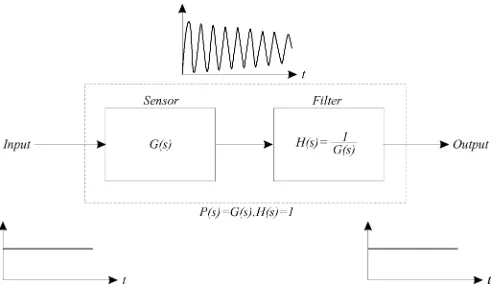
Fig. 1. General principle of load cell response correction.
problem. Software techniques for sensor compensation are re-viewed in [2]. Digital adaptive techniques have been used in [3] for load cell response correction. An artificial neural network has been proposed for dynamic measurement which needs a learning phase [4]. Other methods, such as employing a Kalman filter [5] and estimation with a recursive least square (RLS) pro-cedure [6], have also been applied for dynamic weighing sys-tems. Almost all the above reported methods are based on digital signal processing techniques which need analog-to-digital con-vertors and powerful signal processors. Although digital tech-niques have been used efficiently, the aim of this paper is to in-vestigate the possibility of using analog adaptive techniques for load cell response correction. The potential benefits of analog adaptive techniques compared to digital methods include higher signal processing speeds, lower power dissipations, and smaller integrated circuit areas. It should be noted that most applications of analog adaptive techniques have focused on communications and digital magnetic storage [7], and there has been little or no work on application of analog adaptive techniques to intelligent sensors which is the main focus of this paper.
II. LOADCELLRESPONSECOMPENSATION
The primary sensor is considered as a system with transfer function . The general principle for eliminating the tran-sient time is shown in Fig. 1. A filter having the reciprocal characteristic of the sensor is cascaded with it. Therefore, the transfer function of the whole system is“unity,”which means that any changes in the input transfer to the output without any distortion. The response of a load cell can change for different measurands. For example, the characteristic of a load cell changes when a load is applied to it because the mass of the load contributes to the inertial parameters of the system. Therefore, the transfer function of the filter should change
the sensor, is the damping factor, is the spring constant, and is the force function. The Laplace transfer function of this sensor is
(2) This shows that affects all inertial parameters of the sensor such as gain factor , quality factor , and natural frequency
.
Equation (2) yields a pair of complex conjugate poles where
(3)
and
(4)
Thus, the zeros of the adaptive filter, which are the poles of the sensor, can be obtained.
In general, assume is defined as a vector that contains all of the parameters of adaptive filter, i.e.,
(5)
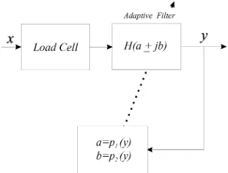
The elements of can be calculated for different values of the measurand. To emphasise that depends on , it can be written as . is unknown in the first instance when a new mea-surement begins. Therefore, the parameters of the adaptive filter cannot be set to appropriate values in order that the filter be-haves as an inverse system. Hence, an adaptive rule is required to modify the parameters of the adaptive filter according to the value of measurand. This rule is a crucial element, but there is not a straightforward solution for it. Usually, in classic adaptive techniques, an adaptive algorithm, such as a least mean squares (LMS) method, updates to minimize a cost function. How-ever, (2) shows that, for a load cell, the suitable filter has a pair of conjugate zeros , which and can be considered as the parameters of adaptive filter and the relationship between them and load can be modeled as in (3) and (4). The real-time measurement operation is shown in Fig. 2. In this block diagram, has been substituted with , the output of the whole system, which is proportional to . Initially, the zeros of the filter are set to arbitrary values. Then, the output is calculated. This new value of is used to calculate the zeros of the filter once again. Repeating these steps results in a rapid approach to obtain the steady state value of .
[image:2.594.347.508.65.187.2]So far, the zeros of the second-order compensation filter have been examined. In order that the analog filter can be realized, it
Fig. 2. Block diagram of adaptive load cell response correction.
Fig. 3. State-variable low-pass filter.
is necessary to add at least two poles to the filter. The values of these poles can be determined practically. For simulation pur-poses, these poles are selected by trial and error so that the output of the filter quickly reaches its steady-state value with minimum oscillation. The transfer function of the compensa-tion filter is
(6)
The transfer functions of the load cell (2) and its compen-sation filter (6) are biquadratic functions. There now exists a wealth of theoretical and experimental information on the de-sign of fixed or nonadaptive analog biquads [8]. The problem is how to make a biquad adaptive, and it is necessary to have only one filter component to track changes in without any influ-ence on the other parameters such as damping factor and the spring coefficient .
III. PROPOSEDLOADCELLMODEL
Amongst the various biquad structures, the state-variable lowpass filter [8], shown in Fig. 3, can be used to model the behavior of the load cell. The state-variable filter transfer function is
(7)
where
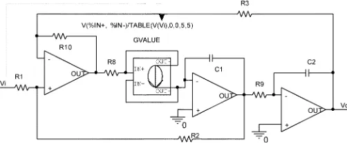
[image:2.594.303.554.224.339.2]Fig. 4. Load cell model.
Comparing this transfer function with the load cell transfer func-tion, (2), shows that can model ( ). has to be split into a fixed resistor equal to and an additional resistor pro-portional to . Since is the mass being weighed, and in the model it is equivalent to stimulating voltage ( ), the resistor has to be a voltage-controlled device whose resistance should be directly proportional to . The practical implementation of such a resistor will be discussed in Section VI. For simulation purposes, the analog behavioral modeling facility in PSPICE can be used. This is achieved by using the component (a voltage-controlled current source) and ”TABLE,” which allows the user to enter different resistors for different voltages. Using this voltage-controlled resistor in the lowpass filter (Fig. 3) pro-duces an analog biquadratic filter which can model the behavior of the load cell. The complete model is depicted in Fig. 4. From experimental data for a particular load cell [4], the damping factor , spring constant , and the effective mass of the load cell are 3.5, 2700 Pa, and 0.5 kg, respectively. These num-bers are used to determine the values for resistors and capacitors in Fig. 4.
For step excitation, the input voltage of the model is a step function whose amplitude is proportional to . The simulation results for two different values of are shown in Figs. 6 and 7, which indicate that changing the input ( similar to the prac-tical case ) varies all inertial parameters of the output waveform such as the steady state value, resonant frequency, and damping factor.
IV. PROPOSEDADAPTIVECOMPENSATIONFILTERMODEL
Since the transfer function of the compensation filter (6) is a biquadratic function, different scaled outputs in the state vari-able filter, shown in Fig. 3, need to be added to form a complete biquad. To make this biquad adaptive, as described in the block diagram of Fig. 2, the filter’s zeros have to be changed by the output of the biquad. Similar to the sensor model approach, it is possible to use a voltage-controlled resistor in the compensation filter. The filter output voltage is used to control this resistance. The complete adaptive biquad is shown in Fig. 5. The transfer function of this filter is
(9)
where
(10)
Fig. 5. Adaptive compensation filter model.
and was previously defined in (8). Similar to the sensor model, consists of a fixed resistor and a voltage-controlled resistor whose resistance is controlled by the filter’s output voltage. In other words, models ( ) in (6).
The adaptation sequence will now be described in detail. Be-fore stimulating the load cell, the filter output voltage is zero, and the initial transfer function of the filter will be
(11)
Where is the gain factor of the filter, and are the real and imaginary parts of filter’s zeros respectively, and are real and imaginary parts of filter’s poles, respectively, and the subscript ( ) denotes the initial values. The zeros of the filter need to cancel the poles of the sensor, i.e., and are the same as (3) and (4). Since (the output of the filter) is unknown at first, the values of and , which depend on , cannot be fixed. The initial values for and are
When the input is applied to the filter with initial transfer func-tion of , it produces an output, say . Since the zeros of the filter change with the output voltage, the new values for and will be and , and then the transfer function of the filter changes to
(12)
With this new transfer function, the filter produces a new output that changes the filter’s zeros again and this procedure continues until and converge to their final values.
It should be noted that the poles of this compensation filter (9) vary as varies, which is not the case with the filter model (6). However, detailed analysis has shown [9] that the filter remains stable for all values of .
V. SIMULATIONRESULTS
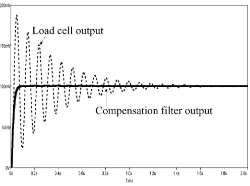
[image:3.594.38.289.65.174.2]Fig. 6. Simulation result of adaptive compensation form = 0:1kg.
Fig. 7. Simulation result of adaptive compensation form = 1kg.
in Fig. 5) can be used to correct the response of a second-order sensor system.
VI. PRACTICALIMPLEMENTATION
In the sensor and compensation models (Figs. 4 and 5), there is a floating linear voltage-controlled resistor (VCR) which must be directly proportional to the controlling voltage over a wide range because this resistor is equivalent to ( ), as described in Sections III and IV. In PSPICE simulation, this VCR was modeled using a voltage-controlled current source whose voltage values and resistors were set by a theoretical table format, hence, there was no restrictions. In practice, however, such component does not exist. The challenging part of the practical implementation of the sensor and compensation filter models is the realization of such a VCR. The properties of this VCR can be summarized as follows.
• The resistor should be floating (none of its terminals is connected to ground or power supply).
• The resistor should be linear (linear relationship between voltage and current).
between gate and source. There are, however, two major prob-lems: 1) voltage across the channel should be small, i.e., for large , the channel is a nonlinear resistor and 2) channel resistance is inversely proportional to gate voltage. There have been some papers that address linearizing the current and voltage relationship (the first problem) [10], [14], [13], and [11]. However, an extensive literature search has shown that there is very little or no work in the area of producing a resistor that varies with input voltage in a linear manner. In this section, these two problems are addressed and a novel linearization technique is proposed to solve the second one.
The relationship between drain current, , and drain–source voltage, , of a JFET in the triode or ohmic region [
] is
(13)
which shows a nonlinear relationship between and (a nonlinear resistance). For small values of , the square term in (13) can be ignored and in this case the drain–source resis-tance can be considered as a linear resisresis-tance, which in practice limits the voltage across the resistance to several hundred milli-volts. It is possible to have a linear resistance over a wider range [10], [14], [13], and [11]. However, since in the analog adaptive filter model, the voltage across VCR is very small; in (13) can be ignored without any significant impact. In this case, for less than , the channel resistance becomes
(14)
where is the minimum resistance for
. Equation (14) shows that is inversely propor-tional to controlling voltage . Equation (14) can be rewritten as
Fig. 8. Nonlinear amplifier which provides the gate voltage fromV .
Fig. 9. Implementation of the proposed piecewise linear approximation technique.
obtained as follows. The VCR needs to change linearly with , i.e.,
(16)
where is a proportional constant. The relationship between of the JFET with its is given in (14), and it is required that this resistance changes linearly with . In other words, (14) and (16) should be equal
(17)
The value of is not important, and it is assumed . By manipulating (17), the input-output relationship of the nonlinear amplifier is
(18)
One possible implementation of (18) is shown in Fig. 9, which realize piecewise linear approximation of this equation. This cir-cuit has different gains for different intervals (
)
for (19)
To calculate the gains, (18) can be approximated by straight lines, as shown in Fig. 10, for . The breaking points of
this curve are (for ).
[image:5.594.62.266.146.350.2]Corresponding inputs of the nonlinear amplifier can be cal-culated from (18). This approximation is equivalent to piece
Fig. 10. Piecewise linear approximation of (18).
Fig. 11. Linearization ofR using the proposed piecewise linear technique.
of straight lines and, hence, needs an amplifier with different gains. Slopes of the piecewise lines are equal to the gains of amplifie
m for
(20)
where .
Having used this piecewise linear amplifier to provide the gate voltage, Fig. 11 shows of the JFET with changing . To indicate the effectiveness of the proposed technique, the ideal linear case and nonlinear case are also depicted. This figure shows that can be controlled linearly over a wide range (more than three times ). In other words, the adaptive compensation filter can be used for the values of as large as
.
B. Experimental Results
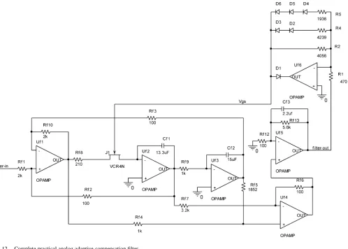
[image:5.594.306.551.290.471.2]Fig. 12. Complete practical analog adaptive compensation filter.
Fig. 13. Input and output of the adaptive filter withm = 0:1kg.
been implemented with a cascade of single diodes. For prac-tical testing, a square wave excitation voltage was applied to the sensor circuit, and according to the amplitude of the excitation voltage, the sensor VCR ( ) was changed manually. Figs. 13 and 14 show two sample inputs and outputs of the adaptive filter. The input amplitudes are 100 and 330 mV, which are equivalent to 0.1 and 0.33 kg. Clearly, the practical results show that the analog adaptive biquad filter (Fig. 12) can be used to correct the response of the load cell. It should be noted that there is good
Fig. 14. Input and output of the adaptive filter withm = 0:33kg.
[image:6.594.43.312.440.615.2]Fig. 15. Input and output of the nonadaptive filter withm = 0:33kg.
practice, careful selection is needed to achieve good correction performance.
VII. CONCLUDINGREMARKS
This paper has shown that it is possible to perform effec-tive response compensation of dynamic sensors using analog adaptive filter techniques. This has been demonstrated with a reference to a load cell sensor. It has been shown that the state-variable biquadratic filter provides an accurate and flexible sensor and adaptive compensation filter models. Simulation and experimental results, showing the viability of the proposed technique, were presented. The practical prototype consisted of a novel piecewise linearization technique for floating voltage-controlled resistor. We are currently developing circuit techniques that allow the integrated fabrication of the analog adaptive filter.
REFERENCES
[1] J. E. Brignell and N. M. White,Intelligent Sensor Systems. London, U.K.: Inst. of Physics, 1994.
[2] J. E. Brignell, “Software techniques for sensor compensation,”Sens. Ac-tuators, vol. 25–27, pp. 29–35, 1991.
[3] W. J. Shi, N. M. White, and J. E. Brignell, “Adaptive filters in load cell response correction,”Sens. Actuators, vol. A 37–38, pp. 280–285, 1993. [4] S. M. T. Alhoseyni, A. Yasin, and N. M. White, “The application of arti-ficial neural network to intelligent weighing systems,”Proc. IEE—Sci., Meas. Technol., vol. 146, pp. 265–269, Nov. 1999.
[5] M. Halimic and W. Balachandran, “Kalman filter for dynamic weighing system,” inProc. IEEE Int. Symp. Industrial Electronics, Jul. 1995, pp. 787–791.
[6] W.-Q. Shu, “Dynamic weighing under nonzero initial condition,”IEEE Trans. Instrum. Meas., vol. 42, no. 4, pp. 806–811, Aug. 1993. [7] A. Carusone and D. A. Johns, “Analogue adaptive filters: Past and
present,”Proc. IEE—Circuits, Devices, Syst., vol. 47, no. 1, pp. 82–90, Feb. 2000.
[8] W.-K. Chen,Passive and Active Filters. New York: Wiley, 1986. [9] M. Jafaripanah, B. M. Al-Hashimi, and N. M. White, “Load cell
re-sponse correction using analog adaptive techniques,” inProc. IEEE Int. Symp. Circuits Systems (ISCAS), Bangkok, Thailand, May 2003, pp. IV752–IV755.
[10] K. Nay and A. Budak, “A voltage-controlled resistance with wide dy-namic range and low distortion,”IEEE Trans. Circuits Syst, vol. CAS-30, no. 10, pp. 770–772, Oct. 1983.
[11] “FETS as voltage-controlled resistor,” Siliconix, Santa Clara, CA, AN105, 1997.
[12] R. Senani and D. R. Bhaskar, “Versatile voltage-controlled impedance configuration,”Proc. IEE —Circuits, Devices, Syst., vol. 141, no. 5, pp. 414–416, Oct. 1994.
[13] , “A simple configuration for realizing voltage-controlled imped-ances,”IEEE Trans. Circuits Syst., vol. 39, no. 1, pp. 52–59, Jan. 1992. [14] N. Tadic, “A floating, negative-resistance voltage-controlled resistor,” in
Proc. IEEE Instrumentation Measurement Technology Conf., Budapest, Hungry, May 2001, pp. 437–442.
Mehdi Jafaripanah received the B.S. degree in communication engineering from Iran University of Science and Technology, Tehran, Iran, in 1990 and the M.S. degree in electronic engineering from the Amirkabir University of Technology, Tehran, Iran, in 1994. He is currently pursuing the Ph.D. degree in the School of Electronics and Computer Science, University of Southampton, U.K.
He was an Instructor at Amirkabir University, Tafresh campus, Iran, for seven years. His main research interests are analog signal processing and switched-current circuit design for system-on-chip applications.
Bashir M. Al-Hashimi (M’99–SM’01) received the B.Sc. degree with first-class classification in electrical and electronics engineering from the Uni-versity of Bath, Bath, U.K., in 1984, and the Ph.D. degree from York University, York, U.K., in 1989.
Following his Ph.D. degree, he worked in industry for six years designing high performance chips for analog and digital signal processing applications. In 1999, he joined the School of Electronics and Com-puter Science, Southampton University, U.K., where he is currently a Professor of Computer Engineering. His research interests include low-power SoC design and test, and VLSI CAD. He has authored and coauthored over 125 technical papers and three books.
Dr Al-Hashimi is the Editor-in-Chief of theIEE Proceedings: Computers and Digital Techniquesand a Fellow of the Institution of Electrical Engineers (IEE).
Neil M. White(M’01–SM’02) received the Ph.D. degree in 1988 for a thesis on the application of thick-film piezoresistors for load cells from the De-partment of Electronics, University of Southampton, U.K.
He is a Professor of Intelligent Sensor Systems in the School of Electronics and Computer Science and Director of the Institute of Transducer Technology at the University of Southampton. He was appointed as a Lecturer in 1990, a Senior Lecturer in 1999, a Reader in 2000, and currently holds a Personal Chair. He has published extensively in the area of thick-film sensors and intelligent in-strumentation and is author or coauthor of over 100 scientific publications.