hierarchies
.
White Rose Research Online URL for this paper:
http://eprints.whiterose.ac.uk/132827/
Version: Accepted Version
Article:
Fu, W and Nijhoff, FW (2018) Linear integral equations, infinite matrices, and soliton
hierarchies. Journal of Mathematical Physics, 59 (7). 071101. ISSN 0022-2488
https://doi.org/10.1063/1.5046684
This is an author produced version of a paper published in Journal of Mathematical
Physics. Uploaded in accordance with the publisher's self-archiving policy.
[email protected] https://eprints.whiterose.ac.uk/
Reuse
Items deposited in White Rose Research Online are protected by copyright, with all rights reserved unless indicated otherwise. They may be downloaded and/or printed for private study, or other acts as permitted by national copyright laws. The publisher or other rights holders may allow further reproduction and re-use of the full text version. This is indicated by the licence information on the White Rose Research Online record for the item.
Takedown
If you consider content in White Rose Research Online to be in breach of UK law, please notify us by
AND SOLITON HIERARCHIES
WEI FU AND FRANK W NIJHOFF
Abstract. A systematic framework is presented for the construction of hierarchies of soliton equations. This is realised by considering scalar linear integral equations and their representations in terms of infinite matrices, which give rise to all (2+1)- and (1+1)-dimensional soliton hierarchies associated with scalar differential spectral problems. The integrability characteristics for the obtained soliton hierarchies, including Miura-type transforms,
τ-functions, Lax pairs as well as soliton solutions, are also derived within this framework. Keywords: linear integral equation, infinite matrix, soliton hierarchy,τ-function, Lax pair, soliton
1. Introduction
Integrable nonlinear partial differential equations (PDEs) arise in a variety of areas in modern mathematics and physics. Over the past few decades, there have been many methods developed for the construction and solutions for such equations, including inverse scattering method, Riemann–Hilbert approach, finite-gap inte-gration, Hirota’s bilinear method and methods based on representation theory, cf. the monographs [1,15,20,33]. Among those models, the Kadomtsev–Petviashvili (KP) hierarchy is often considered to be the most funda-mental one and the most popular construction of this hierarchy is Sato’s approach based on pseudo-differential operators [39]. This is related to the observation that the KP hierarchy is closely related to infinite-dimensional Grassmannians [38]. This idea was further developed by Date, Jimbo, Kashiwara and Miwa who classified soliton equations by using transformation groups associated with infinite-dimensional Lie algebras based on the so-called fundamental bilinear identity leading to the hierarchy of equations in Hirota’s form in terms of the
τ-function (cf. e.g. [19, 27] and references therein for the original research papers by the Kyoto school). The pseudo-differential operator approach may have some disadvantages. One disadvantage is that it singles out a preferred independent variable from all the flow variables in the hierarchy whereas the latter can be considered all to be on the same footing. The other disadvantage is that it can only be discretised to obtain semi-discrete equations but no fully-discrete equations have been obtained yet from this approach. In contrast, in this paper we will promote the direct linearisation (DL) approach for treating the KP hierarchy in which no preselected independent variable is required to set up the constitutive relations, and which also allows in a natural way to a full discretisation.
The DL was first proposed by Fokas and Ablowitz in [9] for solving the Korteweg–de Vries (KdV) and Painlev´e II equation, and later extended to the KP equation in [10] and some other nonlinear equations in [2, 37]). The idea behind the DL approach, to use a general linear singular integral equations in the spectral variable as the starting point, was developed further in a series of papers, cf. e.g. [28,30,32,35]. As a powerful tool to treat these linear integral equations, an infinite matrix structure was introduced, cf. [13, 28, 30], which allows to capture whole Miura-related families of equations together with their hierarchies, within one framework. Furthermore, in this framework, all the independent variables (discrete as well as continuous) are treated on the same footing. In a recent paper [13] the DL was established for the three families of the discrete KP-type equations, namely the discrete AKP, BKP and CKP equations, extending the earlier results on discrete KP equations of A-type [29]. Based on the new insights provided by the previous paper, in the current paper we revisit the continuous hierarchies for the AKP, BKP and CKP equations as well as their dimensional reductions. The resulting (1+1)-dimensional hierarchies include the following examples: the KdV, Boussinesq (BSQ), generalised Hirota– Satsuma (gHS), Hirota–Satsuma (HS), Sawada–Kotera (SK) and Kaup–Kupershmidt (KK), bidirectional SK (bSK) and bidirectional KK (bKK), and Ito hierarchies. The DL framework is presented in the language of infinite matrices and this treatment provides the following: i)different nonlinear forms in the each class together with the Miura-type transforms; ii)the multilinear form in terms of the τ-function for each class;iii)the Lax pairs of both nonlinear equations and the multilinear equation for each class;iv)the soliton solutions for both nonlinear and multilinear equations. In spite of the undeniable virtues of other approaches, we believe that the DL framework provides the most comprehensive treatment of all these results.
The paper is organised as follows: In Section 2 we set up the ingredients of the infinite matrix structure and explain the DL scheme in this language. Section 3 is contributed to the three important (2+1)-dimensional soliton hierarchies, namely, the AKP, BKP and CKP hierarchies. The dimensional reductions of the higher-dimensional models are discussed in Section 4 which includes a number of (1+1)-higher-dimensional integrable models. Finally in Section 5, soliton solutions for all the soliton hierarchies will be given as particular cases as the general DL framework.
2. Infinite matrices and linear integral equations
2.1. Infinite matrices and vectors. The details of infinite matrices can be found in [13]. In this subsection we only give a brief introduction to the notion which include all the properties and operations we need in the paper.
We first of all introduce three fundamental objectsΛ,tΛandOand they obey the relation O·tΛi·Λj·O=δ
−i,−jO, ∀i, j∈Z,
(2.1)
where tΛi and Λj mean theith andjth compositions oftΛand Λ respectively. In particulartΛ0 and Λ0 are
defined as the identities and the relation in this case reads O2 =O, namely, the objectO is a projector. In
general, Λ, tΛ and Odo not commute with each other but they commute with the elements from a suitably
chosen field of functions F which will be determined later. We consider infinite matrices of the form: U is defined as
U= X
i,j∈Z
Ui,jΛ−i·O·tΛ−j,
(2.2)
where Ui,j are elements in the field F. Here Ui,j can be understood as the entries in the infinite matrix,
while Λ−i·O·tΛ−j with i, j ∈
Z can be thought of as a basis in this infinite matrix space. In fact, it can be verified that the infinite matrices defined in this way constitute a linear space where the addition and the scalar multiplication are the same as those in the finite case. The multiplication of two infinite matrices is also well defined if one follows the rule (2.1) that the objects must obey. The transposition of U is defined as tU= P
i,jUi,jΛ
−j·O·tΛ−i. IfU =tU, comparing the coefficients (i.e. the matrix entries) of them, we
immediately have Ui,j = Uj,i. Likewise, we have Ui,j = −Uj,i if U =−tU. These results coincide with the
properties in finite matrices. Furthermore, one can introduce the action (·)0,0 on an arbitrary infinite matrix
defined by taking the coefficient ofΛ0·O·tΛ0in the definition of an infinite matrix. TakingUdefined in (2.2)
as an example, we have that
(Λi0·U·tΛj0)
0,0=Ui0,j0, ∀i0, j0∈Z.
(2.3)
As the notion of infinite matrices have been defined, we now define infinite vectors. Suppose oand toare
two vectors obeying the relations
to·tΛi·Λj·o=δ
−i,−j, o·to=O, i, j∈Z.
(2.4)
An infinite vectoruand its adjoint vectortuare defined as
u=X
i∈Z
u(i)Λ−i·o, tu=X i∈Z
u(i)to·tΛ−i,
(2.5)
where u(i) are elements in the same field F. Following the rules in (2.4), it can easily be verified that the
addition, the scalar multiplication of infinite vectors as well as the multiplication of an infinite vector and an adjoint vector are all well-defined, i.e. the addition of two infinite vectors is still an infinite vector, an infinite vector multiplied by a scalar quantity is still an infinite vector, and the multiplication of an infinite vector and an adjoint vector is an infinite matrix while the multiplication of an adjoint vector and an infinite vector is a scalar quantity. It is similar to the case in infinite matrices that we can also define the action (·)0as taking the
coefficient ofΛ0·ofor an arbitrary infinite vectoruand that ofto·tΛ0 for an arbitrary adjoint infinite vector turespectively. For instance, one can deduce that
(Λi0
·u)0=u(i0), (tu·tΛj0)0=u(j0), ∀i0, j0∈Z.
The multiplication of an infinite matrix and an infinite vector is also well-defined if one follows from (2.1) and (2.4). It obeys exactly the same rules as those in the theory of finite matrices and vectors. In other words,U·u
is an infinite vector andtu·Uis an adjoint infinite vector.
usual way and in the case of having the projectorO, the issue of convergence of summations in the definitions no longer appears. We can easily verify that the trace obeys the property Tr(U·O) = Tr(O·U) = (U)0,0.
Besides, we also have Tr(U+V) = TrU+ TrVas well as Tr(U·V) = Tr(V·U). As for the determinant of infinite matrices, we have
det(1 +U·O·V) = det(1 +U·o·to·V) = 1 +to·V·U·o= 1 + (V·U) 0,0,
whereU·oandto·Vare thought of as an infinite vector and an adjoint infinite vector respectively and (2.1)
and (2.4) are used. This identity is an infinite version of the important formula det(1 +a·bT) = 1 +bT·a
for finite column vectors a,b, namely, the Weinstein–Aronszajn formula in rank 1 case, which evaluates the determinant of an infinite matrix in terms of a scalar quantity.
2.2. Infinite matrix representation of linear integral equations. The starting point in the framework is a linear integral equation associated with (2+1)-dimensional integrable systems:
uk+
Z Z
D
dζ(l, l′
)ρkΩk,l′σl′ul=ρkck,
(2.6)
where dζ(l, l′) is a certain measure for the double integral on a domainDin the space of the spectral variablesl
andl′. The wave functionuk=P i∈Zu
(i) k Λ
−i·ois an infinite vector whereu(i) k =u
(i)
k (x;k) withx={xj|j∈Z +}
are C∞-functions with respect to the independent variables in x and k is the spectral parameter. ck is also
an infinite vector which is defined as ck = P i∈Zk
iΛ−i·o. While Ω
k,l′ is the Cauchy kernel for the integral
equation andρk,σl′ are the plane wave factors which will be given later when we deal with concrete equations.
One remark here is that the measure dζ(l, l′) depends onl andl′ and we must have a double integral involved.
Once the measure collapses the integral equation turns out to be a local Riemann–Hilbert problem leading to (1+1)-dimensional integrable systems and this will be done in Section 4 as dimensional reductions of higher-dimensional equations. Another remark is that actually we only need three variables to represent a (2+1)-dimensional integrable equation, but we still introduce an infinite number of variables in order to describe the whole hierarchy of a soliton equation. For instance, one can fixx1, x2as the space variables and the flexiblexj
forj∈Z+ is the time variable which denotes thejth flows in the hierarchy. The third remark is that although
uk is an infinite vector, nevertheless, the equation (2.6) is a set of many integral equations in terms of the wave functionsu(i)k . Therefore it should still be understood as a set of scalar integral equations.
Now we introduce some key quantities in the representation of the linear integral equation in terms of infinite matrices. We define the infinite matrices
C=
Z Z
D
dζ(l, l′
)ρlcltcl
′σl′, U= Z Z
D
dζ(l, l′
)ultcl ′σl′.
(2.7)
In fact, C can be understood as the infinite matrix analogue of the plane wave factor ρl and σl′ and U can
be considered as the infinite matrix version for the wave function uk. Next we define an operator Ω by Ωk,l′ = tcl′ ·Ω·ck and it is clear to see that Ω is the analogue of the Cauchy kernel in our infinite matrix
language. Consider the new quantitiesC,U andΩ, one can now represent the integral equation (2.6) as
uk = (1−U·Ω)·ρkck
(2.8)
and its nonlinear version, namely, the relation for the infinite matrixU, can be written in the form of
U= (1−U·Ω)·C.
(2.9)
Equations (2.8) and (2.9) are the fundamental relations in the DL scheme. Once Ω and C are given, one can then consider the dynamical evolutions for both quantities. By choosing entries/components inU anduk
suitably, closed-form nonlinear equations and the associated linear problems will arise. The Ω andC are also the ingredients for the τ-function which can represent the multilinear structure for the nonlinear equations. Then theUdefined as a double integral in (2.7) provides the most general solution for the obtained closed-form equations. Solutions having a particular behaviour (e.g. soliton solutions) can be constructed by taking a suitable form of the measure dζ(l, l′) and the domain D. In the paper we only consider soliton solutions of
integrable equations as they can be regarded as one of the most important characteristics of integrability. 3. (2+1)-dimensional soliton hierarchies
3.1. The AKP hierarchy. The AKP hierarchy, normally known as the KP hierarchy, is associated with the infinite-dimensional Lie algebra A∞, namely gl(∞). In this class, we consider a particular infinite matrix C
given by
C=
Z Z
D
dζ(l, l′
)ρlcltcl
′σl′, ρk= exp
∞
X
j=1
kjx j
, σk′ = exp
− ∞
X
j=1
(−k′
)jx j
,
(3.1)
where ρk and σk′ are the plane wave factors. Differentiating C with respect to xj and notice the form of ρk
andσk′, one can obtain the dynamical evolution ofC:
∂jC=Λj·C−C·(−tΛ)j, j∈
Z+,
(3.2)
where∂j=. ∂xj. The operatorΩ, namely, the infinite matrix version of the Cauchy kernel in this case is defined
by the relation
Ω·Λ+tΛ·Ω=O.
(3.3)
In fact, the Cauchy kernel can be recovered fromΩand it is now given by Ωk,l′ =k+l1′. One can now consider
the dynamical evolution ofUdefined as (2.9). In fact, making use of Equations (3.2) and (3.3), we end up with the relation forU as follow:
∂jU=Λj·U−U·(−tΛ)j−U·Oj·U, j∈
Z+,
(3.4)
where Oj =. Pj−1 i=0(−
tΛ)i·O·Λj−1−i. Equations (3.4) can be considered as the AKP hierarchy expressed by
the infinite matrixU.
Following from the definition ofOj, one can easily prove the recurrence relation
Oi+j=Oi·Λj+ (−tΛ)i·Oj.
(3.5)
Making use of the recurrence relation ofOj (3.5), one can find the recurrence relation for the dynamical relation ofU(3.4) via some straightforward computation and they are given by:
(∂i+j+∂i∂j)U= (Λi−U·Oi)·(∂jU) + (Λj−U·Oj)·(∂iU),
(∂i+j−∂i∂j)U= (∂jU)·((−tΛ)i+Oi·U) + (∂iU)·((−tΛ)j+Oj·U).
The importance of the above relations is that in the first one only Λis involved and in the second one onlytΛ
is involved. This observation provides us with a possibility to reduce the degree ofΛandtΛ in the dynamical
relation ofU, i.e. (3.4). In fact, takingi=j= 1, one can have
Λ·U=1 2∂
−1
1 (∂2U+∂12U+ 2U·O·(∂1U)),
(3.6a)
U·(−tΛ) = 1 2∂
−1
1 (∂2U−∂12U−2(∂1U)·O·U).
(3.6b)
With the help of Equation (3.6), one can eliminateΛandtΛin (3.4) and obtain a differential relation for only Uand O. Consider the entryU0,0= (U)0,0=. uin the infinite matrixU, the KP (i.e. AKP) hierarchy can be
derived. The first nontrivial equation (whenj= 3), namely, the KP equation, is given by
ux3x1 = 1
4ux1x1x1+
3 2u
2 x1
x1
+3 4ux2x2.
(3.7)
We note that a slightly different derivation of the KP equation (3.7) from the DL framework can be found in [43]. Other nonlinear forms in the AKP class can also be derived if one defines v = [ln(1−U0,−1)]x1,
w=−U1,−1/(1−U0,−1) andz=U−1,−1−x1. In fact, (3.4) leads to some Miura-type transforms between these
variables:
2ux1 =−vx1−v 2+∂−1
x1vx2, v=
1 2
zx1x1+zx2
zx1
.
(3.8)
We omit the derivation of these transforms and one can verify these identities by substituting the derivatives with the entries in the infinite matrixUby using (3.4). By these transforms, one can from (3.7) derive
vx3x1 = 1
4vx1x1x1−
3 2v
2v x1
x1
+3 2vx1x1∂
−1 x1 vx2+
3
2vx1vx2+
3 4vx2x2,
(3.9)
zx3
zx1
x1
=1
4{z, x1}x1+
3 4
zx2
zx1 zx2
zx1
x1
+3 4
zx2
zx1
x2
, {z, x1}=. zx 1x1x1
zx1
−3
2
z2 x1x1
z2 x1
.
The two equations are referred to as the modified KP (mKP) equation and the Schwarzian KP (SKP) equation respectively. {z, x1}defined above is the Schwarzian derivative ofzwith respect tox1and it is M¨obius invariant,
namely it is invariant under a fractionally linear transform and therefore it is clear to see that the SKP equation has a M¨obius symmetry (cf. [44]). In addition, one can also find wx1 =
1
2(vx1 −v
2+∂−1
x1vx2), which implies
that the variablewalso obeys the KP equation (3.7). One remark here is that the AKP class can be obtained from differentΩ. For instance, one can replaceO in (3.3) by 12(O·Λ−tΛ·O), thenU
0,0 will also give us a
slightly different form (a weak form) of the mKP equation.
From the above result we have seen that the AKP hierarchy has a lot of nonlinear forms. Therefore we need a quantity that can describe the evolution of the AKP hierarchy in a unified way. The τ-function defined by
τ = det(1 +Ω·C) can actually be a very good candidate as it contains the information ofΩ andC that is given at the beginning of our scheme. This reminds us of considering the dynamical evolution of theτ-function. In fact some simple calculation using the rank 1 Weinstein–Aronszajn formula shows that
∂jlnτ=∂jln(det(1 +Ω·C)) = Tr(Oj·U),
(3.11)
where in the derivation the identity ln(detW) = Tr(lnW) for an arbitrary matrixWis used. When j= 1, it gives us the multilinear transform u= (lnτ)x1 and as a result the equation (3.7) turns out to be the bilinear
equation
(D14−4D1D3+ 3D22)τ·τ = 0,
(3.12)
in which the operatorDj is the standard bilinear operator in terms of the continuous independent variablexj
defined by
Dnjf(x)·g(x
′
) = (∂xj−∂x′j)
n
f(x)g(x′
)|x′=x, x={xj|j∈Z+}, x′ ={x′j|j∈Z+}.
The higher-order equations for theτ-function can be obtained from the nonlinear AKP hierarchy inuvia the same transform. But we note that the obtained τ-equations may no longer be bilinear, instead they will be multilinear. It is this set of multilinear equations that governs the algebraic structure behind the AKP class.
In the DL framework, the fundamental object is the infinite matrixUwhich generates the whole KP hierarchy with the help of (3.4) and (3.6); more precisely, eliminating Λ and tΛ in these relations and considering the
(0,0)-entry gives us the whole KP hierarchy expressed by the nonlinear variable u. The bilinear transform
u = (lnτ)x1 then brings us a hierarchy of multilinear equations expressed by the same τ-function. These
multilinear equations are deep down equivalent to the bilinear KP equations in the Sato scheme, see e.g. [19] and [34]. The difference is that in the bilinear framework more and more independent variables must be involved in higher-order bilinear equations, but in our approach each multilinear equation only depends on three dynamical variables, namelyx1,x2 andxj.
Now we consider the linear problem of the AKP hierarchy. The differentiation of (2.8) together with Equations (3.4) and (3.3) bring us the dynamical evolution foruk in the AKP class given by
∂juk =Λj·uk−U·Oj·uk.
(3.13)
Like how we deal with the nonlinear variableU, a similar derivation provides us with the following important relations foruk:
(∂i+j−∂i∂j)uk= (∂jU)·Oi·uk+ (∂iU)·Oj·uk, j∈Z+.
By takingi=j= 1 and settingφ=u(0)k in the above relation, the linear problem can be obtained and it is as the following:
φx2 = (∂ 2
1+ 2ux1)φ.
(3.14a)
The linear equation (3.14a) inφgoverns the linear structure of the whole AKP hierarchy, namely, it is the spacial part of the Lax pairs for all the members in the AKP hierarchy. The temporal evolutions of the hierarchy can be derived by considering the corresponding flows separately. In practice, one can have from (3.13)
Λ·uk=∂1uk+U·O·uk
by takingj = 1. This relation together with (3.6) can help to reduce the order ofΛ andtΛ in∂
juk following
from (3.13) and therefore the temporal evolutions can be derived. For instance, if we consider thex3-flow in
(3.13), we have the temporal evolution
φx3= h
∂13+ 3ux1∂1+
3
2(ux1x1+ux2) i
φ.
The compatibility condition of the spacial part (3.14a) and the temporal evolution (3.14b), namely, φx2x3 =
φx3x2, gives us the KP equation (3.7). The Lax pairs for the other nonlinear and multilinear forms can be
calculated by replacinguin (3.14) by the other variables via the Miura-type transforms (3.8) and the multilinear transform. The temporal evolution of the higher-order equations in the hierarchy can be derived in a similar way.
3.2. The BKP hierarchy. The BKP hierarchy is associated with the infinite-dimensional algebraB∞ which
is a sub-algebra ofA∞, therefore the BKP hierarchy can be understood as a sub-hierarchy of AKP. In this case,
we take a particular infinite matrixC as follow:
C=
Z Z
D
dζ(l, l′
)ρlcltcl
′ρl′, ρk = exp X∞
j=0
k2j+1x2j+1
, dζ(l′
, l) =−dζ(l, l′
).
(3.15)
From the above formula one can see the difference between BKP and AKP is that in the BKP hierarchy only odd independent variables are involved and besides the measure in the integral has the antisymmetry property. One can easily find thatC satisfies the dynamical relation
∂2j+1C=Λ2j+1·C+C·tΛ2j+1, j= 0,1,2,· · ·
(3.16)
as well as the antisymmetry propertytC=−C. Now we require that the infinite matrix versionΩof the kernel
obeys the algebraic relation
Ω·Λ+tΛ·Ω=1
2(O·Λ−
tΛ·O).
(3.17)
Actually we have pointed out in the previous section that replacing the right hand side of (3.3) by12(O·Λ−tΛ·O)
also gives us the AKP hierarchy in a slightly different form. So Equation (3.17) is just another representation of (3.3). In other words, the infinite matrix relation forΩis preserved from AKP to BKP, but here we impose in addition the antisymmetry property on the measure as one can see in (3.15). We would also like to note that this actually provides us with the Cauchy kernel Ωk,l′ = 12k−l
′
k+l′ in the linear integral equation. Using
Equations (3.16) and (3.17), and differentiating the general structure of U, i.e. (2.9), one immediately obtains the dynamical evolution ofU with respect to the independent variablexj given by
∂2j+1U=Λ2j+1·U+U·tΛ2j+1−1
2U·(O2j+1·Λ−
tΛ·O2j+1)·U, j= 0,1,2,· · · .
(3.18)
In addition, it can be proven that the infinite matrixU obeys the antisymmetry propertytU=−U. This can
be derived from the antisymmetry property ofC andΩ (the antisymmetry ofΩ is obvious since the kernel is antisymmetric in kand l′). We can now refer to (3.18) together with the antisymmetry property of Uas the
BKP hierarchy in infinite matrix form because the structure of BKP (i.e. the infinite matrixCand the operator
Ω) has been contained in the two relations.
In order to get a closed-form scalar equation, we set u= U1,0 =−U0,1. Like AKP, consider x1-, x3- and
x2j+1-flows in the equation (3.18) and eliminating all the other variables apart from u, the nonlinear form of
thex2j+1-flow of the BKP hierarchy can be obtained. Among them the first nontrivial equation is thex5-flow,
which is the BKP equation, i.e.
9ux5x1−5ux3x3+ (−5ux1x1x3−15ux1ux3+ux1x1x1x1x1+ 15ux1ux1x1x1+ 15u 3
x1)x1 = 0.
(3.19)
Other nonlinear forms (e.g. the modified BKP equation, etc.) in the BKP class also exist like AKP, but multi-component forms must be involved. We omit them here because we would prefer to be focusing on scalar nonlinear forms.
Theτ-function in the BKP class is defined asτ2= det(1 +Ω·C). The reason why we defineτ2here instead
of τ is because the determinant must be in the form of a perfect square due to the antisymmetry property of Ω and C and this treatment will lead to the equations in τ written in a more elegant form. Some direct computation yields the dynamical evolution of ∂2j+1lnτ2 and the simplest one gives rise to the transform
(lnτ2)
x1 = 2(lnτ)x1 = u, which transfers the nonlinear BKP hierarchy to its multilinear form. The first
nontrivial multilinear equation in the hierarchy can be obtained from (3.19), which is given by (D61−5D13D3−5D23+ 9D1D5)τ·τ = 0,
(3.20)
Now we consider the linear problem for the BKP hierarchy. In fact, differentiating (2.8) with respect to
x2j+1, one has the dynamical evolution
∂2j+1uk=Λ2j+1·uk−1
2U·(O2j+1·Λ−
tΛ·O2j+1)·uk, j= 0,1,2,· · · ,
(3.21)
where (3.18) and (3.21) are used. One can refer to this relation as the linear problem for the BKP hierarchy in infinite matrix form. Similarly to the linear problem for AKP, we denote φ = u(0)k and after eliminating the other components u(i)k for i 6= 0 in Equation (3.21), one can get the linear problems for the whole BKP
hierarchy. For instance the spectral problem and the temporal evolution for the BKP equation (3.19) are given by
φx3= (∂ 3
1+ 3ux1∂1)φ,
(3.22a)
φx5= h
∂15+ 5ux1∂ 3
1+ 5ux1x1∂ 2 1+
10
3 ux1x1x1+ 5u 2 x1+
5 3ux3
∂1 i
φ.
(3.22b)
The linear problem for (3.20) can be obtained using the transformu= 2(lnτ)x1. We note that we made use
of the dynamical evolution and the antisymmetry property of the infinite matrix of Uin the derivation. The temporal parts for the other members in the hierarchy can be calculated in the same way by considering the corresponding flows in (3.21).
3.3. The CKP hierarchy. For the KP hierarchy of C-type (associated with the infinite-dimensional Lie algebra
C∞), we define the infinite matrixC as
C=
Z Z
D
dζ(l, l′
)ρlcltcl
′ρl′, ρk = exp
∞
X
j=0
k2j+1x2j+1
, dζ(l′
, l) = dζ(l, l′
).
(3.23)
From the definition one can see that the only difference between the BKP and CKP classes is that the measure is now symmetric in the CKP case. The symmetric measure immediately provides the propertyC=tC. Since
there are only odd flows in the plane wave factors in theC, the dynamical evolutions of the infinite matrixC
only involve the odd flows and they are given by
∂2j+1C=Λ2j+1·C+C·tΛ2j+1,
(3.24)
which is exactly the same as that in the BKP class. We now require that the Ω in the CKP class obeys the algebraic relation
Ω·Λ+tΛ·Ω=O.
(3.25)
This relation for the operator Ω is the same as (3.3), and this tells us that the Cauchy kernel in this case is Ωk,l′ =k+l1′. Making use of the symmetry property ofCandΩand following the definition ofU(2.9), we have
the symmetry propertytU =U. One can now consider the dynamical evolution ofUwith the help of (3.24)
and (3.25). By differentiatingUwith respect to the independent variablesx2j+1, we have
∂2j+1U=Λ2j+1·U+U·tΛ2j+1−U·O2j+1·U, j= 0,1,2,· · · .
(3.26)
The dynamical relation (3.26), together with the symmetry property of U, can be thought of as the CKP hierarchy in infinite matrix form.
We now look for scalar closed-form equations from the infinite matrix structure by choosing particular entries inU. In fact, one can takeu=U0,0and select x1, x3andx2j+1 as the independent variables for thex2j+1-flow
of the CKP hierarchy in (3.26). As a result the CKP hierarchy can be found and the first nontrivial equation is the CKP equation
9ux5x1−5ux3x3+
−5ux1x1x3−15ux1ux3+ux1x1x1x1x1+ 15ux1ux1x1x1+ 15u 3 x1+
45 4 u
2 x1x1
x1
= 0.
(3.27)
By selecting other entries in U, one can also obtain other nonlinear forms from the infinite matrix structure nevertheless the price one has to pay is that they may be in multi-component form and thus we omit them here. A unified structure describing the CKP class should be the form in theτ-function. In this case, it is defined by
whichUis symmetric. The first one of them gives us the transformu= (lnτ)x1 and therefore one obtains the
multilinear form of the CKP equation (3.27) given by 4τ3τx1x1x1x1x1x1+ 5τ
2τ2
x1x1x1−24τ 2τ
x1τx1x1x1x1x1−30τ τx1τx1x1τx1x1x1+ 45τ 2 x1τ
2 x1x1
+ 60τ τx1τx1x1x1x1−60τ 3
x1τx1x1x1+ 60τ 2τ
x1τx1x1x3−60τ τ 2
x1τx1x3+ 60τ 3
x1τx3−60τ τx1τx1x1τx3
+ 20τ2τx1x1x1τx3−20τ 3τ
x1x1x1x3+ 20τ 2τ2
x3−20τ 3τ
x3x3+ 36τ 3τ
x1x5−36τ 2τ
x1τx5= 0.
(3.28)
This quadrilinear form is analogous to the result for the discrete CKP equation (cf. e.g. [13]) which is in the form of Cayley’s 2×2×2 hyperdeterminant. In other words, Equation (3.28) can be understood as the continuous analogue of a hyperdeterminant. The multilinear transform also brings the higher-order equations inuin the hierarchy to the corresponding multilinear forms in theτ-function.
Similarly to how we derive (3.26), one can from (3.26) and (3.25) obtain the dynamical evolution of uk as follow:
∂2j+1uk =Λ2j+1uk−U·O2j+1·uk, j= 0,1,2,· · ·.
(3.29)
One can refer to these relations together withU=tU as the linear problems for the CKP hierarchy in infinite
matrix form. In fact, if we fixx3 andx1 and setφ=u(0)k , the spatial part of the linear problem is derived by
getting rid the other components inuk, and it is given by
φx3 =
∂13+ 3ux1∂1+
3 2ux1x1
φ.
(3.30a)
This is the spacial part for the whole CKP hierarchy. The temporal part can also be calculated from (3.29) as well. For the CKP equation (3.28), namely the time variable is fixed atx5, we have the temporal evolution
φx5 = h
∂15+ 5ux1∂ 3 1+
15 2 ux1x1∂
2 1
+35
6 ux1x1x1+ 5u 2 x1+
5 3ux3
∂1+ 5
3ux1x1x1x1+ 5ux1ux1x1+
5 6ux1x3
i
φ.
(3.30b)
The temporal evolutions for the higher-order equations in the hierarchy can be obtained similarly but the formulae of them become more and more complex.
4. (1+1)-dimensional soliton hierarchies
Dimensional reductions of higher-dimensional hierarchies can always be thought of a powerful tool to obtain (1+1)-dimensional integrable hierarchies. In general, following Sato’s scheme, such reductions are normally done by imposing certain conditions on pseudo-differential operators and consequently the Lax operators for the corresponding lower-dimensional hierarchies arise, cf. e.g. the Kyoto school [27], Konopelchenko and Strampp [23,24], Cheng and Li [5], and also Loris and Willox [25,26], etc. Among these dimensional reductions, some of them give rise to integrable systems associated with matrix or nonlocal scalar Lax structure which we think will arise from the view point of the DL starting from a matrix linear integral equation. We do not discuss these systems in the current paper and only consider the dimensional reductions leading to scalar differential spectral problems.
Dimensional reductions can also be realised within the DL framework. As we can see in the previous section, the integral equation associated with (2+1)-dimensional soliton hierarchies is a nonlocal Riemann– Hilbert problem, namely, there must be a double integral in it. When the double integral collapses, the integral equation turns out to be a local Riemann–Hilbert problem which is associated with (1+1)-dimensional soliton models. This method was recently used in [48] in order to construct an extended discrete BSQ equation and under such reductions more general solutions can be found for the obtained reduced soliton hierarchies. In this section, we generalise this method generically to the AKP, BKP and CKP hierarchies and as a result we obtain a huge class of (1+1)-dimensional soliton hierarchies.
4.1. Dimensional reductions of the KP-type hierarchies.
Reductions of the AKP hierarchy. We take the measure in a particular form as dζ(l, l′
) =
N X
j=1
dλj(l)dl′δ(l′+ωjl),
whereω is the Nth root of unity, namely,ωN = 1. The linear integral equation for the AKP hierarchy with a
double integral then turns out to be an integral equation with only a single integral as follow:
uk+
N X
j=1 Z
Γj
dλj(l)
ρkσ−ωjl
k−ωjlul=ρkck, ρk= exp X∞
j=1
kjx j
, σk′ = exp
− ∞
X
j=1
(−k′
)jx j
,
(4.2)
where Γj is a certain contour (as degeneration of the domain D) for the integral and dλj(l) is the associated
measure. This integral equation is the one for theNth member in the Gel’fand–Dikii (GD) hierarchy. In fact, such a reduction imposed on the AKP hierarchy also gives reduced forms of the infinite matrix C and the infinite matrixUrespectively:
C=
N X
j=1 Z
Γj
dλj(l)ρlcltc−ωjlσ−ωjl, U=
N X
j=1 Z
Γj
dλj(l)ultc−ωjlσ−ωjl.
(4.3)
Nevertheless, one can easily verify the representation ofUin terms of the infinite matrices (2.9) will be invariant, i.e. we still haveU= (1−U·Ω)·U, and so is that ofuk (2.8), namely, uk = (1−U·Ω)·uk. The same thing will also happen in the dimensional reductions of the BKP and CKP hierarchies.
Consider the property of theNth root of unity, we can obviously see from the structure of theC, i.e. Equation (4.3), thatC satisfies not only the dynamical relation (3.2) but also the following algebraic relation:
∂jC=Λj·C−(−tΛ)j·C= 0, j= 0 modN.
(4.4)
In other words, from the view point of the DL framework, some dynamical relations degenerate to algebraic relations. This observation immediately leads to a similar property for the nonlinear variableUwhich is given by
∂jU=Λj·U−U·(−tΛ)j−U·Oj·U= 0, j= 0 modN.
(4.5)
In fact, this algebraic relation can be proven by differentiating (2.9) with respect toxj and making use of (3.3)
(which is invariant under the reduction), (3.2) and (4.4). Equations (3.4) together with (4.5) can be considered as the hierarchy in GD of rankN in infinite matrix form. Furthermore, for the multilinear variableτ one can easily derive the constraints∂jτ = 0 forj= 0 mod N due to (4.3) and the variableuk for the linear problem
now obeys the algebraic relation
∂juk=Λj·uk−U·Oj·uk=kjuk, j= 0 modN,
(4.6)
which together with (3.13) will provide the Lax pairs for the reduced (1+1)-dimensional hierarchies.
Reductions of the BKP hierarchy. In the BKP class, we introduce the reduction of the measure in a slightly different way, which is given by
dζ(l, l′
) =
N X
j=1
dλj(l)dl′δ(l′+ωjl)− N X
j=1
dλj(l′)dlδ(l+ωjl′).
(4.7)
The reason why we take this more complex form compared to (4.1) is because in the BKP hierarchy the measure dζ(l, l′) is antisymmetric and only the dimensional reduction (4.7) can preserve the property. Like the reductions
of AKP, we have that in the BKP hierarchy the reduced integral equation is given by
uk+
N X
j=1 Z
Γj
dλj(l)
1 2ρk
k+ωjl
k−ωjlρ−ωjlul−
N X
j=1 Z
Γj
dλj(l′)
1 2ρk
k−l′
k+l′ρl′u−ωjl=ρkck.
(4.8)
And the reduced infinite matrixC becomes
C=
N X
j=1 Z
Γj
dλj(l)ρlcltc−ωjlρ−ωjl−
N X
j=1 Z
Γj
dλj(l′)ρ−ωjl′c−ωjl′tcl′ρl′,
(4.9)
where ρk = exp(P
∞
j=0k2j+1x2j+1) and obviously it still obeys tC = −C. Simultaneously, for the nonlinear
variableUwe have
U=
N X
j=1 Z
Γj
dλj(l)ultc−ωjlρ−ωjl−
N X
j=1 Z
Γj
dλj(l′)u−ωjl′tcl′ρl′,
(4.10)
which also obeys the antisymmetry propertytU =−Ufollowing from that of Ω defined in (3.17) and that of
Some straightforward computation shows that the infinite matrixCin theN-reduction of the BKP hierarchy obeys
Λj·C−(−tΛ)j·C= 0, j= 0 modN,
(4.11)
and this together with (2.9) and (3.17) give rise to the algebraic relation for the nonlinear variableUwhich is given by
Λj·U−U·(−tΛ)j−1
2U·(Oj·Λ−
tΛ·Oj)·U= 0, j= 0 modN.
(4.12)
This relation obviously implies that∂2j+1U= 0 when 2j+ 1 = 0 modN in (3.18) and consequently we have also∂2j+1τ = 0. Similarly one can also from (2.8) prove that the reduction (4.7) gives us
kjuk=Λj·uk−1
2U·(Oj·Λ−
tΛ·Oj)·uk, j= 0 modN,
(4.13)
and particularly when 2j+ 1 = 0 modN this algebraic relation implies∂2j+1uk=k2j+1uk if one follows from
(3.21). This relation together with (3.21) will later give us the Lax pairs for the (1+1)-dimensional hierarchies arising from the reductions of the BKP class.
Reductions of the CKP hierarchy. While in the CKP class, we take a particular measure in the form of dζ(l, l′
) =
N X
j=1
dλj(l)dl′δ(l′+ωjl) + N X
j=1
dλj(l′)dlδ(l+ωjl′).
(4.14)
This reduction on the measure has been symmetrised, namely, the reduced measure preserves the symmetry property, and it in turn implies that we now have the integral equation for the reduced hierarchies from the CKP class as
uk+
N X
j=1 Z
Γj
dλj(l)
ρkρ−ωjl
k−ωjlul+ N X
j=1 Z
Γj
dλj(l′)
ρkρl′
k+l′u−ωjl=ρkck,
(4.15)
where ρk is exactly the same as the one in the reductions of BKP, namely ρk = exp(P
∞
j=0k2j+1x2j+1) . The
infinite matrixC in this case is now expressed by
C=
N X
j=1 Z
Γj
dλj(l)ρlcltc−ωjlρ−ωjl+
N X
j=1 Z
Γj
dλj(l′)ρ−ωjl′c−ωjl′tcl′ρl′,
(4.16)
and it obeys the symmetry propertytC=C. Furthermore the nonlinear variableUnow turns out to be U=
N X
j=1 Z
Γj
dλj(l)ultc−ωjlρ−ωjl+
N X
j=1 Z
Γj
dλj(l′)u−ωjl′tcl′ρl′,
(4.17)
and due to the symmetry property ofC andΩin the reductions, from (2.9) one still hastU=U.
Notice thatωN = 1, one can easily prove that the infinite matrixCobeys the algebraic relation Λj·C−(−tΛ)j·C= 0, j= 0 modN,
(4.18)
which is exactly the same as the one in the reductions of BKP, i.e. (4.11), and consequently one can now follow from (2.9) and obtain the important algebraic relation for the nonlinear dynamical variableUas follow:
Λj·U−U·(−tΛ)j−U·Oj·U= 0, j = 0 modN.
(4.19)
In the particular case when 2j+ 1 = 0 modN, this above algebraic relation yields ∂2j+1U= 0. While from (4.18) we can prove∂2j+1C= 0 and consequently∂2j+1τ= 0 in the same case.
On the linear level, taking (4.19) into consideration, one can find from (2.8) that the linear variable uk
satisfies the algebraic relation
kjuk=Λj·uk−U·Oj·uk, j= 0 modN,
(4.20)
which implies∂2j+1uk =k2j+1uk when 2j+ 1 = 0 modN and this relation is the ingredient for Lax pairs of
the reduced lower-dimensional equations.
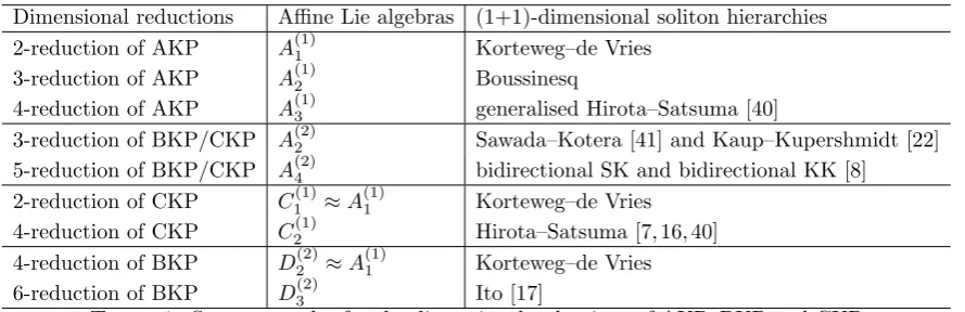
Dimensional reductions of the KP-type equations are associated with finite-dimensional Kac–Moody Lie algebras as sub-algebras of A∞, B∞ and C∞ [19]. Table 1 shows the first few examples of the dimensional
Dimensional reductions Affine Lie algebras (1+1)-dimensional soliton hierarchies 2-reduction of AKP A(1)1 Korteweg–de Vries
3-reduction of AKP A(1)2 Boussinesq
4-reduction of AKP A(1)3 generalised Hirota–Satsuma [40]
3-reduction of BKP/CKP A(2)2 Sawada–Kotera [41] and Kaup–Kupershmidt [22]
5-reduction of BKP/CKP A(2)4 bidirectional SK and bidirectional KK [8]
2-reduction of CKP C1(1)≈A(1)1 Korteweg–de Vries 4-reduction of CKP C2(1) Hirota–Satsuma [7, 16, 40] 4-reduction of BKP D(2)2 ≈A
(1)
1 Korteweg–de Vries
[image:12.595.78.523.85.229.2]6-reduction of BKP D(2)3 Ito [17]
Table 1. Some examples for the dimensional reductions of AKP, BKP and CKP
DL scheme for the hierarchies of all the equations listed in the table as examples according to the generic scheme for the dimensional reductions given in this subsection.
4.2. The Korteweg–de Vries hierarchy. The KdV hierarchy is from the 2-reduction of the AKP hierarchy. The general scheme for KdV is given by the dynamical relation and the algebraic relation
∂2j+1U=Λ2j+1·U+U·tΛ2j+1−U·O2j+1·U, j= 0,1,2,· · · ,
(4.21a)
Λ2·U−U·tΛ2−U·O2·U= 0.
(4.21b)
These relations constitute the infinite matrix version of the KdV hierarchy. In order to obtain some closed-form equations, namely some scalar equations, from the scheme, we take u=U0,0, v = [ln(1−U0,−1)]x1 and
z=U−1,−1−x1and these variables give rise to the KdV, modified KdV (mKdV) and Schwarzian KdV (SKdV)
hierarchies. The first nontrivial equation (whenj= 1 in (4.21a)) in the KdV hierarchy is the KdV equation:
ux3 =
1
4ux1x1x1+
3 2u
2 x1.
(4.22)
From (4.21a) and (4.21b) one can also find the connection betweenuandvas well as that betweenvandz, i.e. the Miura-type transforms among the nonlinear variables given by
ux1=−
1
2(vx1+v
2), v= 1
2
zx1x1
zx1
.
(4.23)
The above transforms help us to derive other nonlinear forms in the KdV class from (4.22) and we find
vx3 =
1
4vx1x1x1−
3 2v
2v x1,
(4.24)
zx3
zx1
= 1 4{z, x}
.
=1 4
zx1x1x1
zx1
−3
8
z2 x1x1
z2 x1
.
(4.25)
The equation in v is the mKdV equation and the equation inz is the SKdV equation. Actually, since the 2-reduction of AKP is equivalent to∂2U= 0 as we have pointed out in Subsection 4.1, the above results can very easily be obtained from the results in the AKP class discussed in Subsection 3.1. The higher-order equations in the mKdV and SKdV hierarchies can be calculated via the same Miura-type transforms.
The τ-function of the KdV class is the same as the one for the AKP class with an additional constraint
∂2jτ = 0. Therefore the same transformu= (lnτ)x1 substituted into (4.22) gives us the bilinear KdV equation
(D41−4D1D3)τ·τ= 0,
(4.26)
which can also be obtained from (3.12) directly by reduction.
The infinite matrix version of the linear problem of the KdV hierarchy can be obtained from the reduction of that for the AKP hierarchy and it is given by
k2uk=Λ2·uk−U·O2·uk, ∂2j+1uk=Λ2j+1·uk−U·O2j+1·uk, j= 0,1,2,· · · .
By taking φ = (uk)0, one can obtain the Lax pair for the KdV hierarchy and the one for the KdV equation
(4.22) is
LKdVφ=k2φ, LKdV=∂2
1+ 2ux1,
(4.28a)
φx3=
∂3
1+ 3ux1∂1+
3 2ux1x1
φ.
(4.28b)
Equation (4.28a) is the spectral problem for the whole KdV hierarchy. The Lax pair for the other nonlinear forms (4.24) and (4.25) and the bilinear form (4.26) can be written down if one replacesuby the other variables according the transforms given in this subsection.
The 2-reduction of the CKP hierarchy is exactly the same as the scheme from that of AKP, therefore the same results can be obtained. In fact, the additional constrainttU=Ufrom CKP (which AKP does not have)
only appears in the KdV class (N = 2) as a special case, and it is equivalent to the algebraic relation (4.21b). The 4-reduction of the BKP hierarchy is slightly different and the infinite matrix structure ofUis given by
∂2j+1U=Λ2j+1·U+U·tΛ2j+1−1
2U·(O2j+1·Λ−
tΛ·O2j+1)·U, j= 0,1,2,· · · , Λ4·U−U·tΛ4−1
2U·(O4·Λ−
tΛ·O4)·U= 0, tU=−U.
Choosing the entryu=U1,0 in the infinite matrix one can derive the KdV hierarchy and the first nontrivial
equation is ux3+ 1
2ux1x1x1 + 3 2u
2
x1 = 0 which is the same as (4.22) up to some scaling on the independent
variables and the dependent variable. The bilinear transform u = 2(lnτ)x1 according to BKP gives us the
bilinear form (D4
1+ 2D1D3)τ·τ = 0 obviously. The infinite matrix structure for the linear variableuk in this
case obeys
k4uk =Λ4·uk−1
2U·(O4·Λ−
tΛ·O4)·uk,
∂2j+1uk=Λ2j+1·U+U·tΛ2j+1−1
2U·(O2j+1·Λ−
tΛ·O2j+1)·U,
wherej= 0,1,2,· · ·, and it leads to a 4th-order Lax pair for KdV if we take φ=u(0)k :
LKdVφ=k4φ, φx3 = (∂ 3
1+ 3ux1∂1)φ,
whereLKdV=∂4
1+ 4ux1∂ 2
1+ 2ux1x1∂1.
4.3. The Boussinesq hierarchy. In this section we consider the 3-reduction of AKP. From the general struc-ture in Subsection 4.1, whenN= 3 we have the dynamical relation forUtogether with the associated algebraic relation as follows:
∂jU=Λj·U−U·(−tΛ)j−U·Oj·U, j6= 0 mod 3, j∈
Z+,
(4.29a)
Λ3·U+U·tΛ3−U·O3·U= 0.
(4.29b)
The relations constitute the infinite matrix representation of the BSQ hierarchy. In fact, these relations are equivalent to the dynamical relations for the AKP hierarchy (3.4) subject to a constraint ∂jU = 0 for j = 0 mod 3. If one introduces the nonlinear variables u =U0,0, v = [ln(1−U0,−1)]x1 and z =U−1,−1−x1, from
the (4.29a) and (4.29b) one can obtain the BSQ, modified (mBSQ) and Schwarzian BSQ (SBSQ) hierarchies respectively. The first nontrivial equation in each hierarchies are
1
4ux1x1x1+
3 2u
2 x1
x1
+3
4ux2x2 = 0,
(4.30)
1
4vx1x1x1−
3 2v
2v x1
x1
+3 2vx1x1∂
−1 x1vx2+
3
2vx1vx2+
3
4vx2x2 = 0,
(4.31)
1
4{z, x1}x1+
3 4
zx2
zx1 zx
2
zx1
x1
+3 4
zx 2
zx1
x2
= 0.
(4.32)
These equations are usually referred to as the BSQ, mBSQ and SBSQ equations respectively. Furthermore, it is obvious to see that the Miura transforms for AKP (3.8) are invariant under the 3-reduction and therefore Equations (4.30), (4.31) and (4.32) are still connected by the following Miura-type transforms
ux1 =−
1
2(vx1+v 2−∂−1
x1vx2), v=
1 2
zx1x1+zx2
zx1
.
One can now consider the bilinear form of the BSQ equation. In fact, we have already known in Subsection 4.1 that in the BSQ classτx3 = 0 and hence from the bilinear KP equation (3.12) one immediately obtains the
bilinear form
(D4
1+ 3D22)τ·τ = 0.
(4.34)
Alternatively it can also be obtained by replacinguin (4.30) by (lnτ)x1 which holds for AKP and its dimensional
reductions. The multilinear form for the other members in the BSQ hierarchy can be calculated in the same way.
The linear problem for the BSQ hierarchy in infinite matrix structure is given by
k3uk=Λ3·uk−U·O3·uk, ∂juk =Λj·uk−U·Oj·uk, j6= 0 mod 3, j∈
Z+.
(4.35)
Eliminating the index-raising operatorΛand settingφ=u(0)k , we can derive the Lax pair for the BSQ hierarchy.
For instance the Lax pair for thex2-flow, i.e. the BSQ equation, is in the form of
LBSQφ=k3φ, LBSQ=∂3
1+ 3ux1∂1+
3
2(ux1x1+ux2),
(4.36a)
φx2 = (∂ 2
1+ 2ux1)φ.
(4.36b)
The bilinear transform and the Miura-type transforms substituted into the formulae yields the Lax pairs for the modified and Schwarzian hierarchies.
4.4. The generalised Hirota–Satsuma hierarchy. We now considerN = 4 in the dimensional reductions of the AKP class. In fact, the (1+1)-dimensional integrable hierarchy in this case can longer be written in scalar form. In other words, we will obtain a hierarchy of multicomponent systems. Later one can see that the first nontrivial system is a 3-component generalisation of the famous HS hierarchy (a coupled KdV hierarchy) and here we refer to it as the generalised HS (gHS) hierarchy. According to the general framework, we can write down the infinite matrix formula ofU, namely, the dynamical relation and the algebraic relation forU given by
∂jU=Λj·U−U·(−tΛ)j−U·Oj·U, j6= 0 mod 4, j∈
Z+,
(4.37a)
Λ4·U−U·tΛ4−U·O4·U= 0,
(4.37b)
which can be understood as the gHS hierarchy in infinite matrix form. Now we introduce the following nonlinear variables which are some combinations of the entries in the infinite matrixU:
u=U0,0, v= [ln(1−U0,−1)]x1, w=−
U1,−1
1−U0,−1
,
r=U1,0−U0,1, s=U1,0+
U0,0U1,−1−U2,−1
1−U0,−1 ,
p=U3,0+U0,3−U2,1−U1,2+ 2(U0,0U1,1−U1,0U0,1),
q=U3,0−U0,3+U2,1−U1,2+ 2U1,
−1(U2,0−U0,2)−U2,−1(U1,0−U0,1)
1−U0,−1
.
Takingu,pandras the dependent variables of a system, one can from the infinite matrix structure, i.e. (4.37a) and (4.37b), find the gHS hierarchy. The first nontrivial equation is thex3-flow, namely, the gHS equation
ux3 =
1
4ux1x1x1+
3 2u
2 x1+
3 4(p−r
2),
(4.38a)
px3=−
1
2px1x1x1−3ux1px1,
(4.38b)
rx3 =−
1
2rx1x1x1−3ux1rx1.
(4.38c)
This equation was first given in [40] as the 4-reduction on the pseudo-differential operator in the KP hierarchy in order to derive the HS equation. In Subsection 4.5 we will see that this is very natural from the view point of the DL framework. The infinite matrix structure also provides us with a Miura transform as follow:
ux1 =−
1
2(vx1+v
2−s+r), p=−s
x1x1−s 2−2vs
x1+ 2sr.
This transform brings us from the gHS hierarchy to its modification. For instance, substituting the transform into the gHS equation gives us the generalised modified HS (gmHS) equation
vx3=
1
4vx1x1x1−
3 2v
2v x1+
3
2(vs−vr)x1+
3
4(s+r)x1x1,
(4.40a)
sx3 =−
1
2sx1x1x1−
3 2ssx1−
3
2(vx1−v 2)s
x1+
3 2rsx1,
(4.40b)
rx3 =−
1
2rx1x1x1+
3 2rrx1+
3
2(vx1+v 2)r
x1−
3 2srx1.
(4.40c)
Furthermore, one can find another Miura transform in the form of
wx1 =
1
2(vx1−v
2+s−r), q=r
x1x1−r 2−2vr
x1+ 2sr,
and this transform connects the gmHS hierarchy with a hierarchy in terms of the variables w, q and s. The hierarchy in w, q and s is exactly the same as the gHS hierarchy. For example the variables obeys the gHS equation (4.38) if one considers the x3-flow. At the moment we do not need this hierarchy as w, q and s do
not bring us a new nonlinear form for the gHS hierarchy but later in Subsection 4.5 we will see that the gHS hierarchies in (u, p, r) and (w, q, s) will lead to two different nonlinear forms in the C-type reduction.
Since the gHS is the 4-reduction of AKP, the independent variables apart from x4j for j ∈ Z+ still exist
in the hierarchy. Notice this and consider (3.11), one can identify that u = (lnτ)x1, r = (lnτ)x2 and p =
(lnτ)x2x2 + (lnτ) 2
x2. The multilinear transforms help us to reformulate the gHS hierarchy and to get its
multilinear form. For instance, we can from (4.38) derive
(D14−4D1D3+ 3D22)τ·τ = 0, (D31D2+ 2D2D3)τ·τ = 0, (D31D2+ 2D2D3)τ·τx2 = 0.
(4.41)
The system of bilinear equations is a system with independent variables tox1,x2andx3. Since there is nox2
in the nonlinear form, here x2 can be thought of as an auxiliary variable. If fact, the bilinear form is nothing
but the bilinear KP equation in addition to two constraints.
The linear problem for the gHS class in infinite matrix structure turns out to be
k4uk=Λ4·uk−U·O4·uk, ∂juk =Λj·uk−U·Oj·uk, j6= 0 mod 4, j∈
Z+.
(4.42)
By considering the xj-flows, it gives us the Lax pair for the gHS hierarchy if one sets φ=u(0)k . Let us take
thex3-flow as an example. The first equation in (4.42) gives us the spectral problem and the second one when
j= 3 gives the corresponding temporal part for (4.38):
LgHSφ=k4φ,
(4.43a)
φx3= h
∂13+ 3ux1∂1+
3
2(ux1x1+rx1) i
φ,
(4.43b)
where the differential operator is given by
LgHS =∂14+ 4ux1∂ 2
1+ (4ux1x1+ 2rx1)∂1+ 2ux1x1x1+ 4u 2
x1+p+rx1x1−r 2.
The Lax pairs for the hierarchies in other forms such as the modified hierarchy and the bilinear hierarchy can be calculated using the transforms given above.
4.5. The Hirota–Satsuma hierarchy. Now we consider the HS hierarchy as the 4-reduction of the CKP class. The infinite matrix structure in this class is
∂2j+1U=Λ2j+1·U+U·tΛ2j+1−U·O2j+1·U, j= 0,1,2· · · ,
(4.44a)
Λ4·U−U·tΛ4−U·O4·U= 0, tU=U.
(4.44b)
If one compares it with the structure in the gHS class, it is obvious to see that the only difference between HS and gHS is that in the HS class one only considers odd flows and in addition the infinite matrix U satisfies the symmetry property. Therefore one can define the nonlinear variables exactly the same as those in gHS, nevertheless some of the variables in gHS now become zero due to the symmetry property. Concretely, we have
r=q= 0. The nonlinear variables in the class are now given by
u=U0,0, v= [ln(1−U0,−1)]x1, w=−
U1,−1
1−U0,−1
, z=U−1,−1−x1,
p= 2U3,0−2U2,1+ 2(U0,0U1,1−U1,02 ), s=U1,0+
U0,0U1,−1−U2,−1
The hierarchy based onuand pcan be obtained from the gHS hierarchy in (u, p, r) by settingr= 0 directly. The first nontrivial nonlinear equation in the hierarchy is
ux3=
1
4ux1x1x1+
3 2u
2 x1+
3 4p, (4.45a)
px3=−
1
2px1x1x1−3ux1px1,
(4.45b)
which was first given by Satsuma and Hirota as an equivalent form of the HS equation (cf. [40]). While setting
q= 0 in the gHS hierarchy expressed by (w, q, s), one can easily find the original form of the HS hierarchy and the HS equation is
wx3 =
1
4wx1x1x1+
3 2w
2 x1−
3 4s
2,
(4.46a)
sx3 =−
1
2sx1x1x1−3wx1sx1.
(4.46b)
So from the view point of the DL, it is very clear that the HS equation is the 4-reduction of the CKP equation and the treatment that taking one dependent variable to be zero in a 3-component HS equation (the gHS equation) given in [40] naturally follows from the symmetry property of the infinite matrixU. In other words, this can be understood as the reduction from A-type algebra to C-type algebra. The modified hierarchy can be calculated in a similar way (takingr= 0) in the gmHS hierarchy. The first nontrivial equation is the modified HS (mHS) equation
vx3 =
1
4vx1x1x1−
3 2v
2v x1+
3
2(vs)x1+
3 4sx1x1,
(4.47a)
sx3=−
1
2sx1x1x1−
3 2ssx1−
3
2(vx1−v 2)s
x1,
(4.47b)
which was first derived in [19] with some misprints in the first equation and the correct form was later given in [47] following from the Miura transform for (4.45). In fact, the Miura-type transforms in our framework can be obtained very easily from (4.39) by imposing the symmetry constraint ofU:
ux1 =−
1
2(vx1+v
2−s), p=−s
x1x1−s 2−2vs
x1, wx1 =
1
2(vx1−v
2+s), v= 1
2
zx1x1
zx1
.
(4.48)
The first two transforms is the Miura transform between (4.45) and (4.47) which coincides with the result in [47]. The transform between w and (v, s) reveals the clear link between the mHS equation and the HS equation, which was probably not given before, to the best of the authors’ knowledge. We note that there is also a “semi-modification” of the HS equation by considering the factorisation of a 4th-order Lax operator (cf. [3]). The transform between v and z gives rise to the Schwarzian form of the HS class and it in multicomponent form is written as
zx3
zx1
=1
4{z, x1}+ 3 2s, (4.49a)
sx3 =−
1
2sx1x1x1−
3 2ssx1−
3
4sx1{z, x1}.
(4.49b)
We refer to this equation as the Schwarzian HS (SHS) equation. Eliminatingsin the system, we obtain a scalar equation where onlyz in involved:
2zx3
zx1
−1
4{z, x1}
x3
+zx3
zx1
−1
4{z, x1}
x1x1x1
+2zx3
zx1
+{z, x1} zx
3
zx1
−1
4{z, x1}
x1
= 0.
(4.50)
This scalar equation was first proposed in [46] as an example which is M¨obius invariant. Equation (4.45) also gives us a scalar form in u if we eliminate p. The obtained scalar equation is a higher-order equation with respect tox3 given by
8ux3x3+ 2ux1x1x1x3 = (ux1x1x1x1x1+ 18ux1ux1x1x1+ 9u 2
x1x1+ 24u 3 x1)x1,
(4.51)
The equation (4.51) makes it possible for us to find the multilinear form of the HS class. In fact, in the CKP class we still have the transformu= (lnτ)x1 and it gives us a quadrilinear equation as follow:
τ3τx1x1x1x1x1x1−τ 2τ2
x1x1x1+ 12τ τ 2
x1τx1x1x1x1−12τ 3 x1τx1x1x1
+ 3τ2τx1x1τx1x1x1x1+ 9τ 2 x1τ
2
x1x1−6τ τx1τx1x1τx1x1x1−6τ 2τ
x1τx1x1x1x1x1
+ 6τ2τx1x1τx1x3+ 6τ 2τ
x1τx1x1x3−12τ τx1τx1x1τx3+ 12τ 3
x1τx3−12τ τ 2 x1τx1x3
+ 2τ2τx1x1x1τx3−2τ 3τ
x1x1x1x3+ 8τ 2τ2
x3−8τ 3τ
x3x3= 0,
(4.52)
The formal linear problem for the HS hierarchy in infinite matrix satisfies the following dynamical and algebraic relations:
k4uk=Λ4·uk−U·O4·uk, ∂2j+1uk=Λ2j+1·uk−U·O2j+1·uk, j= 0,1,2,· · · .
(4.53)
The relations look the same as (4.42) but in factU now obeys some additional constraints as we have pointed out in (4.44). The wave function φ=u(0)k as a component in the infinite vectoruk gives the Lax pairs for the
whole hierarchy. The explicit form for the one of Equation (4.45) as an example is given as follow:
LHSφ=k4φ, LHS =∂14+ 4ux1∂ 2
1+ 4ux1x1∂1+
5
3ux1x1x1+ 2u 2 x1+
4 3ux3,
(4.54a)
φx3 =
∂31+ 3ux1∂1+
3 2ux1x1
φ.
(4.54b)
The Lax pairs for the other nonlinear forms and the multilinear form can be calculated simply by the listed differential transforms. We note that the Lax pair for (4.46) was first given in [6].
4.6. The Sawada–Kotera and Kaup–Kupershmidt hierarchies. The (2j+ 1)-reduction of the BKP and CKP classes result in the same infinite-dimensional Lie algebra and therefore the obtained (1+1)-dimensional integrable hierarchies are the same. In this subsection we consider the 3-reductions of BKP and CKP hierarchies. We start with the 3-reduction of BKP. The dynamical relation (3.18) together with (4.12) forN = 3 constitute the infinite matrix structure of the SK hierarchy, i.e.
∂2j+1U=Λ2j+1·U+U·tΛ2j+1−1
2U·(O2j+1·Λ−
tΛ·O2j+1)·U,
(4.55a)
Λ3·U+U·tΛ3−1
2U·(O3·Λ−
tΛ·O3)·U= 0, tU=−U
(4.55b)
for 2j+ 1 6= 0 mod 3 where j = 0,1,2,· · ·. These relations constitute the infinite matrix version of the SK hierarchy and they are equivalent to the infinite matrix structure of the BKP hierarchy in addition to∂3U= 0. One can take u =U1,0 =−U0,1 and from the BKP hierarchy the SK hierarchy can immediately be derived.
The first nontrivial equation in the hierarchy is a 5th-order equation 9ux5+ux1x1x1x1x1+ 15ux1ux1x1x1+ 15u
3 x1 = 0,
(4.56)
which is the SK equation. The bilinear transform in the BKP class shows thatu= 2(lnτ)x1 and consequently
one can have the bilinear form of the SK hierarchy. Consider the x5-flow, i.e. Equation (4.56), we obtain a
bilinear equation
(D61+ 9D1D5)τ·τ= 0,
(4.57)
which can also be derived directly from the bilinear BKP equation because it has been shown in Subsection 4.1 that the 3-reduction also implies that τx3 = 0 in the BKP hierarchy. The linear problem following from BKP
under the 3-reduction constraint turns out to be
k3uk =Λ3·uk−1
2U·(O3·Λ−
tΛ·O3)·uk,
(4.58a)
∂2j+1uk =Λ2j+1·uk−1
2U·(O2j+1·Λ−
tΛ·O2j+1)·uk
(4.58b)
in infinite matrix structure, where 2j+ 16= 0 mod 3,j = 0,1,2,· · ·. The wave functionφ=u(0)k gives rise to
the Lax pairs for the SK hierarchy and the first nontrivial one is
LSKφ=k3φ, LSK=∂13+ 3ux1∂1,
(4.59a)
φx5 = h
∂15+ 5ux1∂ 3
1+ 5ux1x1∂ 2 1+
10
3 ux1x1x1+ 5u 2 x1
∂1 i
φ.