How Far Do Membrane Potentials Extend in Space Beyond the Membrane Itself?

Int. J. Electrochem. Sci., 5 (2010) 1527 - 1534

International Journal of

ELECTROCHEMICAL

SCIENCE

How Far Do Membrane Potentials Extend in Space Beyond the

Membrane Itself?

Kristopher R. Ward, Edmund J. F. Dickinson and Richard G. Compton*

Department of Chemistry, Physical and Theoretical Chemistry Laboratory, Oxford University, South Parks Road, Oxford, United Kingdom OX1 3QZ.

*

E-mail: [email protected]

Received: 10 September 2010 / Accepted: 15 October 2010 / Published: 1 November 2010

The dynamic Nernst-Planck-Poisson equations are used to describe a model system in which an infinitesimal partially permeable membrane separates two different ionic solutions which extend freely in either direction. The spatial extent of the resulting potential difference is assessed, and we demonstrate that non-zero electric field may extend several nanometres into solution, outside the membrane itself. This latter effect is not considered by traditional theories of membrane potentials.

Keywords: Nernst-Planck-Poisson equations, computational electrochemistry, membrane potentials, Goldman equation, resting potential.

1. INTRODUCTION

Traditional approaches to the description of potential differences arising at partially permeable membranes assume that concentrations are constant at the membrane surface and that the potential difference is exclusively internal to the membrane [1]. This approach may yield accurate values for potential difference at steady state, but does not provide information about the real dynamic behaviour or likely spatial extent of such potential differences. In the limit of a membrane which is thin compared to Debye length, traditional assumptions of a finite membrane with constant surface concentrations have been criticised as ‘unphysical’[2,3].

system, the electric field associated with the membrane potential extends into the solution either side of the membrane a distance of approximately ±2 nm, which is comparable to the thickness of a typical biological membrane. The dynamic behaviour is also examined. A thorough description of a biological membrane must necessarily extend this model in a number of ways - we intend to demonstrate simply that there is no reason to assume electric fields to be confined to the interior of the membrane and that a physically consistent determination of the behaviour of a biological membrane must consider solution dynamics well outside the membrane, as well as its interior. For a real, finite (but thin) membrane, we may expect the potential difference to extend similarly into solution from each face of the membrane.

1.1. The calculation of membrane potentials: prior art

Since our approach examines transient behaviour, the steady-state Goldman equation only relates loosely, but this equation is very common in the study of membrane potentials and therefore it is useful to draw some comparisons. The potential difference is given by the Goldman

equation as:

(1.1)

where uq and cq are the mobility and concentration respectively of ionic species q; subscripts

‘+’ and ‘−’ represent positive and negative species respectively; and ‘i’ and ‘e’ represent the interior and the exterior compartments of the cell respectively.

This equation is derived based on the assumption of arbitrarily invoked Dirichlet boundaries at the membrane-solution interface, that is, the concentrations of all ionic species at these interfaces are maintained at constant values, necessarily restricting any potential difference in the system to the interior of the membrane. This same approximation has been used in most previous theoretical studies of membrane systems. For a full discussion of possible physical inconsistencies in this description, the reader is referred to Perram et al. [2] and Ward et al. [3]

2. THEORETICAL MODEL

2.1. Nernst-Planck-Poisson Equations

For any electrolyte system in which the mass transport of ions is linear and may be described solely in terms of diffusion and migration (i.e. there are no sources of convectional motion), the flux of each species, q, at any point in the system is described by the Nernst-Planck equation:

where Jq, Cq, Dq and zqare the x component of the flux vector, the concentration, the diffusion

coefficient and the charge respectively for species q, φ is the potential, and F, R and T have their usual meanings. The first term is the diffusional contribution and the second is the migrational one.

By conservation of mass, the space-time evolution of Cq is given by:

(2.2)

From this follows:

The potential at any point must further satisfy the Poisson equation:

Together, equations (2.3) and (2.4) constitute the well known Nernst-Planck-Poisson (NPP) equation set that completely describes the time evolution of a simple electrolyte system. [4-6]

2.2. Membrane Model and Simulation

For our membrane system, we assume two different solutions of binary monovalent electrolyte to be separated by a semi-permeable, infinitesimally thin membrane which completely blocks the transport of one or more selected species, but has no effect on the mobility of the remaining species.

After some time, t = 0, the movement of permeant species through the membrane is permitted, and the evolving concentration profiles of all species, as well as their dependent properties (potential difference, electric field, etc.), may be observed. Prior to this time the system may be considered to consist of two separate sub-systems (‘left and right’ or ‘interior and exterior’) each of which is uniform and electroneutral. We assume for simplicity and to avoid confusion of our conclusions that the solutions are homogeneous within all planes parallel to the membrane, which is clearly a simplification for a real biological system. Then mass transport is neglected in all axes except for that perpendicular to the membrane (defined as x). The mass transport of any impermeant species is also governed by the NPP set, except at the location of the membrane, where Jq ≡ 0.

constantly being stirred), necessarily restricting any potential difference to the interior of the membrane.

Through the use of the NPP set along with appropriate boundary conditions (as given in this section), it is possible to simulate, to any arbitrary time, the complete space-time evolution of an infinitesimal membrane system, examining how changes in concentrations lead to the development of a potential difference, and considering the spatial extent over which this potential difference arises. Full details of the numerical simulation system are available in past work.3

3. MEMBRANE SPATIAL EXTENT

Most literature on the subject makes use of the Goldman equation (Equation 1.1) to determine the resting potential. Our preliminary simulations have shown that this equation may generally be considered valid for a so called ‘type 1’ membrane system (denoted AX|AX) in which the membrane separates two solutions of the same binary electrolyte with different concentrations and is impermeable to one ion (e.g. X). However, for a ‘type 2’ system (denoted AX|BX) in which two different binary electrolyte solutions of the same concentration with a common ion (X) that is impermeant, the simulated potential difference differs to some degree from that predicted by the Goldman equation. In the latter case, a substantial portion of the potential difference was seen to extend far beyond the confines of the membrane, its extent increasing indefinitely. [3]

3.1. Empirical Data

The resting potential of a membrane system depends on the relative concentrations and permeabilities of the ions involved. In a neuron, the only ions with significant permeability are K+, Na+ and Cl−. This permeability is granted by resting channels that are always open and not influenced by the external environment, such as changes in potential difference across the membrane. It is known from classical experiments conducted by Hodgkin and Katz[8] that in the resting state, the permeabilities of potassium and chloride are greater than that of sodium.

Hodgkin and Katz[8] used the Goldman equation to analyze changes in the membrane potential. By the use of a voltage clamp, they measured the variation in membrane potential of a squid (Loligo) giant axon while systematically changing the extra-cellular concentrations of K+, Na+ and Cl−. They found that if the membrane potential, Δφ, is measured shortly after the extra-cellular concentration is changed (before the internal ionic concentrations are altered), [K+]exterior has a strong

effect on the resting potential, [Cl−]exterior has a moderate effect and [Na+]exterior has little effect. The

data for the membrane at rest could be fit accurately by the Goldman equation using the following permeability ratios:

This was determined using the experimentally derived data reproduced in Table 1. Table 1. Squid Axon Concentrations / mM. [8]

Ion Intracellular Extracellular

K+ 400 20

Na+ 50 440

Cl- 40-150 560

Ca2+ 0.0003 10

X- 300-400 5

From the Goldman equation, this gives a resting potential of between -63 mV and -59 mV at 298 K (for Cl− concentrations of 40 mM and 150 mM respectively).

3.2. Simulation

A membrane system was simulated using the initial conditions detailed in Table 2. Potassium and chloride are simulated as being permeable while sodium is simulated as impermeable based on Equation (3.1). When compared to the data above, this is a necessarily crude model; we are principally concerned with observing the order of magnitude over which a potential difference extends into solution rather than a particularly exact description of a specific biological system. For the same reason, variation of diffusion coefficients between the intracellular and extracellular solutions is also ignored.

Table 2. Initial conditions for infinitesimal membrane simulations.

Ion Left / mM Right/mM Diffusion / cm2 s-1 Permeant?

K+ 400 20 1.95 × 10-5 YES

Na+ 50 540 1.33 × 10-5 NO

Cl- 50 560 2.02 × 10-5 YES

X- 400 0 2.56 × 10-6 - 2.56 × 10-8 NO

evolution of the membrane potential. To ensure initial electroneutrality, the other, positively charged inorganic ions (Ca2+, etc.) present in the extracellular medium were incorporated into the Na+ species. This is a reasonable approximation as these species have similar diffusion coefficients, are present at comparatively low concentration, and are also impermeant.

Figure 1. Evolution in time of the membrane potential, ΔφMem, for DX- =2.56 × 10 −6

to 2.56 × 10−8 cm2 s-1.

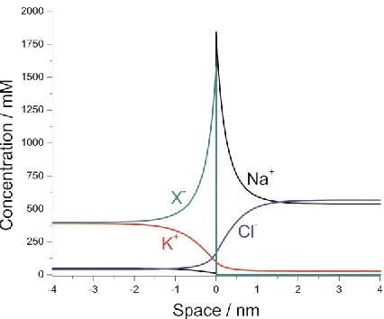
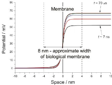
Figure 2 shows the long time concentration profiles of all the species in the simulated system. The time evolution of the potential profile of a simulated system using the conditions expressed in Table 2 is shown in Figure 3. The simulated limiting potential difference over all space, ΔφMem, is

-66.9 mV, 99% of which is contained within approximately 4 nm (approximately half the width of a biological membrane[11]) of the infinitesimal membrane. This is achieved in approximately 10 μs. Note that the distribution is asymmetric.

Figure 3. Potential profiles at t ≈ 7 ns, 70 ns, 700 ns, 7 μs and 70 μs.

The Goldman equation for a membrane of finite thickness using the same initial conditions (with PK = PCl) gives a value of ΔφMem = −67.29 mV, which is in reasonable agreement with the

simulated result, despite the difference in the models. While the potential difference extends some distance from the membrane, it does remain largely local to the membrane area and persists at a constant value up to long time.

4. CONCLUSION

We have demonstrated that for a membrane system that has no arbitrary restrictions on its spatial extent, the potential difference may extend into solution a distance which is comparable to the thickness of a typical biological membrane. For a simulation modelling the squid giant axon, the limiting potential difference was achieved in approximately 40 μs and extended approximately 2 nm from the membrane in either direction.

ACKNOWLEDGEMENT

E.J.F.D. thanks St John’s College, Oxford, for support via a graduate scholarship.

References

1. D. E. Goldman, J. Gen. Physiol. 27 (1943) 37.

2. J. W. Perram and P. J. Stiles, Phys. Chem. Chem. Phys. 8 (2006) 4200.

3. K. R. Ward, E. J. F. Dickinson and R. G. Compton, J. Phys. Chem. B 114 (2010) 10763. 4. I.Streeter, and R. G. Compton, J. Phys. Chem. C 112 (2008) 13716.

5. E. J. F. Dickinson, L. Freitag and R. G. Compton, J. Phys. Chem. B 114 (2010) 187. 6. K. R. Ward, E. J. F. Dickinson and R. G. Compton, J. Phys. Chem. B 114 (2010) 4521. 7. A.Einstein, Ann. Phys. 17 (1905) 549.

8. A.L. Hodgkin and B. Katz, J. Physiol. 108 (1949) 37.

10.R. R. Walters, J. F. Graham, R. M. Moore and D. J. Anderson, Anal. Biochem. 140 (1984) 190. 11.L. Stryer, J. M. Berg and J. L. Tymoczko, Biochemistry, 6th Ed., W. H. Freeman & Co., New

York, 2006.