On Easiest Functions for Mutation Operators in Bio-Inspired Optimisation

(1)

DOI 10.1007/s00453-016-0201-4

On Easiest Functions for Mutation Operators in

Bio-Inspired Optimisation

Dogan Corus2 · Jun He1 · Thomas Jansen1 · Pietro S. Oliveto2 · Dirk Sudholt2 ·

Christine Zarges1

Received: 30 September 2015 / Accepted: 9 August 2016

Abstract Understanding which function classes are easy and which are hard for a given algorithm is a fundamental question for the analysis and design of bio-inspired search heuristics. A natural starting point is to consider the easiest and hardest functions for an algorithm. For the (1+1) EA using standard bit mutation (SBM) it is well known

thatOneMaxis an easiest function with unique optimum whileTrapis a hardest.

In this paper we extend the analysis of easiest function classes to the contiguous somatic hypermutation (CHM) operator used in artificial immune systems. We define a functionMinBlocksand prove that it is an easiest function for the (1+1) EA using

CHM, presenting both a runtime and a fixed budget analysis. SinceMinBlocksis,

up to a factor of 2, a hardest function for standard bit mutations, we consider the effects of combining both operators into a hybrid algorithm. We rigorously prove that by combining the advantages ofkoperators, several hybrid algorithmic schemes have optimal asymptotic performance on the easiest functions for each individual operator. In particular, the hybrid algorithms using CHM and SBM have optimal asymptotic performance on bothOneMaxandMinBlocks. We then investigate easiest functions for hybrid schemes and show that an easiest function for a hybrid algorithm is not just a trivial weighted combination of the respective easiest functions for each operator.

Keywords Running time analysis·Theory·Hybridisation·Evolutionary algorithms·Artificial immune systems

B

Christine Zarges [email protected]

(2)

1 Introduction

Over the past years many bio-inspired search heuristics such as evolutionary algo-rithms, swarm intelligence algoalgo-rithms, or artificial immune systems, have been developed and successfully applied to various optimisation problems. These heuristics have different strengths and weaknesses in coping with different fitness landscapes. Determining which heuristic is the best choice for a given problem is a fundamental and important question.

We use rigorous theoretical analyses to contribute to a better understanding of bio-inspired algorithms. A natural step is to investigate which functions are easy and which are hard for a given algorithm as this yields fundamental insights into their working principles, particularly with respect to their strengths and weaknesses.

Knowing how well an algorithm performs on its easiest and hardest functions, with regards to the expected optimisation time, provides general insights, as the expected optimisation time ofeveryfunction will be no less than that of an easiest function and no more than that of a hardest function. With respect to applications, such research may also provide guidelines for the design of benchmarks for experimental studies [10].

For a simple elitist (1+1) evolutionary algorithm (EA) using only standard bit mutations (SBM) Doerr, Johannsen, and Winzen showed thatOneMax, a function

simply counting the number of ones in a bit string, is the easiest problem among all functions with a single global optimum [8]. This statement generalises to the class of all evolutionary algorithms that only use standard bit mutation for variation [33] as well as higher mutation rates and stochastic dominance [37]. On the other hand, He et al. [10] showed that the highly deceptive functionTrapis the hardest function for the (1+1) EA.

In this work we consider typical mutation operators in artificial immune systems where no such results are available. Mutation operators in artificial immune systems [6] usually come with much larger mutation rates than mutation operators in evolution-ary algorithms. One such example is the somatic contiguous hypermutation (CHM) operator from the B-cell algorithm (BCA) [23], where large contiguous blocks of a bit string are flipped simultaneously. Previous theoretical work on comparing SBM and CHM has contributed to the understanding of their benefits and drawbacks in the context of its runtime on different problems [14,17,18], the expected solution quality after a pre-defined number of steps [21], and in dynamic environments [22]. It is easy to see that hardest functions for CHM with respect to expected optimisation times are those where the algorithm gets trapped with positive probability such that the opti-misation time is not finite, e. g., if there exists a second best search point for which all direct mutations to the optimum involve non-contiguous bits [17]. However, it is an open problem and the next step forward to determine what kind of functions are easiest for this type of mutation operator.

(3)

Hybridisations such as hyper-heuristics [30] and memetic algorithms [27] have become very popular over recent years. But despite their practical success their theoret-ical analysis is still in its infancy, noteworthy examples being the work in [1,24,32,34]. However, nothing is known about easiest or hardest functions for such algorithms.

The goals of this paper are twofold. We first want to understand what functions are easy for CHM and investigate the performance of CHM and SBM on these functions. Afterwards we consider hybridisations of SBM and CHM and easiest functions for such algorithms. We first use the method by He et al. [10], explained in Sect.3, to derive an easiest function for CHM which we callMinBlocks. In Sect.4we present an analysis of the optimisation time as well as a fixed budget analysis for CHM on

MinBlocks. We then show that SBM alone is not able to optimise the constructed

function and that a hybridisation of SBM and CHM can have significant advantages (Sect. 5.1). Finally, we investigate properties of easiest functions for such hybrid algorithms (Sect.5.3).

This journal paper extends a preliminary conference paper [4] in several ways. Firstly, in Sect.3it is discussed how the framework for determining easiest and hardest functions is not restricted to (1+1)-style algorithms, but is general enough to apply for a much larger class of algorithms including (1+λ) EAs [13] and the recently popular (1+(λ, λ)) GA using mutation and crossover [7]. Secondly, the analysis of the advantages of hybridisation in Sect.5.1has been considerably extended. Rather than just giving an example of a hybrid algorithm using one out of two operators at each step with constant probability, the analysis has been generalised to allow different hybridisation schemes and an arbitrary numberkof operators. Finally, in Sect.5.2an experimental analysis is presented to shed light on the performance of the algorithms for fitness functions that depend both on the number of ones (i.e.,OneMax) and the number of blocks (MinBlocks) in the bit string.

2 Preliminaries

We are interested in all strictly elitist (1+1) algorithms with time independent variation operators which we formally define in Algorithm1for maximisation problems. We refer to any algorithm belonging to this scheme as a (1+1) A. This generalised algo-rithmic scheme keeps a single solutionxas a population and creates a single offspring at every generation. The new offspring is accepted if it is strictly fitter than the parent. The algorithm outputs the best found solution once a termination condition is satisfied. Since in this paper we are interested in the expected number of steps required by the algorithm to find an optimal solution, we will assume that the algorithm runs forever and we will callruntimethe number of fitness function evaluations performed before the first point in time when the optimum is found.

(4)

Algorithm 1(1+1) A 1:input: fitness functionf;

2: generate an initial solutionxuniformly at random; 3:whiletermination condition is not satisfieddo 4: y←is mutated from parentx;

5: if f(y) > f(x) then

6: letx←y; 7: end if 8:end while 9:output:x.

variation operator flips each bit independently with probability 1/n. SBM is formally defined in Algorithm2.

Algorithm 2Standard Bit Mutation (SBM) fori:=0 to n−1do

with probability 1/nsetx[i]:=1−x[i]; end for

We will refer to the (1+1)Athat uses SBM as the (1+1) EA, the most widely studied evolutionary algorithm.

The other variation operator of interest is the contiguous hypermutation operator (CHM), which mutates a bit string by picking a bit position and flipping a random number of bits that follow it (in a wrapping around fashion) each with probabilityr. As done in previous work (see, e. g., [17]), we only consider the extreme case here and setr =1. CHM is formally defined in Algorithm3.

Algorithm 3Somatic Contiguous Hypermutation (CHM) selectp∈ {0,1, ...,n−1}uniformly at random;

selectl∈ {0,1, ...,n}uniformly at random; fori:=0 to l−1do

with probabilityrsetx[(p+i) modn]:=1−x[(p+i) modn]; end for

We will refer to the (1+1)Athat uses a CHM operator as (1+1) CHM.

Note that Algorithm 1 uses strict selection, i. e. only strict improvements are accepted. For most of our theoretical results we also consider a variant of Algorithm1

with non-strict selection, where the acceptance condition “f(y) > f(x)” is replaced by “f(y)≥ f(x)”.

3 Easiest and Hardest Functions

(5)

arg max

x∈S

f(x), (1)

whereSis a finite set.

LetT(A, f,x)denote the expected number of function evaluations for the (1+1)A to find an optimal solution for the first time when starting atx(expected hitting time). In the following we only consider algorithms and functions that lead to a finite expected hitting time.

Definition 1 [10, Definition 1] Given a (1+1) A for maximising a class of fitness functions with the same optima (denoted byF), a function f in the class is said to be aneasiestfunction for the (1+1) AifT(A, f,x)≤ T(A,g,x)for everyg ∈F and everyx∈S. A function f in the class is said to be ahardestfunction for the (1+1) A ifT(A,f,x)≥T(A,g,x)for everyg∈Fand everyx∈S.

The above definition of easiest and hardest functions is based on a point-by-point comparison of the runtime of the EA on two fitness functions. The criteria stated in the following Lemmas4and5for determining whether a fitness function is an easiest or hardest function for a (1+1) Awere originally given in [10]. The main proof idea in [10] is to apply additive drift theorems [11], taking the expected hitting time as drift function (distance to the target state). We state these drift theorems as Theorem2, referring to the presentation of Lehre and Witt [25], who provided a self-contained proof.

Theorem 2 (Additive Drift [11,25])Let(Xt)t_≥0be a stochastic process over some bounded state space S⊆R+₀, and let T be the first hitting time of state 0. Assume that E(T | X0) <∞. Then:

(i) If E(Xt−Xt+1| X0, . . . ,Xt;Xt >0)≥δuthen E(T | X0)≤ X0/δu.

(ii) If E(Xt−Xt+1| X0, . . . ,Xt)≤δthen E(T | X0)≥ X0/δ.

Before presenting those criteria, we state and prove the following helper lemma. It is stated as Lemma 3 in [10] without proof.

Lemma 3 If the expected time T(A, f,x) is used as the drift function, then the expected drift1_is_Δ

f(x)=1for all non-optimal search points x.

Proof Let P(x,y)denote the probability that the search point yis adopted as the current search point at the end of an iteration of the (1+1) A with current search pointx. Since

y

P(x,y)=1,

T(A,f,x)=

y

P(x,y)T(A, f,x).

1 _{In drift analysis, a drift function is a non-negative function}_d₍_x₎_{such that}_d₍_x₎₌_{0 for an optimal point}

(6)

For all non-optimal search pointsx, the (1+1) A will spend one iteration and then continue from the search point reached during this transition, hence

T(A,f,x)=1+

y

P(x,y)T(A, f,y).

Together, we have

y

P(x,y)T(A, f,x)−

y

P(x,y)T(A, f,y)=1

⇔

y

P(x,y)T(A,f,x)−T(A, f,y)=1

⇔

y

P(x,y)d(x)−d(y)=1.

That isΔf(x)=1 for all non-optimal search pointsx.

First, we have the following criterion of determining whether a fitness function is an easiest function for a (1+1)A. The two lemmas below extend Theorem 1 and Theorem 2 in [10], respectively, as they are applicable to both strict elitist selection (that is, the parentxis replaced by the childyif f(y) > f(x)) and non-strict elitist selection (that is, the parentxis replaced by the childyif f(y)≥ f(x)). The framework in [10] was restricted to strict selection.

Lemma 4 Given a (1+1) A with elitist selection (either strict or non-strict) and a class of fitness functions with the same optima, if the followingmonotonically decreasing conditionholds,

– for any two points x and y, if T(A,f,x) <T(A, f,y), then f(x) > f(y),

then f is an easiest function in this class.

Proof Letg(x)be any fitness function with the same optima as f(x). Choose the runtimeT(A, f,x)as the drift function:d(x)=T(A, f,x).

When maximising f(x), according to Lemma3, for any non-optimal pointxthe driftΔf(x)=1.In the following we prove that the driftΔg(x)≤Δf(x)=1.

Let Pf(x,y)and Pg(x,y)denote the probability of mutatingx into y(which is

independent of the function f org) and thenybeing accepted (which is dependent on f org) when optimising f andg, respectively. We separately consider the negative driftΔ−_f(x)=_y_:_d₍_x_)<_d₍_y₎Pf(x,y)(d(x)−d(y))and the positive driftΔ+_f(x)=

y:d(x)>d(y)Pf(x,y)(d(x)−d(y)) and note that Δf(x) = Δ+_f(x)+Δ−_f(x) as

transitions withd(x)=d(y)do not contribute toΔf. The same notation is used for Δg.

(7)

yis never accepted and thenΔ−_f(x) = 0.But for g(x), the negative drift is not positive. Thus we have

Δ−g(x)≤0=Δ−f(x). (2)

Positive drift: letxandybe two points such thatd(x) >d(y). Ifyis an optimum, then naturally f(x) < f(y). Ifyis not an optimum, then according to the monotonically decreasing condition, f(x) < f(y).

LetP[m](x,y)denote the probability of mutatingxintoy(which is independent of f org).

For f(x), since f(x) < f(y), y is always accepted and then Pf(x,y) =

P[m](x,y).But for g(x), since g(x) might be larger, smaller than or equal to g(y),Pg(x,y)≤P[m](x,y). Hence

Δ+g(x)=

y:d(x)>d(y)

Pg(x,y)(d(x)−d(y))

≤

y:d(x)>d(y)

Pf(x,y)(d(x)−d(y))=Δ+f(x).

Considering both negative drift and positive drift, we get Δg(x)≤Δf(x)=1.

Since Δg(x) ≤ 1 for all x, according to Theorem 2, the expected runtime is

T(A,g,x)≥d(x)=T(A,f,x)and the theorem statement is derived.

In a similar way, we have the following criterion of determining whether a fitness function is a hardest function for a (1+1) A, assuming that all expected optimisa-tion times are finite2. The monotonically decreasing condition in the above lemma is replaced by the monotonically increasing condition.

Lemma 5 Given a (1+1) A with elitist selection (either strict or non-strict) and a class of fitness functions with the same optima, if the followingmonotonically increasing conditionholds,

– for any two non-optimal points x and y, if T(A, f,x) <T(A, f,y), then f(x) < f(y),

then f is a hardest function in this class.

Proof Letg(x)be any fitness function with the same optima as f(x). Choose the runtimeT(A, f,x)as the drift function:d(x)=T(A, f,x).

For f(x), according to Lemma3, for any non-optimal pointxthe driftΔf(x)=1.

Forg(x), we prove that the driftΔg(x)≥Δf(x)=1, using the notation for positive

and negative drift from the proof of Lemma4.

2 _{Hardest functions are formally only defined for functions and algorithms with finite expected optimisation}

(8)

Positive drift: letxandybe two points such thatd(x) >d(y). LetP[m](x,y)denote the probability of mutatingxintoy(which is independent of f org). For f(x), if yis an optimum point, then the probability thatxis mutated intoyand is accepted, Pf(x,y), is equal toP[m](x,y). Similarly forg(x),Pg(x,y)=P[m](x,y)ifyis

an optimum point. Ify is not an optimum point, according to the monotonically increasing condition, f(x) > f(y). For f(x), since f(x) > f(y), the probability Pf(x,y)=0. But for g(x), sinceg(x)might be larger, smaller than or equal to

g(y), Pg(x,y) ≥ 0. Thus we have Pg(x,y) ≥ Pf(x,y)for all(x,y)such that

d(x) >d(y). Therefore, the positive drifts forgand f satisfy

Δ+g(x)=

y:d(x)>d(y)

Pg(x,y)(d(x)−d(y))

≥

y_:d₍x_)>d₍y₎

Pf(x,y)(d(x)−d(y))=Δ+_f(x).

Negative drift: letxandybe two points such thatd(x) <d(y). Then according to the monotonically increasing condition, f(x) < f(y).

For f(x), since f(x) < f(y), y is always accepted and then Pf(x,y) =

P[m](x,y).But for g(x), since g(x) might be larger, smaller than or equal to g(y),Pg(x,y)≤P[m](x,y). Hence

Δ−g(x)=

y:d(x)<d(y)

Pg(x,y)(d(x)−d(y))

≥

y:d(x)<d(y)

Pf(x,y)(d(x)−d(y))=Δ−f(x).

Considering both negative drift and positive drift, we get Δg(x)≥Δf(x)=1.

Since Δg(x) ≥ 1 for all x, according to Theorem 2, the expected runtime is

T(A,g,x)≤d(x)=T(A,f,x)and the theorem statement is derived.

(9)

example for such an algorithm is the so-called (1+(λ,λ)) GA [7], the first realistic evolutionary algorithm to provably beat theΩ (nlogn)lower bound onOneMax. We see that the framework is much more general and useful than it may appear at first sight. We have already mentioned that we consider functions where an algorithm does not have finite expected optimisation time to be harder than those with finite expected optimisation times. It is well known that CHM (Algorithm3) can be trapped in local optima when the parameterr is set to r = 1 [2] (see [17, p. 521] for a concrete example demonstrating this effect). Settingr=1, however, reveals properties of the hypermutation operator in the clearest way and this is the reason we stick to this choice (compare [17]). This implies that analysing hardest functions for (1+1) CHM does not make much sense because it is easy to find functions where there is a positive probability that the algorithm gets stuck in a local optimum so that, consequently, the expected optimisation time is not finite. One could consider different measures of hardness for this situation, e. g., considering the conditional expected optimisation time given that a global optimum is found or, alternatively, considering the probability not to find a global optimum. This, however, is beyond the scope of this article.

4 Contiguous Hypermutations on an Easiest Function with a Unique

Global Optimum

We are now ready to derive an easiest function with a unique global optimum for contiguous hypermutations and analyse the performance of the (1+1) CHM on this function.

4.1 Notation and Definition

We usex=x[0]x[1] · · ·x[n−1] ∈ {0,1}nas notation for bit strings of lengthn. For a,b ∈ {0,1, . . . ,n−1}we denote byx[a. . .b]the concatenation ofx[a],x[(a+ 1)modn],x[(a+2)modn], …,x[(a+i)modn]wherei is the smallest number from{0,1, . . . ,n−1}with(a+i)modn=b. We denote by|x[a. . .b]|the number of bits inx[a. . .b], i. e., its length. We say thatx ∈ {0,1}ncontains a 1-block from atobifx[a. . .b] =1|x[a...b]|andx[(a−1)modn] =x[(b+1)modn] =0 hold. Analogously we may speak of a 0-block fromatob. Note that bit strings need to contain at least one 0-bit and at least one 1-bit to contain a 0-block or a 1-block. It is easy to see that eachx∈ {0,1}n\ {0n,1n}contains an equal number of 0-blocks and 1-blocks.

Definition 6 We define an easiest function with unique global optimum for contiguous hypermutations by defining a partition L0 ˙∪ L1 ˙∪ L2 ˙∪ · · · ˙∪ Ll = {0,1}n and

assigning fitness values accordingly. We call the function MinBlocks and define

MinBlocks(x)=l−iforx∈Li. We definel= n/2+1 and level setsL0= {1n},

L1 = {0n}andLi = {x ∈ {0,1}n | x containsi −1 different 1-blocks}for each

i ∈ {2,3, . . . ,l}.

(10)

We defer the proof thatMinBlocksis indeed an easiest function for (1+1) CHM to the next section (Theorem8) in order to make use of arguments from the analysis of the expected optimisation time performed there.

4.2 Expected Optimisation Time

We analyse the expected optimisation time of the (1+1) CHM onMinBlocks, i. e.,

the expected number of function evaluations executed until the global optimum is reached [12]. To facilitate our analysis, we start with an analysis of the expected optimisation time starting from a bit string from a particular level set which will in turn allow us to prove thatMinBlocksis an easiest function for (1+1) CHM. We will then continue with the overall upper and lower bounds for the optimisation time.

Lemma 7 We consider (1+1) CHM with strict or non-strict selection onMinBlocks

as defined in Definition6. For i∈ {0,1, . . . ,l}(where l+1is the number of sets in the partition from Definition6)let Ti denote the random number of steps needed to

reach the unique global optimum1nwhen started in a bit string from Li. The expected

numbers of steps are E(T0)=0, E(T1)=n+1, E(T2)=(n+1)2/2and

E(Ti)=

n(n+1)

(2i−2)(2i−3)+E(Ti−1) for all i∈ {3,4, . . . ,l}.

Proof The statement about E(T0)is trivial. For E(T1)it suffices to observe that any hypermutation which chooses as mutation lengthnleads from 0nto the unique global optimum 1n. Such a mutation has probability 1/(n+1)which implies E(T1)=n+1. For E(T2)we observe that for eachx ∈ L2 there are two mutations which lead to L0∪L1, one leading toL0and the other leading toL1. SinceL0andL1are reached with equal probability 1/2 we have E(T2)=n(n+1)/2+E(T1)/2=(n+1)2_/_{2. For E}₍_T

i)

withi >2 we observe that only mutations that reduce the number of 1-blocks can lead to someLjwithj <i. It is easy to see that, the number of 1-blocks can only be reduced

by 1 in one contiguous hypermutation. In order to achieve that a mutation must start at the first bit of a block (either a 0-block or a 1-block) and end at the last bit of a block (either a 0-block or a 1-block) but this block cannot be the one just before the block containing the first flipped bit (otherwise the length of the mutation isn, the bit string is inverted and the number of 1-blocks remains unchanged). Thus, if there are jblocks in the bit string, the number of such mutations equals j(j−1). Forx∈ Lithe number

of 1-blocks equalsi−1 and therefore the number of blocks equals 2i−2 so that there are(2i−2)(2i−3)such mutations. Thus, the expected time to leaveLiequalsn(n+

1)/((2i−2)(2i−3))and E(Ti)=n(n+1)/((2i−2)(2i−3))+E(Ti₋1)follows. The expected runtimes provided in Lemma7allow us to verify whetherMinBlocks

satisfies the criteria set by Lemma4. The following theorem establishesMinBlocks

as an easiest function for (1+1) CHM.

(11)

Proof The theorem follows from Lemma 7, the definition of MinBlocks, and Lemma4. According to Definition6, for alli ∈ {1,2, . . . ,n/2}the fitness value of solutions in subset Li is strictly less than the fitness value of solutions inLi−1.

Therefore, a solution x has a better MinBlocks value than a solution y, if and

only if x and y belong to two distinct subsets Li and Lj respectively such that

i < j. Note that in Lemma7 the expected runtime of the (1+1) CHM initialised with a solution from Li, E(Ti), satisfies E(Ti) >E(Ti−1)for alli and thusi < j implies E(Ti) < E

Tj

. Therefore,MinBlocks(x) > MinBlocks(y)if and only

if the expected runtimes of (1+1) CHM starting from solutions x and y satisfy T(A, f,x) = E(Ti) < E

Tj

= T(A,f,y). According to Lemma4, the above two way implication makesMinBlocksan easiest function for the (1+1) CHM.

We continue our analysis of the expected optimisation time. Note that the following bound asymptotically matches the lower bound ofΩn2for contiguous hypermuta-tions and funchypermuta-tions with a unique global optimum proven by Jansen and Zarges [17].

Theorem 9 Let T denote the expected optimisation time of the (1+1) CHM with strict or non-strict selection onMinBlocks. E(T)=ln(2)n2±O(n)holds.

Proof Considerx ∈ {0,1}nselected uniformly at random. For eachi∈{0,1, . . . ,n−1} we have that a block ends atx[i]ifx[i] =x[(i+1)modn]holds. Thus,x[i]is the end of a block with probability 1/2 and we see that the expected number of blocks equals n/2. Let I denote the number of blocks. An application of Chernoff bounds yields that for any constantεwith 0< ε <1 we have Pr(I ≥(1−ε)n/2)=1−e−Ω(n).

We know that E(T | I =2(i−1))=E(Ti)holds and have

E(Ti)=

n(n+1)

(2i−2)(2i−3)+E(Ti−1)

= ₍ n(n+1)

2i−2)(2i−3)+

n(n+1)

(2(i−1)−2)(2(i−1)−3)+E(Ti−2)

= · · · =E(T2)+n(n+1)

i−3

j=0

1

(2(i−j)−2)(2(i− j)−3)

=E(T2)+n(n+1)

i−3

j₌0

1 2j+3+

1 2j+4 −

1 j+2

=E(T2)+n(n+1)

⎛ ⎝ ⎛

⎝2i−2

j=3 1

j

⎞

⎠₋

⎛

⎝i−1

j=2 1

j

⎞ ⎠ ⎞ ⎠

=E(T2)+n(n+1)

H2i−2−Hi−1− 1 2

whereHjdenotes thejthharmonic number. UsingHj =ln(j)+γ+1/(2j)−o(1/j)

(12)

E(T | I =2(i−1))= (n+1) 2

2 +n(n+1)

ln(2)−1 2

−O

n2/i

=ln(2)n2+O(n)−O

n2/i

.

For the lower bound on E(T)we usei = (n/8)+1 (and have Pr(I ≥n/4)= 1−e−Ω(n), of course) and obtain

E(T)≥Pr(I ≥n/4)·E(T |I ≥n/4)

=1−e−Ω(n)

·ln(2)n2+O(n)−O(n)

=ln(2)n2±O(n)

as claimed.

For the upper bound on E(T)we have

E(T)≤ETn/2

=ln(2)n2+O(n)−O(n)=ln(2)n2±O(n) as claimed.

4.3 Fixed Budget Analysis

It has been pointed out that the notion of optimisation time does not always capture the nature of how randomised search heuristics are applied in practice. As a result, fixed budget analysis has been introduced as an alternative theoretical perspective [19,20]. Letxt denote the current population aftertrounds of contiguous hypermutation and

selection. In fixed budget analysis we want to analyse E(f(xt))for allt ≤ E(T)

where E(T)is the expected optimisation time. We do this here for MinBlocksto

give a more complete picture about the performance of the (1+1) CHM. Note that a comparison of the (1+1) EA and the (1+1) CHM under the fixed budget perspective has previously been performed for some example functions [21].

We begin with a statement about the expected function value of a uniform random solution, reflecting the way (1+1) A algorithms are initialised, and prove that it is roughly(n−2)/4±1/2.

Theorem 10 Let x0∈ {0,1}nbe selected uniformly at random and f :=MinBlocks

from Definition6. For the initial function value E(f(x0)) = n/2 −(n/4)+2−n holds.

Proof We know from the analysis of the expected optimisation time in Sect.4.2that the expected number of blocks inx0equalsn/2. Letz(x0)denote the number of 0-blocks inx0and remember that the number of 0-blocks is half the number of blocks. This implies E(z(x0))=n/4.

(13)

We have

E(f(x0))=

x∈{0,1}n

f(x) 2n =

x∈{0,1}n_\{₁n_}

l−1−z(x) 2n

+ l

2n

=

x∈{0,1}n_\{₁n_}

l−1−z(x) 2n

+ l

2n +

l−1−z(1n₎

2n −

l−1−z(1n₎

2n

=

x∈{0,1}n

l−1−z(x) 2n

+ l

2n −

l−1−z(1n₎

2n

=

x∈{0,1}n

l−1−z(x) 2n

+ 1

2n =E(l−1−z(x0))+

1 2n

=l−1−E(z(x0))+2−n =l−1−(n/4)+2−n

and obtain the claimed bound by remembering thatl= n/2 +1 holds.

We now give upper and lower bounds on the expected function value aftertiterations of the (1+1) CHM.

Theorem 11 Let xt ∈ {0,1}n denote the current search point after random

initiali-sation and t rounds of contiguous hypermutation and strict or non-strict selection on

f :=MinBlocks. The following bounds hold for the expected function value after t

steps E(f(xt)).

lower boundE(f(x0))+

_n

2

+1−E(f(x0)) 1−

1− 2 n(n+1)

t

≤n

2

+1−

_n

2

+1−E(f(x0))

·

1− 3 n(n+1)

t

≤E(f(xt))

upper boundE(f(xt))

≤

n/2

z=1

n/2 z

2−n/2· n 2 −z

+1−

1− 1 n+1

t

+

z+1

d=2

1−

1−(2d−2)(2d−3) n(n+1)

t

+n·2−n+1

Proof The function value can increase at mostn/2 +1−ztimes if the initial func-tion value isz since the maximal function value isn/2 +1. For an upper bound we consider the actual probabilities for increasing the function value which equal

(14)

these yields an upper bound since it pretends that for each leveltsteps are available to create an increasing step whereas in reality decreasing the number of 0-blocks fromd tod−1 is only possible after it has been decreased todfromd+1 before. Since initial-isation in 0n_{or 1}n_{has probability 2}−n+1_{the contribution of these cases is}_O₍_n_/₂n₎_.

LetZdenote the random number of 0-blocks in the initial bit string. We obtain

E(f(xt))≤ n/2

z=1

Pr(Z =z)·

(l−(z+1))

+1−

1− 1 n+1

t

+

z₊1

d=2

1−

1−(2d−2)(2d−3) n(n+1)

t

+l·2−n+1

using the law of total probability. We obtain an upper bound by noting thatZis binomi-ally distributed with parametersn/2 and 1/2, and by remembering thatl = n/2 +1 holds.

For the smaller of the two lower bounds we replace the actual probabilities by the smallest probability for an increase in function value which equals 2/(n(n+1)). We can improve on this weak lower bound slightly by using a technique called multi-plicative fixed budget drift as recently introduced by Lengler and Spooner [26]. For a lower bound we need a lower bound on the expected change in function value in one generation given the current function value. If the current bit string contains i bits, we know that the expected change equals (2i −2)(3i −2)/(n(n +1)) > 3i2/(n(n+1)) > 3i/(n(n +1))where the last inequality is made because Theo-rem 1 in [26] requires a statement about this drift that is linear. Using this we obtain

n/2 +1−(n/2 +1−E(f(x0)))·(1−3/(n(n+1)))t as lower bound on the expected function value aftertsteps.

To obtain actual lower and upper bounds we use the lower and upper bounds for the initial expected function value from Theorem10. While the bounds from Theorem11

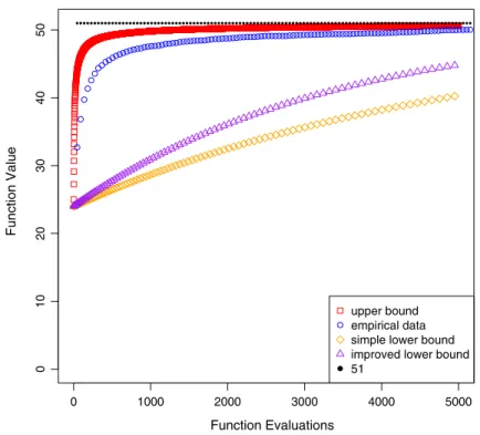
are not simple and in particular the upper bound is not even a closed form, we can easily evaluate them numerically for reasonable values of n. In Fig. 1 we display them forn =100 together with the maximal function value 51 and empirical results averaged over 100 runs. We see that while the upper bound yields reasonable results both lower bounds are rather weak.

5 Hybridising Operators

A popular approach in areas such as memetic algorithms [27] or hyper-heuristics [30] is to combine several operators in one algorithm. There are many ways of hybridising algorithms – here, we consider four different schemes of hybridisation that combinek operators. Given several (1+1)As,A1,· · · ,Ak, the different hybridisations considered

are:

(15)

0 1000 2000 3000 4000 5000

0

1

02

03

04

05

0

Function Evaluations

Function Value

upper bound empirical data simple lower bound improved lower bound 51

Fig. 1 Average function values for the (1+1) CHM on an easiest function for the (1+1) CHM with unique global optimum forn=100 after a given number of function evaluations, averaged over 100 runs, together with the theoretical bounds from Theorem11. The empirical data was produced with a (1+1) CHM with strict selection

(1+1) HA-chained: executing a chain of operators, where operators are applied prob-abilistically according to a given probability vectorp=(p1, . . . ,pk)(Algorithm5,

note that pdoes not have to be a probability distribution),

(1+k) HA: executing all operators in parallel and picking the best among the resulting solutions (Algorithm6), and

k×(1+1) HA: executing all operators sequentially, resulting in a chained sequence of operations, with selection after each operator (Algorithm7).

The (1+1) HA-chained is probably the most commonly used method in hybrid algo-rithms. For instance, most Genetic Algorithms fall into this category since they use a probabilitypcthat crossover is applied before mutation. The (1+1) HA is commonly

(16)

idea also appears in simple island models with heterogeneous islands, that is, each island consists of one individual and uses a different variation operator. A real-world example of where such a strategy is used (albeit with populations and added complex-ity) is the Wegener system, a popular and effective algorithm in search-based software testing, where different islands use standard bit mutations with different mutation rates [36]. Thek×(1+1) HA is interesting as it has some resemblance to the recently introduced (1+(λ,λ)) GA, since both use selection between the application of the oper-ators. However, the (1+(λ,λ)) GA does not fall exactly within thek×(1+1) HA scheme. In the former, if the final solution is worse than the initial one in the sequence, then the initial solution is accepted for the next generation. On the other hand, thek×(1+1) HA always accepts the last improving solution in the sequence.

Note that (1+1) HA-chained andk×(1+1) HA differ in the use of selection: the latter applies selection after each operator, whereas the former only applies selection at the end of the generation. One generation of (1+k) HA may be regarded as a derandomised version of (1+1) HA(1/k, . . . ,1/k)run forkgenerations. In the former all operators are executed once, whereas in the latter algorithm all operators are executed oncein expectation. The latter also admits non-uniform probabilities.

Algorithm 4Hybrid algorithm (1+1) HA(p)(probabilistic choice of operator) 1:input: fitness functionf;

2: generate a solutionx;

3:while the maximum value of fis not found do 4: chooseAiwith probabilitypi;

5: apply one iteration (mutation and selection) ofAito generatey; 6: updatexwithyif f(y) > f(x);

7:end while

8:output: the maximal value of f.

Algorithm 5Hybrid algorithm (1+1) HA-chained(p)(probabilistic chain) 1:input: fitness functionf;

3:while the maximum value of fis not found do 4: lety:=x;

5: fori=1, . . . ,kdo

6: with probabilitypiupdateyby applying one iteration ofAiwithout selection; 7: end for

8: updatexwithyif f(y) > f(x); 9:end while

Algorithm 6Hybrid algorithm (1+k) HA (parallel operations) 1:input: fitness functionf;

3:while the maximum value of fis not found do

4: fori=1, . . . ,kdo

5: apply one iteration (mutation and selection) ofAito generateyi; 6: end for

7: updatexwith a best search point from{y1, . . . ,yk}if its fitness is larger than f(x); 8:end while

(17)

Algorithm 7Hybrid algorithmk×(1+1) HA (sequential operations) 1:input: fitness functionf;

3:while the maximum value of fis not found do

4: fori=1, . . . ,kdo

5: apply one iteration (mutation and selection) ofAito generatey; 6: updatexwithyif f(y) > f(x);

7: end for 8:end while

The B-cell algorithm (BCA) [23] is an example of an algorithm that uses both SBM and CHM considered in this paper. More specifically, it uses a population of search points and createsλclones for each of them. It then applies standard bit mutation to a randomly selected clone for each parent search point and subsequently applies CHM to all clones. This way one offspring of each parent is subject to a sequence of two mutations, first standard bit mutation and afterwards CHM. Jansen et al. [14] proposed a variant of the BCA that only uses CHM with constant probability 0 < p < 1 (instead of p =1) and were able to show significantly improved upper bounds on the optimisation time for this algorithm on instances of the vertex cover problem. Considering the individuals that undergo both kinds of mutation (or a (1+1)-style BCA), both these variants fit within the (1+1) HA-chained model of hybridisation (Algorithm5). More precisely, for p =(p1,p2)with p1the probability to execute SBM and p2the probability to execute CHM, we have p1= p2=1 for the original BCA and constant p1=1 and 0<p2<1 for the modified BCA in [14]. We remark that the improved results in [14] in fact hold as long as p1=Ω (1).

In the following subsection we will first consider the general hybrid algorithmic framework and then specialise the results to the combination of CHM and SBM.

5.1 The Advantage of Hybridisation

The easiest functions for SBM and CHM areOneMaxandMinBlocks, respectively. Before analysing hybrid algorithms using both operators, it is natural to consider the effect of one operator on the easiest function for the other operator. It is well known that the (1+1) CHM needs (n2logn)expected time onOneMax[17,21].

Here we consider the expected optimisation time of the (1+1) EA onMinBlocks

and show that it is very inefficient.

Theorem 12 The expected optimisation time of the (1+1) EA with strict or non-strict selection onMinBlocksis at least nn/2.

Proof The function MinBlocks has the following property: for all search points except for 0nand 1n, the number of 0-blocks equals the number of 1-blocks. Notice that inverting all bits in a bit string turns all 0-blocks into 1-blocks and vice versa. Hence for allx∈ {/ 0n,1n}we haveMinBlocks(x)=MinBlocks(x).

(18)

x0,x1, . . . ,xT andxT ∈ {0n,1n}, we have Pr(xT =0n)=1/2. In this case the only

accepted search point is the global optimum 1n, for which all bits have to be flipped in one mutation. This has probabilityn−nand expected waiting timenn. Combined with the probability of reaching this state, the expected optimisation time is at least T +nn/2≥nn/2.

Note that the expected optimisation time of the (1+1) EA onMinBlocksis only by a factor of at most 2 smaller than the expected optimisation time of the (1+1) EA on its hardest function,Trap, which is almostnn[9].

Using multiple operators, the hope is that the advantages of each operator are com-bined. However, this is not always true: new operators can make a hybrid algorithm follow an entirely different search trajectory and lead to drastically increased optimi-sation times. This behaviour was demonstrated for memetic algorithms [31] as well as for standard bit mutations cycling between different mutation rates [15] and for population based EAs where the mutation rate of each individual depends on its rank in the population [28].

We show that such effects cannot occur when dealing with easiest functions. If f is an easiest function forAwhich is a (1+1) A, then Theorem13stated below allows to transfer an upper bound on the expected optimisation time ofAto the four hybrid algorithms.

Theorem 13 If A1, . . . ,Akare (1+1) A’s with strict or non-strict selection, starting

in x0, and f is an easiest function for Ai, then the expected hitting time of (1+1) HA(p)

on f , for a probability distribution p=(p1, . . . ,pk), is bounded from above by

1 pi ·

T(Ai,f,x0).

For any probability vector p =(p1, . . . ,pk)with pi >0and pj <1for all j =i ,

the expected hitting time of (1+1) HA-chained(p)on f is bounded from above by

1 pi·

j=i(1−pj)·

T(Ai,f,x0).

Moreover, the expected hitting time of (1+k) HA and k×(1+1) HA is bounded from above by

k·T(Ai,f,x0).

Proof We follow the analysis in [10, Section III] and perform a drift analysis, choosing the runtimeT(Ai,f,x)as the drift function:

d(x)=T(Ai, f,x).

DefineΔAj(x)=E((d(x)−d(y)))as the drift of Algorithm Aj, given thatywas

(19)

Δ(1+1)H A(x)= k

i=1

piΔAi(x).

We apply Lemma 3 in [10] to estimateΔAi. For any non-optimal pointx, letybe its

child, then the drift of algorithmAi satisfies

ΔAi(x)=E(d(x)−d(y))=1 (3)

following from the definition ofd(x)=T(Ai,f,x). We further claim that no operator

induces a negative drift. Given any two non-optimal pointsxandy, then when using strict selection, according to the monotonically decreasing condition d(x) < d(y) implies f(x) > f(y). By contraposition, we get

f(y)≥ f(x)⇒d(y)≤d(x). (4)

When using non-strict selection, the strictly monotonically decreasing condition implies f(y) ≥ f(x) ⇔ d(y) ≤ d(x), which implies (4) as well. Since all algo-rithms A1, . . . ,Ak adopt elitist selection, the distance cannot increase, regardless of

which operator is chosen. HenceΔAj(x)≥0 for all jand

Δ(1₊1₎H A(x)≥ piΔAi(x)= pi.

Using the additive drift theorem, Theorem2, the expected hitting time of (1+1) HA(p)

on f is at most

d(x0) pi =

T(Ai, f,x0)

pi .

For (1+1) HA-chained we observe that the algorithm executes only Ai and none of

the other operators with probabilitypi·

j=i(1−pj). In all other cases the distance

cannot increase (by (4)). Hence by the same arguments as above, the expected hitting time is bounded by

1 pi·

j=i(1−pj)·

T(Ai,f,x0).

The statement on(1+k)HA follows from similar arguments. Letx1, . . . ,xk be the

search points created usingA1, . . . ,Ak, respectively. Letx∗be the best amongst these,

selected for survival. Then f(x∗)≥ f(xi), and by (4),d(x∗)≤d(xi). Hence for all

non-optimalx,

Δ(1+k)H A(x)≥ΔAi(x)=1.

Additive drift from Theorem2 then yields an upper bound on the expected time of (1+k) HA ofk·T(Ai,f,x0), the factorkaccounting for executingkoperations in one

(20)

Finally, fork×(1+1) HA, letx1, . . . ,xkbe the offspring created in the sequence of

operations and note thatxkis taken over for the next generation. We have f(xi−1)≥

· · · ≥ f(x1)≥ f(x)and thusd(xi−1)≤d(x)by (4). Along withΔAi(x)=1 for all

non-optimalxand f(xk)≥ f(xi)implyingd(xk)≤d(xi), we get

Δk_×₍1₊1₎H A(x)≥ΔAi(x)=1

and an upper bound ofk·T(Ai, f,x0)as for (1+k) HA.

Using Theorem13as well as Theorem9, we get the following corollary concerning the SBM and CHM operators.

Corollary 14 Consider the hybrid algorithms (1+1) HA(p)and (1+1) HA-chained(p)

for p=(p1,p2)with constant p1,p2>0, (1+2) HA, and2×(1+1) HA, all based on a (1+1) algorithm A1using SBM and another (1+1) algorithm A2using CHM; A1 and A2both using strict or non-strict selection. Then the expected optimisation time of all these hybrids onOneMaxandMinBlocksis O(nlogn)and O(n2), respectively. All hybrid algorithms are hence able to combine the advantages of both operators on the two easiest functions for its two operators. This is particularly true for the modified (1+1)-style BCA [14] with constant 0 < p1,p2 <1 discussed at the beginning of Sect.5.

5.2 Weighted Combinations ofOneMaxand MINBLOCKS

In the previous subsection it was proven that the four different hybrid schemes (1+1) HA(p) for p = (p1,p2) with constant p1,p2 > 0, (1+1) HA-chained, (1+2) HA, and 2×(1+1) HA, using SBM and CHM as operators are all efficient

forOneMaxandMinBlocks. In particular, even though SBMs alone exhibit very

poor performance onMinBlocks, hybrid algorithms using CHM with arbitrarily low constant probability along with SBM are efficient. In this subsection we investigate the performance of the two operators on “hybrid” functions where the fitness depends on both the number of ones and the number of blocks.

To this end, we perform experiments concentrating on different instantiations of Algorithm (1+1) HA(p)forp=(p,1−p)with various values ofpand strict selection and investigate its performance on a function consisting of weighted combinations of

OneMaxandMinBlocks. To be more precise we consider the function

f_w(x)=w·OneMax(x)+(1−w)·MinBlocks(x)

(21)

for p = 1 andw = 1 (CHM on pureOneMax [17]) and n2for p = 1 and

w = 0 (CHM on pure MinBlocks, Theorem9). We are particularly interested in intermediate values of pandwand their influence on the optimisation time.

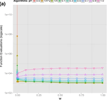
We perform 10,000 runs for each of the above pairs of settings forn =100 and depict the average optimisation times in Fig.2. Figure2a shows a comparison of the optimisation times of different resulting algorithms (1+1) HA(p,1− p)depending onwwhile Fig.2b depicts the results for different functions over the parameter pof the hybrid algorithm. Note, that for the sake of recognisability we only depict a subset of the curves in both figures while on each curve we present all available data points. We additionally perform Wilcoxon signed rank tests to assess whether the observed differences in the optimisation times are statistically significant. Fixing a value forw (Fig.2a) we perform tests for all pairs of algorithms and the 10,000 optimisation times measured for each setting. Similarly, fixing a value for p(Fig.2b) we perform tests for all pairs of functions. We perform Holm-Bonferroni correction to account for the large number of tests we execute.

We observe that for allw >0, the runtime gets smaller aspdecreases (Fig.2a). All differences are statistically significant at confidence level 0.05 with the exception of p=0 andp =1/n2_{for all values of}_w_and_p₌_0, _p₌₁_/_n2_,_p₌₁_/_n_and_p₌₀_.₁ for mostw∈ {0.1,0.2,0.3,0.4}. From Fig.2b we can also see that the (1+1) HA(p)

with constantp<0.7 appears to be faster on functions f_wwith constantw >0 (i. e., with constantOneMaxfraction) while using a largerp(i. e., performing CHM more

often) pays off forw = o(1). Differences are statistically significant at confidence level 0.05 with the exception of most results for p=0.7 andp =0.8,w=1/nand

w=1/n2for all p≤0.8,w≥0.6 for all p,w≥0.3 for all p ≥0.5, andw≤0.2 forw=0,w=1/n2andw=1/n.

We can see from the experiments in Fig.2that the casew =0 is very different from runs withw > 0. Recall thatw = 0 means that the algorithm is confronted

withMinBlocksand thatw >0 implies that we addw·OneMaxto the function

value (while, at the same time, reducing the function value byw·MinBlocks). The addition ofw·OneMaxwith an arbitrarily smallw >0 introduces a ‘search gradient’ in the fitness landscape: the algorithm is encouraged to increase the number of 1-bits by a small increase in fitness (at least as long as this trend is not counteracted by an increase in the number of blocks). The effect is most pronounced for p =0, i. e., for the (1+1) EA where the expected optimisation time is exponential forMinBlocks

and becomes manageable as soon as theOneMax-component introduces a ‘search

gradient’. In a different context, the same effect has been discussed and analysed using different example functions [16].

5.3 On the Easiest Function for Hybrid Algorithms

In the previous subsection it was shown experimentally that as soon as a smallOneMax

(22)

●

●● ● ● ● ● ● ● ● ● ● ●

●

●●

● ● ● ● ● ● ● ● ● ●

1e+02 1e+04 1e+06 1e+08 1e+10

0.00 0.25 0.50 0.75 1.00

w

Function Ev

aluations (logscale)

Algorithms: p= 0.0●1/n^2 1/n 0.1●0.3 0.5 0.7 0.9 1.0

(a)

●

●●●

●

● ● ● ●

● _● ●

1e+03 1e+04 1e+05 1e+06

0.00 0.25 0.50 0.75 1.00

p

Function Evaluations (logscale)

Functions: w= 0.0●1/n^2 1/n 0.1●0.3 0.5 0.7 0.9 1.0

(b)

Fig. 2 Results of the experiments: Average optimisation times over 10,000 independent runs for each pair ofpandwforn=100. The empirical data was produced with a (1+1) HA(p,1−p)with strict selection. aResults for different algorithms (1+1) HA(p,1−p)over values forw.bResults for different functions

(23)

algorithm (1+1) HA(1/2,1/2) using SBM and CHM, and strict selection, is more complex than a mere weighted combination fwof the two easiest functions for both operators.

He et al. [10] explain how an easiest function can be computed. We construct

EasiestHybridp, an easiest fitness function for the hybrid algorithm (1+1) HA(p,1−

p) from Corollary14by implementing their construction procedure and performing the necessary computations numerically. Clearly, this is computationally feasible only for small values ofn. Using the unique global optimum as a starting point and level L0we can compute the next level of search points with next best and equal fitness by computing for each search point which does not yet have a level the expected time needed to reachL0either directly or via a mutation to a search point that already has a level. Search points with minimal time in this round make up the next level. Note that this is actually Dijkstra’s algorithm for computing shortest paths (see, e. g., [3]). Also note that the numerical computation of the actual expected waiting times is easy since the exact transition probabilities for mutations leading from one bit string to another are all known and waiting times are all simply geometrically distributed.

The easiest function for the (1+1) CHM is composed ofn/2 +2 different fitness levels,L0, . . . ,Ln/2+1, defined by a number of 1-blocks (i. e.,L0= {1n},L1= {0n}, Li = {x∈ {0,1}n |xcontainsi−1 different 1-blocks}for eachi∈ {2, . . . ,n/2 +

1}). On the other hand, the fitness level set of the easiest function for the (1+1) EA (i. e.,

OneMax) hasn+1 different levels defined by a number of 1-bits (i. e.,Li = {x ∈

{0,1}n|xcontainsn−i1-bits}for eachi ∈ {0, . . . ,n}). IfEasiestHybridpwas a

mere weighted combination ofOneMaxandMinBlocks, its fitness levels would be

defined by a combination of a number of 1-blocks and a number of 1-bits. This would happen because individuals that have the same number of 1-bits and the same number of 1-blocks would have exactly the same fitness. Also, the product between the number of levels of the easiest functions for each operator,(n/2 +2)·(n+1), would be an upper bound on the number of levels forEasiestHybridp. In the following we

show that neither of these two considerations are true and that the fitness levels of the easiest function for the hybrid algorithm are more complicated. In particular, bit strings having in common the same number of 1-blocks and the same number of 1-bits can belong to different fitness levels ofEasiestHybridp. Rather, thelength of the

blockscomes into play to define the fitness levels even though such a feature does not define the levels of eitherOneMaxorMinBlocks.

(24)

(25)

because the level may be reached by flipping only one bit while at least three bits need to be flipped for bit strings inL8. Since the transition probabilities to the remaining levels of higher fitness are the same, the expected runtime fromL7is lower than that fromL8, explaining why the two levels are distinct (recall that, by construction, the levels are ordered according to increasing expected runtimes).

Concerning the number of different fitness levels, these increase as the problem sizenincreases. Already forn=10EasiestHybrid1/2has 78 different levels, more than the product of the number ofOneMaxandMinBlockslevels forn =10 (i. e.

66). It is indeed the increase in number of fitness levels asngrows that makes it hard to give a precise definition of theEasiestHybrid1/2 function. We leave this as an open problem for future work.

6 Conclusions

We have extended the analysis of easiest function classes from standard bit mutations to the contiguous somatic hypermutation (CHM) operator used in artificial immune systems. Albeit the recent advances in their theoretical foundations [21,29,35] no such results were available concerning artificial immune system operators. With the run-time and fixed budget analyses of the (1+1) CHM onMinBlocks, the corresponding

easiest function, we established a lower bound on the (1+1) CHM’s performance on any function. We also showed thatMinBlocksis exponentially hard for the standard

(1+1) EA, complementing the known result that the (1+1) CHM performs asymptoti-cally worse by a factor of (n)compared to the (1+1) EA onOneMax. Furthermore,

we proved that several hybrid algorithms combining the (1+1) CHM and the (1+1) EA solve bothMinBlocksandOneMaxonly at a constant factor slower than the pure algorithms.

Experimental work revealed that a fitness function consisting of a weighted com-bination of MinBlocks andOneMaxis easy to optimise for both pure operators and hybrid variants even when theOneMaxweight component is very small. Nev-ertheless, after providing the exact fitness landscape of the easiest function for the (1+1) HA(1/2,1/2),EasiestHybrid1/2 for small instance sizes, we observed that its structure is more complex than a simple weighted combination ofOneMaxand

MinBlocks. We leave constructing and analysing easiest functions for other operators

that fit the (1+1) Ascheme for future work. Similarly, the question about the easiest functions for different schemes of hybridisation remains open.

Acknowledgments The research leading to these results has received funding from the European Union Seventh Framework Programme (FP7/2007-2013) under Grant Agreement No. 618091 (SAGE) and by the EPSRC under Grant Agreement No. EP/M004252/1. We thank the anonymous reviewers of this manuscript and the previous GECCO 2015 paper for their very useful and constructive comments.

(26)

References

1. Alanazi, F., Lehre, P.K.: Runtime analysis of selection hyper-heuristics with classical learning mech-anisms. In: Proceedings of the IEEE Congress on Evolutionary Computation (CEC 2014), pp. 2515–2523. IEEE (2014)

2. Clark, E., Hone, A., Timmis, J.: A markov chain model of the B-cell algorithm. In: Proceedings of the International Conference on Artificial Immune Systems (ICARIS 2005), LNCS 3627, pp. 318–330. Springer (2005)

3. Cormen, T.H., Leiserson, C.E., Rivest, R.L., Stein, C.: Introduction to Algorithms. MIT Press, London (2001)

4. Corus, D., He, J., Jansen, T., Oliveto, P.S., Sudholt, D., Zarges, C.: On easiest functions for somatic contiguous hypermutations and standard bit mutations. In: Proceedings of the Genetic and Evolutionary Computation Conference (GECCO 2015), pp. 1399–1406. ACM (2015)

5. Cowling, P., Kendall, G., Soubeiga, E.: A hyperheuristic approach to scheduling a sales summit. In: Burke, E., Erben, W. (eds) Proceedings of the Third International Conference on Practice and Theory of Automated Timetabling (PATAT 2000), pp. 176–190. Springer (2001)

6. de Castro, L.N., Timmis, J.: Artificial Immune Systems: A New Computational Intelligence Approach. Springer, Berlin (2002)

7. Doerr, B., Doerr, C., Ebel, F.: From black-box complexity to designing new genetic algorithms. Theoret. Comput. Sci.567, 87–104 (2015)

8. Doerr, B., Johannsen, D., Winzen, C.: Drift analysis and linear functions revisited. In: Proceedings of the IEEE Congress on Evolutionary Computation (CEC 2010), pp. 1967–1974 (2010)

9. Droste, S., Jansen, T., Wegener, I.: On the analysis of the (1+1) evolutionary algorithm. Theoret. Comput. Sci.276, 51–81 (2002)

10. He, J., Chen, T., Yao, X.: On the easiest and hardest fitness functions. IEEE Trans. Evol. Comput. 19(2), 295–305 (2015)

11. He, J., Yao, X.: A study of drift analysis for estimating computation time of evolutionary algorithms. Nat. Comput.3(1), 21–35 (2004)

12. Jansen, T.: Analyzing Evolutionary Algorithms: The Computer Science Perspective. Springer, Berlin (2013)

13. Jansen, T., De Jong, K.A., Wegener, I.: On the choice of the offspring population size in evolutionary algorithms. Evol. Comput.13(4), 413–440 (2005)

14. Jansen, T., Oliveto, P.S., Zarges, C.: On the analysis of the immune-inspired B-cell algorithm for the vertex cover problem. In: Proceedings of the International Conference on Artificial Immune Systems (ICARIS 2011), LNCS 6825, pp. 117–131. Springer (2011)

15. Jansen, T., Wegener, I.: On the choice of the mutation probability for the (1+1) EA. In: Proceedings of the 6th International Conference on Parallel Problem Solving from Nature (PPSN 2000), LNCS 1917, pp. 89–98. Springer (2000)

16. Jansen, T., Wiegand, R.P.: The cooperative coevolutionary (1+1) EA. Evol. Comput.12(4), 405–434 (2004)

17. Jansen, T., Zarges, C.: Analyzing different variants of immune inspired somatic contiguous hypermu-tations. Theoret. Comput. Sci.412(6), 517–533 (2011)

18. Jansen, T., Zarges, C.: Computing longest common subsequences with the B-cell algorithm. In: Pro-ceedings of the International Conference on Artificial Immune Systems (ICARIS 2012), LNCS 7597, pp. 111–124. Springer (2012)

19. Jansen, T., Zarges, C.: Fixed budget computations: a different perspective on run time analysis. In: Proceedings of the Genetic and Evolutionary Computation Conference (GECCO 2012), pp. 1325– 1332. ACM (2012)

20. Jansen, T., Zarges, C.: Performance analysis of randomised search heuristics operating with a fixed budget. Theoret. Comput. Sci.545, 39–58 (2014)

21. Jansen, T., Zarges, C.: Reevaluating immune-inspired hypermutations using the fixed budget perspec-tive. IEEE Trans. Evol. Comput.18(5), 674–688 (2014)

22. Jansen, T., Zarges, C.: Analysis of randomised search heuristics for dynamic optimisation. Evol. Com-putation.23(4), 513–541 (2015)

(27)

24. Lehre, P.K., Özcan, E.: A runtime analysis of simple hyper-heuristics: to mix or not to mix operators. In: Proceedings of the Twelfth workshop on Foundations of Genetic Algorithms (FOGA 2013), pp. 97–104. ACM (2013)

25. Lehre, P.K., Witt, C.: General drift analysis with tail bounds. CoRR, abs/1307.2559 (2013) 26. Lengler, J., Spooner, N.: Fixed budget performance of the (1+1) EA on linear functions. In: Proceedings

of the 2015 ACM Conference on Foundations of Genetic Algorithms (FOGA 2015), pp. 52–61 (2015) 27. Neri, F., Cotta, C., Moscato, P. (eds.): Handbook of Memetic Algorithms. Springer, Berlin (2013) 28. Oliveto, P.S., Lehre, P.K., Neumann, F.: Theoretical analysis of rank-based mutation—combining

exploration and exploitation. In: Proceedings of the IEEE Congress on Evolutionary Computation (CEC 2009), pp. 1455–1462 (2009)

29. Oliveto, P.S., Sudholt, D.: On the runtime analysis of stochastic ageing mechanisms. In: Proceedings of the Genetic and Evolutionary Computation Conference (GECCO 2014), pp. 113–120. ACM (2014) 30. Ross, P.: Hyper-heuristics. In: Burke, E.K., Kendall, G. (eds.) Search Methodologies, pp. 611–638.

Springer, Berlin (2014)

31. Sudholt, D.: The impact of parametrization in memetic evolutionary algorithms. Theoret. Comput. Sci. 410(26), 2511–2528 (2009)

32. Sudholt, D.: Hybridizing evolutionary algorithms with variable-depth search to overcome local optima. Algorithmica59(3), 343–368 (2011)

33. Sudholt, D.: A new method for lower bounds on the running time of evolutionary algorithms. IEEE Trans. Evol. Comput.17(3), 418–435 (2013)

34. Sudholt, D., Zarges, C.: Analysis of an iterated local search algorithm for vertex coloring. In: Pro-ceedings of the 21st International Symposium on Algorithms and Computation (ISAAC 2010), LNCS 6506, pp. 340–352. Springer (2010)

35. Timmis, J., Hone, A., Stibor, T., Clark, E.: Theoretical advances in artificial immune systems. Theoret. Comput. Sci.403(1), 11–32 (2008)

36. Wegener, J., Baresel, A., Sthamer, H.: Evolutionary test environment for automatic structural testing. Inf. Softw. Technol.43(14) 841–854 (2001)