advection-diffusion equations
.
White Rose Research Online URL for this paper:
http://eprints.whiterose.ac.uk/113133/
Version: Accepted Version
Article:
Djurdjevac, A, Elliott, CM, Kornhuber, R et al. (1 more author) (2018) Evolving surface
finite element methods for random advection-diffusion equations. SIAM/ASA Journal on
Uncertainty Quantification, 6 (4). pp. 1656-1684. ISSN 2166-2525
https://doi.org/10.1137/17M1149547
This is an author produced version of a paper published in SIAM/ASA Journal on
Uncertainty Quantification. Uploaded in accordance with the publisher's self-archiving
policy.
[email protected] https://eprints.whiterose.ac.uk/
Reuse
Items deposited in White Rose Research Online are protected by copyright, with all rights reserved unless indicated otherwise. They may be downloaded and/or printed for private study, or other acts as permitted by national copyright laws. The publisher or other rights holders may allow further reproduction and re-use of the full text version. This is indicated by the licence information on the White Rose Research Online record for the item.
Takedown
If you consider content in White Rose Research Online to be in breach of UK law, please notify us by
RANDOM ADVECTION-DIFFUSION EQUATIONS
ANA DJURDJEVAC†, CHARLES M. ELLIOTT ‡, RALF KORNHUBER§, AND THOMAS
RANNER ¶
Abstract. In this paper, we introduce and analyse a surface finite element discretization of advection-diffusion equations with uncertain coefficients on evolving hypersurfaces. After stating unique solvability of the resulting semi-discrete problem, we prove optimal error bounds for the semi-discrete solution and Monte-Carlo sampling of its expectation in appropriate Bochner spaces. Our theoretical findings are illustrated by numerical experiments in two and three space dimensions.
Key words. surface partial differential equations, surface finite elements, random advection-diffusion equation, uncertainty quantification
AMS subject classifications. 65N12, 65N30, 65C05
1. Introduction. Surface partial differential equations, i.e., partial differential equations on stationary or evolving surfaces, have become a flourishing mathematical field with numerous applications, e.g., in image processing [27], computer graphics [6], cell biology [22, 37], and porous media [35]. The numerical analysis of surface partial differential equations can be traced back to the pioneering paper of Dziuk [16] on the Laplace-Beltrami equation. Meanwhile there are various extensions to moving hypersurfaces such as, e.g., evolving surface finite element methods [17, 19] or trace finite element methods [39], and an abstract framework for parabolic equations on evolving Hilbert spaces [1, 2].
Though uncertain parameters are rather the rule than the exception in many applications and though partial differential equations with random coefficients have been intensively studied over the last years (cf., e.g., the monographs [33] and [31]), the numerical analysis of random surface partial differential equations still appears to be in its infancy.
In this paper, we present random evolving surface finite element methods for the advection-diffusion equation
∂•u− ∇Γ·(α∇Γu) +u∇Γ·v =f
on an evolving compact hypersurface Γ(t)⊂Rn,n= 2, 3, with a uniformly bounded random coefficientαand deterministic velocity v on a compact time intervallt∈[0, T]. Here∂• denotes the path-wise material derivative and∇
Γ is the tangential gradient.
While the analysis and numerical analysis of random advection-diffusion equations is
∗The research of TR was funded by the Engineering and Physical Sciences Research Council
(EPSRC EP/J004057/1) and by a Leverhulme Trust Early Career Fellowship. The research of CME was partially supported by the Royal Society via a Wolfson Research Merit Award and by the EPSRC programme grant (EP/K034154/1) EQUIP. Part of this work was undertaken on MARC1, part of the High Performance Computing and Leeds Institute for Data Analytics (LIDA) facilities at the University of Leeds, UK.
†Institut f¨ur Mathematik, Freie Universit¨at Berlin, 14195 Berlin, Germany ( [email protected]).
‡Mathematics Institute, University of Warwick, Coventry. CV4 7AL. UK
§Institut f¨ur Mathematik, Freie Universit¨at Berlin, 14195 Berlin, Germany ( [email protected]).
¶School of Computing, University of Leeds, Leeds. LS2 9JT. UK ([email protected]).
well developed in the flat case [8, 26, 30, 36], to our knowledge, existence, unique-ness and regularity results for curved domains have been first derived only recently in [15]. Following Dziuk & Elliott [17], the space discretization is performed by ran-dom piecewise linear finite element functions on simplicial approximations Γh(t) of
the surface Γ(t), t ∈ [0, T]. We present optimal error estimates for the resulting semi-discrete scheme which then provide corresponding error estimates for expecta-tion values and Monte-Carlo approximaexpecta-tions. Applicaexpecta-tion of efficient soluexpecta-tion tech-niques, such as adaptivity [14], multigrid methods [28], and Multilevel Monte-Carlo techniques [3, 9, 10] is very promising but beyond the scope of this paper. In our numerical experiments we investigate a corresponding fully discrete scheme based on an implicit Euler method and observe optimal convergence rates.
The paper is organized as follows. We start by setting up some notation, the notion of hypersurfaces, function spaces, and material derivatives in order to derive a weak formulation of our problem according to [15]. Section 3is devoted to the random ESFEM discretization in the spirit of [17] leading to the precise formulation and well-posedness of our semi discretization in space presented in Section 4. Optimal error estimates for the approximate solution, its expectation and a Monte-Carlo approxi-mation are contained inSection 5. The paper concludes with numerical experiments in two and three space dimensions suggesting that our optimal error estimates extend to corresponding fully discrete schemes.
2. Random advection-diffusion equations on evolving hypersurfaces.
Let (Ω,F,P) be a complete probability space with sample space Ω, a σ-algebra of events F and a probability P: F → [0,1]. In addition, we assume that L2(Ω) is a
separable space. For this assumption it suffices to assume that (Ω,F,P) is separable [24, Exercise 43.(1)]. We consider a fixed finite time interval [0, T], whereT ∈(0,∞).
Furthermore, we denote byD((0, T);V) the space of infinitely differentiable functions with values in a Hilbert spaceV and compact support in (0, T).
2.1. Hypersurfaces. We first recall some basic notions and results concerning hypersurfaces and Sobolev spaces on hypersurfaces. We refer to [12] and [20] for more details.
Let Γ⊂Rn+1 (n= 1,2) be aC3-compact, connected, orientable,n-dimensional hypersurface without boundary. For a functionf: Γ→Rallowing for a differentiable extension ˜f to an open neighbourhood of Γ inRn+1 we define thetangential gradient by
(2.1) ∇Γf(x) :=∇f˜(x)− ∇f˜(x)·ν(x)ν(x), x∈Γ,
whereν(x) denotes the unit normal to Γ.
Note that∇Γf(x) is the orthogonal projection of∇f˜onto the tangent space to Γ
atx(thus a tangential vector). It depends only on the values of ˜f on Γ [20, Lemma 2.4], which makes the definition (2.1)independent of the extension ˜f. The tangen-tial gradient is a vector-valued quantity and for its components we use the notation ∇Γf(x) = (D1f(x), . . . , Dn+1f(x)).TheLaplace-Beltrami operator is defined by
∆Γf(x) =∇Γ· ∇Γf(x) =
nX+1
i=1
DiDif(x), x∈Γ.
functions f: Γ → R such that kfkL2(Γ) := R
Γ|f(x)|
21/2 is finite. We say that a
functionf ∈L2(Γ) has a weak partial derivativeg
i =Dif ∈L2(Γ), (i={1, . . . , n+
1}), if for every functionφ∈ C1(Γ) and every ithere holds
Z
Γ
f Diφ=−
Z
Γ φgi+
Z
Γ f φHνi
where H =−∇Γ·ν denotes the mean curvature. The Sobolev space H1(Γ) is then
defined by
H1(Γ) ={f ∈L2(Γ)|Dif ∈L2(Γ), i= 1, . . . , n+ 1}
with the normkfkH1(Γ)= (kfk2
L2(Γ)+k∇Γfk2L2(Γ))1/2.
For a description of evolving hypersurfaces we consider two approaches, starting with evolutions according to a given velocity field v. Here, we assume that Γ(t) satisfies the same properties as Γ(0) = Γ for everyt∈[0, T], and we set Γ0:= Γ(0).
Furthermore, we assume the existence of a flow, i.e., of a diffeomorphism
Φ0t(·) := Φ(·, t) : Γ0→Γ(t), Φ∈ C1([0, T],C1(Γ0)n+1)∩ C0([0, T],C3(Γ0)n+1),
that satisfies
(2.2) d
dtΦ 0
t(·) = v(t,Φ0t(·)), Φ00(·) = Id(·),
with aC2-velocity field v : [0, T]×Rn+1→Rn+1 with uniformly bounded divergence
(2.3) |∇Γ(t)·v(t)| ≤C ∀t∈[0, T].
It is sometimes convenient to alternatively represent Γ(t) as the zero level set of a suitable function defined on a subset of the ambient space Rn+1. More precisely, under the given regularity assumptions for Γ(t), it follows by the Jordan-Brouwer theorem that Γ(t) is the boundary of an open bounded domain. Thus, Γ(t) can be represented as the zero level set
Γ(t) ={x∈ N(t)|d(x, t) = 0}, t∈[0, T],
of a signed distance function d= d(x, t) defined on an open neighborhood N(t) of Γ(t) such that |∇d| 6= 0 for t ∈[0, T]. Note thatd, dt, dxi, dxixj ∈ C
1(N
T) withi,
j= 1, . . . , n+ 1 holds for
NT :=
[
t∈[0,T]
N(t)× {t}.
We also chooseN(t) such that for everyx∈ N(t) andt∈[0, T] there exists a unique
p(x, t)∈Γ(t) such that
(2.4) x=p(x, t) +d(x, t)ν(p(x, t), t),
and fix the orientation of Γ(t) by choosing the normal vector fieldν(x, t) :=∇d(x, t). Note that the constant extension of a function η(·, t) : Γ(t)→ R to N(t) in normal direction is given byη−l(x, t) =η(p(x, t), t),p∈ N(t). Later on, we will use(2.4)to
2.2. Function spaces. In this section, we define Bochner-type function spaces of random functions that are defined on evolving spaces. The definition of these spaces is taken from [15] and uses the idea from Alphonse et al. [1] to map each domain at timetto the fixed initial domain Γ0 by a pull-back operator using the flow Φ0t. Note
that this approach is similar to Arbitrary Lagrangian Eulerian (ALE) framework. For eacht∈[0, T], let us define
V(t) :=L2(Ω, H1(Γ(t)))∼=L2(Ω)⊗H1(Γ(t)) (2.5)
H(t) :=L2(Ω, L2(Γ(t)))∼=L2(Ω)⊗L2(Γ(t)) (2.6)
where the isomorphisms hold because all considered spaces are separable Hilbert spaces (see [38]). The dual space of V(t) is the space V∗(t) = L2(Ω, H−1(Γ(t))),
where H−1(Γ(t)) is the dual space of H1(Γ(t)). Using the tensor product structure
of these spaces [23, Lemma 4.34], it follows that V(t)⊂H(t)⊂ V∗(t) is a Gelfand triple for everyt∈[0, T]. For convenience we will often (but not always) writeu(ω, x) instead ofu(ω)(x), which is justified by the tensor structure of the spaces.
For an evolving family of Hilbert spaces X = (X(t))t∈[0,T], such as, e.g., V =
(V(t))t∈[0,T] or H = (H(t))t∈[0,T] we connect the spaceX(t) for fixed t∈[0, T] with
the initial space X(0) by using a family of so-called pushforward mapsφt: X(0) →
X(t), satisfying certain compatibility conditions stated in [1, Definition 2.4]. More precisely, we use its inverse map φ−t :X(t)→X(0), called pullback map, to define
general Bochner-type spaces of functions defined on evolving spaces as follows (see [1,15])
L2
X:=
u: [0, T]∋t7→(¯u(t), t)∈ [
s∈[0,T]
X(s)× {s} |φ−(·)u¯(·)∈L2(0, T;X(0))
,
L2X∗ :=
f : [0, T]∋t7→( ¯f(t), t)∈ [
s∈[0,T]
X∗(s)× {s} |φ−(·)f¯(·)∈L2(0, T;X∗(0))
.
In the following we will identifyu(t) = (u(t);t) withu(t). From [1, Lemma 2.15] it follows thatL2
X∗and (L2X)∗are isometrically isomorphic. The spacesL2
XandL2X∗are separable Hilbert spaces [1, Corollary 2.11] with the inner product defined as
(u, v)L2
X =
Z T
0
(u(t), v(t))X(t)dt (f, g)L2
X∗ =
Z T
0
(f(t), g(t))X∗(t)dt.
For the evolving familyH defined in(2.6)we define the pullback operatorφ−t:
H(t)→H(0) for fixedt∈[0, T] and eachu∈H(t) by
(φ−tu)(ω, x) :=u(ω,Φt0(x)), x∈Γ0= Γ(0), ω∈Ω,
utilizing the parametrisation Φ0
tof Γ(t) over Γ0. ExploitingV(t)⊂H(t), the pullback
operatorφ−t:V(t)→V(0) is defined by restriction. It follows from [15, Lemma 3.5]
that the resulting spacesL2
V,L2V∗ andL2
H are well-defined and
L2V ⊂L2H ⊂L2V∗
2.3. Material derivative. Following [15], we introduce a material derivative of sufficiently smooth random functions that takes spatial movement into account.
First let us define the spaces of pushed-forward continuously differentiable func-tions
CXj :={u∈LX2 |φ−(·)u(·)∈ Cj([0, T], X(0))} forj∈ {0,1,2}.
Foru∈ C1
V the material derivative∂•u∈ CV0 is defined by
(2.7) ∂•u:=φt
d dtφ−tu
=ut+∇u·v.
More precisely, the material derivative ofuis defined via a smooth extension ˜uofu
toNT with well-defined derivatives∇u˜and ˜utand subsequent restriction to
GT :=
[
t
Γ(t)× {t} ⊂ NT.
Since, due to the smoothness of Γ(t) and Φt
0, this definition is independent of the
choice of particular extension ˜u, we simply writeuin(2.7).
Remark 2.1. Replacing classical derivatives in time by weak derivatives leads to a weak material derivative∂•u∈L2
V∗. It coincides with the strong material derivative
for sufficiently smooth functions. As we will concentrate on the smooth case later on, we omit a precise definition here and refer to [15, Definition 3.9] for details.
2.4. Weak formulation and well-posedness. We consider an initial value problem for an advection-diffusion equation on the evolving surface Γ(t), t ∈[0, T], which in strong form reads
(2.8) ∂
•u− ∇
Γ·(α∇Γu) +u∇Γ·v =f u(0) =u0.
Here the diffusion coefficientαand the initial functionu0are random functions, and
we setf ≡0 for ease of presentation.
We will consider weak solutions of (2.8)from the space (2.9) W(V, H) :={u∈LV2 |∂•u∈L2H}
where ∂•ustands for the weak material derivative. W(V, H) is a separable Hilbert space with the inner product defined by
(u, v)W(V,H)=
Z T
0
Z
Ω
(u, v)H1(Γ(t))+
Z T
0
Z
Ω
(∂•u, ∂•v)L2(Γ(t)).
Now aa weak solution of (2.8)is a solution of the following problem.
Problem 2.1 (Weak form of the random advection-diffusion equation on{Γ(t)}).
Find u∈ W(V, H) that point-wise satisfies the initial condition u(0) = u0 ∈V(0)
and
(2.10)
Z
Ω
Z
Γ(t)
∂•u(t)ϕ+
Z
Ω
Z
Γ(t)
α(t)∇Γu(t)· ∇Γϕ+
Z
Ω
Z
Γ(t)
u(t)ϕ∇Γ·v(t) = 0,
Existence and uniqueness can be stated on the following assumption.
Assumption2.1. The diffusion coefficientαsatisfies the following conditions a) α: Ω× GT →Ris aF ⊗ B(GT)-measurable.
b) α(ω,·,·) ∈ C1(G
T) holds for P-a.e ω ∈ Ω, which implies boundedness of
|∂•α(ω)|on G
T, and we assume that this bound is uniform inω∈Ω. c) α is uniformly bounded from above and below in the sense that there exist
positive constants αmin andαmax such that
(2.11) 0< αmin≤α(ω, x, t)≤αmax<∞ ∀(x, t)∈ GT
holds forP-a.e. ω∈Ω
and the initial function satisfies u0∈L2(Ω, H1(Γ0)).
The following proposition is a consequence of [15, Theorem 4.9].
Proposition 2.1. LetAssumption 2.1hold. Then, under the given assumptions on{Γ(t)}, there is a unique solutionu∈W(V, H) ofProblem 2.1and we have the a priori bound
kukW(V,H)≤Cku0kV(0)
with some C∈R.
The following assumption of the diffusion coefficient will ensure regularity of the solution.
Assumption2.2. Assume that there exists a constant C independent of ω ∈ Ω
such that
|∇Γα(ω, x, t)| ≤C ∀(x, t)∈ GT
holds forP-almost all ω∈Ω.
Note that (2.11) and Assumption 2.2 imply that kα(ω, t)kC1(Γ(t)) is uniformly bounded inω∈Ω. This will be used later to prove anH2(Γ(t)) bound.
From now on, we will assume that Assumption 2.1 and 2.2 are satisfied and, additionally, thatuhas a path-wise strong material derivative, i.e. that u(ω)∈C1
V
holds for allω∈Ω.
Remark 2.2. The uniformity condition (2.11)is not valid for lognormal random fields. Well-posedness for problems with such kind of random coefficients is stated in [15] assuming the existence of a suitable KL expansion. Sample regularity and differentiability, as typically needed for discretization error estimates, is still open, except for the special case of a sphere [29]. Here, the arguments highly rely on spherical harmonic functions that allow for an explicit representation of the Gaussian random field which in turn provides suitable control of the truncation error of KL expansions and regularity of samples. More general approaches to lognormal random fields are subject of current investigations but would exceed the scope of this paper.
In order to derive a more convenient formulation of Problem 2.1 with identical solution and test space, we introduce the time dependent bilinear forms
(2.12)
m(u, ϕ) :=
Z
Ω
Z
Γ(t)
uϕ, g(v;u, ϕ) :=
Z
Ω
Z
Γ(t)
uϕ∇Γ·v,
a(u, ϕ) :=
Z
Ω
Z
Γ(t)
α∇Γu· ∇Γϕ, b(v;u, ϕ) :=
Z
Ω
Z
Γ(t)
for u, ϕ ∈ L2(Ω, H1(Γ(t))) and each t ∈ [0, T]. The tensor B in the definition of b(v;u, ϕ) takes the form
B(ω,v) = (∂•α+α∇Γ·v)Id−2αDΓ(v)
with Id denoting the identity in (n+ 1)×(n+ 1) and (DΓv)ij=Djvi. Note that(2.3)
and the uniform boundedness of ∂•α on G
T imply that |B(ω,v)| ≤ C holds P-a.e.
ω∈Ω with someC∈R.
The transport formula for the differentiation of the time dependent surface inte-gral then reads (see e.g. [15])
d
dtm(u, ϕ) =m(∂
•u, ϕ) +m(u, ∂•ϕ) +g(v;u, ϕ), (2.13)
where the equality holds a.e. in [0, T]. As a consequence of (2.13), Problem 2.1 is equivalent to the following formulation with identical solution and test space.
Problem 2.2 (Weak form of the random advection-diffusion equation on{Γ(t)}).
Find u∈ W(V, H) that point-wise satisfies the initial condition u(0) = u0 ∈V(0)
and
(2.14) d
dtm(u, ϕ) +a(u, ϕ) =m(u, ∂
•ϕ) ∀ϕ∈W(V, H).
This formulation will be used in the sequel.
3. Evolving simplicial surfaces. As a first step towards a discretization of the weak formulation(2.14)we now consider simplicial approximations of the evolving surface Γ(t),t∈[0, T]. Let Γh,0be an approximation of Γ0consisting of nondegenerate
simplices{Ej,0}Nj=1=:Th,0with vertices{Xj,0}Jj=1⊂Γ0such that the intersection of
two different simplices is a common lower dimensional simplex or empty. Fort∈[0, T], we let the vertices Xj(0) = Xj,0 evolve with the smooth surface velocity Xj′(t) =
v(Xj(t), t), j = 1, . . . , J, and consider the approximation Γh(t) of Γ(t) consisting of
the corresponding simplices{Ej(t)}Mj=1=:Th(t). We assume that shape regularity of
Th(t) holds uniformly int∈[0, T] and thatTh(t) is quasi-uniform, uniformly in time,
in the sense that
h:= sup
t∈(0,T)
max
E(t)∈Th(t)diamE(t)≥t∈inf(0,T)E(tmin)∈Th(t)diamE(t)≥ch
holds with some c ∈ R. We also assume that Γh(t) ⊂ N(t) for t ∈ [0, T] and, in addition to(2.4), that for everyp∈Γ(t) there is a uniquex(p, t)∈Γh(t) such that
(3.1) p=x(p, t) +d(x(p, t), t)ν(p, t).
Note that Γh(t) can be considered as interpolation of Γ(t) in{Xj(t)}Jj=1and a discrete
analogue of the space time domainGT is given by
Gh T :=
[
t
Γh(t)× {t}.
We define the tangential gradient of a sufficiently smooth functionηh: Γh(t)→R
in an element-wise sense, i.e., we set
Here νh stands for the element-wise outward unit normal to E ⊂Γh(t). We use the
notation∇Γhηh= (Dh,1ηh, . . . , Dh,n+1ηh).
We define the discrete velocityVhof Γh(t) by interpolation of the given velocity v,
i.e. we set
Vh(X(t), t) := ˜Ihv(X(t), t), X(t)∈Γh(t),
with ˜Ihdenoting piecewise linear interpolation in{Xj(t)}Jj=1.
We consider the Gelfand triple on Γh(t)
(3.2) L2(Ω, H1(Γh(t)))⊂L2(Ω, L2(Γh(t)))⊂L2(Ω, H−1(Γh(t)))
and denote
Vh(t) :=L2(Ω, H1(Γh(t))) and Hh(t) :=L2(Ω, L2(Γh(t))).
As in the continuous case, this leads to the following Gelfand triple of evolving Bochner-Sobolev spaces
(3.3) L2
Vh(t)⊂L2Hh(t)⊂L2V∗
h(t).
The discrete velocityVh induces a discrete strong material derivative in terms of
an element-wise version of (2.7), i.e., for sufficiently smooth functionsφh∈L2Vh and
anyE(t)∈Γh(t) we set
(3.4) ∂h•φh|E(t):= (φh,t+Vh· ∇φh)|E(t).
We define discrete analogues to the bilinear forms introduced in(2.12)onVh(t)×
Vh(t) according to
mh(uh, ϕh) :=
Z
Ω
Z
Γh(t)
uhϕh, gh(Vh;uh, ϕh) :=
Z
Ω
Z
Γh(t)
uhϕh∇Γh·Vh,
ah(uh, ϕh) :=
Z
Ω
Z
Γh(t)
α−l∇Γhuh· ∇Γhϕh,
bh(Vh;φ, Uh) :=
X
E(t)∈Th(t)
Z
Ω
Z
E(t)
Bh(ω, Vh)∇Γhφ· ∇ΓhUh
involving the tensor
Bh(ω, Vh) = (∂h•α−l+α−l∇Γh·Vh)Id−2α−lDh(Vh)
denoting (Dh(Vh))ij =Dh,jVhi. Here, we denote
(3.5) α−l(ω, x, t) :=α(ω, p(x, t), t) ω∈Ω, (x, t)∈ Gh T
exploiting{Γh(t)} ⊂ N(t) and(2.4). Laterα−l will be called the inverse lift ofα.
Note thatα−lsatisfies a discrete version ofAssumption 2.1andAssumption 2.2.
In particular,α−l is an F ⊗ B(Gh
T)-measurable function,α−l(ω,·,·)|ET ∈ C 1(E
T) for
all space-time elementsET :=StE(t)× {t}, andαmin≤α−l(ω, x, t)≤αmax for all ω∈Ω, (x, t)∈ Gh
T.
The next lemma provides a uniform bound for the divergence ofVhand the norm
of the tensorBhthat follows from the geometric properites of Γh(t) in analogy to [21,
Lemma 3.1. Under the above assumptions on {Γh(t)}, it holds
sup
t∈[0,T]
k∇Γh·VhkL∞(Γh(t))+kBhkL2(Ω,L∞(Γh(t)))
≤c sup
t∈[0,T]
kv(t)kC2(N
T)
with a constantcdepending only on the initial hypersurfaceΓ0and the uniform shape
regularity and quasi-uniformity of Th(t).
Since the probability space does not depend on time, the discrete analogue of the corresponding transport formulae hold, where the discrete material velocity and discrete tangential gradients are understood in an element-wise sense. The resulting discrete result is stated for example in [19, Lemma 4.2]. The following lemma follows by integration over Ω.
Lemma 3.2 (Transport lemma for triangulated surfaces). Let{Γh(t)}be a family of triangulated surfaces evolving with discrete velocityVh. Letφh, ηhbe time dependent functions such that the following quantities exist. Then
d dt
Z
Ω
Z
Γh(t) φh=
Z
Ω
Z
Γh(t)
∂h•φh+φh∇Γh·Vh.
In particular,
(3.6) d
dtmh(φh, ηh) =m(∂
•
hφh, ηh) +m(φh, ∂•hηh) +gh(Vh;φh, ηh).
4. Evolving surface finite element methods. Following [17], we now intro-duce an evolving surface finite element discretization (ESFEM) ofProblem 2.2.
4.1. Finite elements on simplicial surfaces. For each t ∈ [0, T] we define theevolving finite element space
(4.1) Sh(t) :={η∈ C(Γh(t))|ηE is affine∀E∈ Th(t)}.
We denote by{χj(t)}j=1,...,J the nodal basis ofSh(t), i.e.χj(Xi(t), t) =δij
(Kronecker-δ). These basis functions satisfy the transport property [19, Lemma 4.1]
(4.2) ∂h•χj = 0.
We consider the following Gelfand triple
(4.3) Sh(t)⊂Lh(t)⊂Sh∗(t),
where all three spaces algebraically coincide but are equipped with different norms inherited from the corresponding continuous counterparts, i.e.,
Sh(t) := (Sh(t),k · kH1(Γh(t))) and Lh(t) := (Sh(t),k · kL2(Γh(t))).
The dual space S∗
h(t) consists of all continuous linear functionals on Sh(t) and is
equipped with the standard dual norm
kψkS∗
h(t):= sup
{η∈Sh(t)| kηkH1 (Γh(t))=1} |ψ(η)|.
Note that all three norms are equivalent as norms on finite dimensional spaces, which implies that(4.3)is the Gelfand triple. As a discrete counterpart of(3.2), we introduce the Gelfand triple
Setting
Vh(t) :=L2(Ω, Sh(t)) Hh(t) :=L2(Ω, Lh(t)) Vh∗(t) :=L2(Ω, Sh∗(t))
we obtain the finite element analogue
(4.5) L2Vh(t)⊂L2Hh(t)⊂L2V∗
h(t)
of the Gelfand triple(3.3)of evolving Bochner-Sobolev spaces. Let us note that since the sample space Ω is independent of time, it holds
(4.6) L2(Ω, L2X)∼=L2(Ω)⊗L2X ∼=L2L2(Ω,X)
for any evolving family of separable Hilbert spaces X (see, e.g., Section 3). We will exploit this isomorphism forX =Shin the following definition of the solution space
for the semi-discrete problem, where we will rather consider the problem in a path-wise sense.
We define the solution space for the semi-discrete problem as the space of functions that are smooth for each path in the sense that φh(ω) ∈ CS1h holds for all ω ∈ Ω.
Hence, ∂•hφh is defined path-wise for path-wise smooth functions. In addition, we
require∂h•φh(t)∈Hh(t) to define the semi-discrete solution space
Wh(Vh, Hh) :=L2(Ω,CS1h).
The scalar product of this space is defined by
(Uh, φh)Wh(Vh,Hh):=
Z T
0
Z
Ω
(Uh, φh)H1(Γh(t))+
Z T
0
Z
Ω
(∂h•Uh, ∂h•φh)L2(Γh(t))
with the associated normk · kWh(Vh,Hh).
The semi-discrete approximation ofProblem 2.2, on{Γh(t)}now reads as follows.
Problem 4.1 (ESFEM discretization in space). Find Uh ∈ Wh(Vh, Hh) that point-wise satisfies the initial condition Uh(0) =Uh,0 ∈Vh(0) and
(4.7) d
dtmh(Uh, ϕ) +ah(Uh, ϕ) =mh(Uh, ∂
•
hϕ) ∀ϕ∈Wh(Vh, Hh).
In contrast to W(V, H), the semidiscrete space Wh(Vh, Hh) is not complete so
that the proof of the following existence and stability result requires a different kind of argument.
Theorem 4.1. The semi-discrete problem (4.7)has a unique solution Uh∈
Wh(Vh, Hh)which satisfies the stability property
(4.8) kUhkW(Vh,Hh)≤CkUh,0kVh(0)
with a mesh-independent constant C depending only on T, αmin, and the bound for
k∇Γh·Vhk∞ fromLemma 3.1.
Proof. In analogy to Subsection 2.4, Problem 4.1 is equivalent to find Uh ∈
Wh(Vh, Hh) that point-wise satisfies the initial conditionUh(0) =Uh,0 ∈Vh(0) and
(4.9) mh(∂h•Uh, ϕ) +a(Uh, ϕ) +g(Vh;Uh, ϕ) = 0
for everyϕ∈L2(Ω, S
Let ω ∈ Ω be arbitrary but fixed. We start with considering the deterministic path-wise problem to findUh(ω)∈ CS1h such thatUh(ω; 0) =Uh,0(ω) and
(4.10)
Z
Γh(t)
∂h•Uh(ω)ϕ+
Z
Γh(t)
α−l(ω)∇ΓhUh(ω)· ∇Γhϕ+
Z
Γh(t)
Uh(ω)ϕ∇Γh·Vh= 0
holds for allϕ∈Sh(t) and a.e.t∈[0, T]. Following Dziuk & Elliott [19, Section 4.6],
we insert the nodal basis representation
(4.11) Uh(ω, t, x) =
J
X
j=1
Uj(ω, t)χj(x, t)
into (4.10) and take ϕ = χi(t) ∈ Sh(t), i = 1, . . . , J, as test functions. Now the
transport property(4.2)implies
J
X
j=1 ∂ ∂tUj(ω)
Z
Γh(t) χjχi+
J
X
j=1 Uj(ω)
Z
Γh(t)
α−l(ω)∇Γhχj· ∇Γhχi
(4.12)
+
J
X
j=1 Uj(ω)
Z
Γh(t)
χjχi∇Γh·Vh= 0.
We introduce the evolving mass matrixM(t) with coefficients
M(t)ij :=
Z
Γh(t)
χi(t)χj(t),
and the evolving stiffness matrixS(ω, t) with coefficients
S(ω, t)ij :=
Z
Γh(t)
α−l(ω, t)∇Γhχj(t)∇Γhχi(t).
From [19, Proposition 5.2] it follows
dM dt =M
′
where
M′(t)ij :=
Z
Γh(t)
χj(t)χi(t)∇Γh·Vh(t).
Therefore, we can write (4.12) as the following linear initial value problem
(4.13) ∂
∂t(M(t)U(ω, t)) +S(ω, t)U(ω, t) = 0, U(ω,0) =U0(ω),
for the unknown vector U(ω, t) = (Uj(ω, t))Ji=1 of coefficient functions. As in [19],
there exists an unique path-wise semi-discrete solutionUh(ω)∈ CS1h, since the matrix M(t) is uniformly positive definite on [0, T] and the stiffness matrixS(ω, t) is positive semi-definite for every ω ∈ Ω. Note that the time regularity of Uh(ω) follows from
M, S(ω)∈C1(0, T) which in turn is a consequence of our assumptions on the time
The next step is to prove the measurability of the map Ω ∋ω 7→Uh(ω)∈ CS1h.
OnC1
Sh we consider the Borelσ−algebra induced by the norm
(4.14) kUhk2C1
Sh :=
Z T
0
kUh(t)k2H1(Γh(t))+k∂h•Uh(t)k2L2(Γh(t)).
We write (4.12) in the following form
∂
∂tU(ω, t) +A(ω, t)U(ω, t) = 0, U(ω,0) =U0(ω),
where
A(ω, t) :=M−1(t) (M′(t) +S(ω, t)).
As Uh,0 ∈ Vh(0), the function ω 7→ U0(ω) is measurable and since α−l is a
F ⊗B(Gh
T)-measurable function, it follows from Fubini’s Theorem [24, Sec. 36, Thm. C]
that
Ω∋ω7→(U0(ω), A(ω))∈RJ× C1 [0, T],RJ,k · k∞
is measurable function. Utilizing Gronwall’s lemma it can be shown that the mapping
RJ× C1 [0, T],RJ,k · k∞∋(U0, A)7→U ∈ C1 [0, T],RJ,k · k∞ is continuous. Furthermore, the mapping
C1 [0, T],RJ,k · k∞∋U 7→U ∈ C1 [0, T],RJ,k · k2 with
kUk2 2:=
Z T
0
kU(t)k2 RJ +k
d dtU(t)k
2 RJ
is continuous. Exploiting that the triangulationTh(t) of Γh(t) is quasi-uniform,
uni-formly in time, the continuity of the linear mapping
C1 [0, T],RJ,k · k
2∋U 7→Uh∈ CS1h
follows from the triangle inequality and the Cauchy-Schwarz inequality. We finally conclude that the function
Ω∋ω7→Uh(ω)∈ CS1h
is measurable as a composition of measurable and continuous mappings.
The next step is to prove the stability property (4.8). For each fixed ω ∈ Ω, path-wise stability results from [19, Lemma 4.3] imply
(4.15) kUh(ω)k2C1
Sh ≤CkUh,0(ω)k 2
H1(Γh(0))
where C=C(αmin, αmax, Vh, T,GhT) is independent of ω and Uh,0(x)∈L2(Ω).
Inte-grating(4.15)over Ω we get the bound kUhkW(Vh,Hh)=kUhk
2
L2(Ω,C1
Sh)≤CkUh,0k 2
Vh(0).
In particular, we haveUh∈Wh(Vh, Hh).
It is left to show thatUhsolves(4.9)and thusProblem 4.1. Exploiting the tensor
product structure of the test spaceL2(Ω, S
h(t))∼=L2(Ω)⊗Sh(t) (see (4.6)), we find
that
{ϕh(x, t)η(ω)|ϕh(t)∈Sh(t), η∈L2(Ω)} ⊂L2(Ω)⊗Sh(t)
is a dense subset of L2(Ω, S
h(t)). Taking any test function ϕh(x, t)η(ω) from this
dense subset, we first insertϕh(x, t)∈Sh(t) into the pathwise problem (4.10), then
4.2. Lifted finite elements. We exploit(3.1)to define the liftηl
h(·, t) : Γ(t)→
Rof functionsηh(·, t) : Γh(t)→Rby
ηlh(p, t) :=ηh(x(p, t)), p∈Γ(t).
Conversely,(2.4)is utilized to define the inverse liftη−l(·, t) : Γ
h(t)→Rof functions
η(·, t) : Γ(t)→Rby
η−l(x, t) :=η(p(x, t), t), x∈Γh(t).
These operators are inverse to each other, i.e., (η−l)l = (ηl)−l = η, and, taking
characteristic functionsηh, each elementE(t)∈ Th(t) has its unique associated lifted
elemente(t)∈ Tl
h(t). Recall that the inverse liftα−1of the diffusion coefficientαwas
already introduced in(3.5).
The next lemma states equivalence relations between corresponding norms on Γ(t) and Γh(t) that follow directly from their deterministic counterparts (see [16]).
Lemma 4.2. Let t ∈ [0, T], ω ∈ Ω, and let ηh(ω) : Γh(t) → R with the lift
ηl
h(ω) : Γ→R. Then for each plane simplexE⊂Γh(t)and its curvilinear lifte⊂Γ(t), there is a constant c >0 independent ofE, h, t, and ω such that
1
ckηhkL2(Ω,L2(E)) ≤ kη
l
hkL2(Ω,L2(e))≤ckηhkL2(Ω,L2(E)) (4.16)
1
ck∇ΓhηhkL2(Ω,L2(E))≤ k∇Γη
l
hkL2(Ω,L2(e))≤ck∇ΓhηhkL2(Ω,L2(E)) (4.17)
1
ck∇ 2
ΓhηhkL2(Ω,L2(E))≤ck∇2ΓηlhkL2(Ω,L2(e))+chk∇ΓηhlkL2(Ω,L2(e)), (4.18)
if the corresponding norms are finite.
The motion of the vertices of the triangles E(t) ∈ {Th(t)} induces a discrete
velocity vh of the surface {Γ(t)}. More precisely, for a given trajectory X(t) of a
point on{Γh(t)}with velocityVh(X(t), t) the associated discrete velocity vhinY(t) =
p(X(t), t) on Γ(t) is defined by
(4.19) vh(Y(t), t) =Y′(t) =∂p
∂t(X(t), t) +Vh(X(t), t)· ∇p(X(t), t).
The discrete velocity vhgives rise to a discrete material derivative of functionsϕ∈L2V
in an element-wise sense, i.e., we set
∂h•ϕ|e(t):= (ϕt+ vh· ∇ϕ)|e(t)
for alle(t)∈ Tl
h(t), whereϕtand ∇ϕare defined via a smooth extension, analogous
to the definition(2.7).
We introduce a lifted finite element space by
Shl(t) :={ηl∈ C(Γ(t))|η∈Sh(t)}.
Note that there is a unique correspondence between each element η ∈ Sh(t) and
ηl∈Sl
h(t). Furthermore, one can show that for everyφh∈Sh(t) here holds
(4.20) ∂h•(φlh) = (∂h•φh)l.
Therefore, by(4.2)we get
∂h•χlj = 0.
Lemma 4.3. (Transport lemma for smooth triangulated surfaces.)
Let Γ(t) be an evolving surface decomposed into curved elements {Th(t)} whose edges move with velocity vh. Then the following relations hold for functions ϕh, uh such that the following quantities exist
d dt
Z
Ω
Z
Γ(t) ϕh=
Z
Ω
Z
Γ(t)
∂•hϕh+ϕh∇Γ·vh.
and
(4.21) d
dtm(ϕ, uh) =m(∂
•
hϕh, uh) +m(ϕh, ∂h•uh) +g(vh;ϕh, uh).
Remark 4.1. Let Uh be the solution of the semi-discreteProblem 4.1with initial conditionUh(0) =Uh,0and let uh=Uhl withuh(0) =uh,0=Uh,l0 be its lift. Then, as
a consequence ofTheorem 4.1,(4.20), andLemma 4.2, the following estimate
(4.22) kuhkW(V,H)≤C0kuh(0)kV(0)
holds with C0 depending on the constants C and c appearing in Theorem 4.1 and
Lemma 4.2, respectively.
5. Error estimates.
5.1. Interpolation and geometric error estimates. In this section we for-mulate the results concerning the approximation of the surface, which are in the deterministic setting proved in [17] and [19]. Our goal is to prove that they still hold in the random case. The main task is to keep track of constants that appear and show that they are independent of realization. This conclusion mainly follows from the assumption(2.11)about the uniform distribution of the diffusion coefficient. Fur-thermore, we need to show that the extended definitions of the interpolation operator and Ritz projection operator are integrable with respect toP.
We start with an interpolation error estimate for functionsη ∈L2(Ω, H2(Γ(t))),
where the interpolationIhηis defined as the lift of piecewise linear nodal interpolation
e
Ihη ∈L2(Ω, Sh(t)). Note that Ieh is well-defined, because the vertices (Xj(t))Jj=1 of
Γh(t) lie on the smooth surface Γ(t) andn= 2, 3.
Lemma 5.1. The interpolation error estimate
kη−IhηkH(t)+hk∇Γ(η−Ihη)kH(t)
≤ch2 k∇2ΓηkH(t)+hk∇ΓηkH(t)
(5.1)
holds for all η ∈ L2(Ω, H2(Γ(t))) with a constant c depending only on the shape regularity ofΓh(t).
Proof. The proof of the lemma follows directly from the deterministic case and
Lemma 4.2.
We continue with estimating the geometric perturbation errors in the bilinear forms.
of the geometric error
|m(wh, ϕh)−mh(Wh, φh)| ≤ch2kwhkH(t)kϕhkH(t)
(5.2)
|a(wh, ϕh)−ah(Wh, φh)| ≤ch2k∇ΓwhkH(t)k∇ΓϕhkH(t)
(5.3)
|g(vh;wh, ϕh)−gh(Vh;Wh, φh)| ≤ch2kwhkV(t)kϕhkV(t)
(5.4)
|m(∂h•wh, ϕh)−mh(∂h•Wh, φh)| ≤ch2k∂h•whkH(t)kϕkH(t).
(5.5)
Proof. The assertion follows from uniform bounds ofα(ω, t) and∂•
hα(ω, t) with
respect to ω ∈Ω together with corresponding deterministic results obtained in [19] and [32].
Since the velocity v of Γ(t) is deterministic, we can use [19, Lemma 5.6] to con-trol its deviation from the discrete velocity vh on Γ(t). Furthermore, [19, Corollary
5.7] provides the following error estimates for the continuous and discrete material derivative.
Lemma 5.3. For the continuous velocity v of Γ(t) and the discrete velocity vh defined in (4.19)the estimate
(5.6) |v−vh|+h|∇Γ(v−vh)| ≤ch2
holds pointwise onΓ(t). Moreover, there holds
k∂•z−∂h•zkH(t)≤ch2kzkV(t), z∈V(t),
(5.7)
k∇Γ(∂•z−∂h•z)kH(t)≤chkzkL2(Ω,H2(Γ)), z∈L2(Ω, H2(Γ(t))), (5.8)
provided that the left hand sides are well-defined.
Remark 5.1. Since vh is a C2-velocity field by assumption,(5.6) implies a uni-form upper bound for∇Γ(t)·vh which in turn yields the estimate
(5.9) |g(vh;w, ϕ)| ≤ckwkH(t)kϕkH(t), ∀w, ϕ∈H(t)
with a constantc independent ofh.
5.2. Ritz projection. For each fixed t ∈ [0, T] and β ∈ L∞(Γ(t)) with 0 <
βmin≤β(x)≤βmax<∞a.e. on Γ(t) the Ritz projection
H1(Γ(t))∋v7→ Rβv∈Sl h(t)
is well-defined by the conditionsRΓ(t)Rβv= 0 and
(5.10)
Z
Γ(t)
β∇ΓRβv· ∇Γϕh=
Z
Γ(t)
β∇Γv· ∇Γϕh ∀ϕh∈Shl(t),
because {η ∈ Sl h(t)|
R
Γ(t)η = 0} ⊂H
1(Γ(t)) is finite dimensional and thus closed.
Note that
(5.11) k∇ΓRβvkL2(Γ(t))≤βmax
βmink∇ΓvkL2(Γ(t)).
For fixed t ∈ [0, T], the pathwise Ritz projection up : Ω 7→ Slh(t) of u ∈
L2(Ω, H1(Γ(t))) is defined by
(5.12) Ω∋ω→up(ω) =Rα(ω,t)u(ω)∈Shl(t).
Lemma 5.4. Let t ∈[0, T] be fixed. Then, the pathwise Ritz projection up: Ω7→
Sl
h(t)ofu∈L2(Ω, H1(Γ(t)))satisfiesup∈L2(Ω, Shl(t))and the Galerkin orthogonal-ity
(5.13) a(u−up, ηh) = 0 ∀ηh∈L2(Ω, Shl(t)).
Proof. ByAssumption 2.1the mapping
Ω∋ω7→α(ω, t)∈ B:={β∈L∞(Γ(t))|αmin/2≤β(x)≤2αmax} ⊂L∞(Γ(t))
is measurable. Hence by, e.g., [25, Lemma A.5], it is sufficient to prove that the mapping
B ∋β 7→Rβ ∈ L(H1(Γ(t)), Sl h(t))
is continuous with respect to the canonical norm in the space L(H1(Γ(t)), Sl h(t)) of
linear operators fromH1(Γ(t)) toSl
h(t). To this end, letβ,β′ ∈ Bandv∈H1(Γ(t))
be arbitrary and we skip the dependence ont from now on. Then, inserting the test functionϕh = (Rβ− Rβ
′ )v ∈Sl
h(t) into the definition (5.10), utilizing the stability
(5.11), we obtain
αmin/2k(Rβ
′
− Rβ)vk2H1(Γ)≤(1 +CP2)
Z
Γ
β|∇Γ(Rβ
′
− Rβ)v|2
= (1 +CP2)(
Z
Γ
(β−β′)∇ΓRβ
′
v∇Γ(Rβ
′
− Rβ)v
+
Z
Γ
β′∇ΓRβ
′
v∇Γ(Rβ
′
− Rβ)v−
Z
Γ
β∇Γv∇Γ(Rβ
′
− Rβ)v)
= (1 +CP2)
Z
Γ
(β′−β)(∇Γv− ∇ΓRβ
′
v)∇Γ(Rβ
′
− Rβ)v
≤ (1 +CP2)kβ′−βkL∞(Γ)k∇Γ(v− Rβ ′
v)kL2(Γ)k∇Γ(Rβ ′
− Rβ)vkL2(Γ)
≤
1 + 4αmax
αmin
(1 +CP2)kβ′−βkL∞(Γ)kvkH1(Γ)k(Rβ ′
− Rβ)vkH1(Γ),
where CP denotes the Poincar´e constant in {η ∈ H1(Γ) | RΓη = 0} (see, e.g., [20,
Theorem 2.12]).
The norm ofupinL2(Ω, H1(Γ(t))) is bounded, because Poincar´e’s inequality and
(2.11)lead to
αmin
Z
Ω
kup(ω)k2H1(Γ(t))≤(1 +CP2)
Z
Ω
α(ω, t)k∇ΓRα(ω,t)(u(ω))k2L2(Γ(t))
≤(1 +CP2)αmax
Z
Ω
k∇Γu(ω)k2L2(Γ(t))≤(1 +CP2)k∇Γuk2L2(Ω,H1(Γ(t))).
This impliesup∈L2(Ω, Shl(t)).
It is left to show(5.13). For that purpose we select an arbitrary test functionϕh(x)
in(5.10), multiply with arbitraryw∈L2(Ω), utilisew(ω)∇
Γϕh(x) =∇Γ(w(ω)ϕh(x)),
and integrate over Ω to obtain
Z
Ω
Z
Γ(t)
α(ω, x)∇Γ(u(ω, x)−up(ω, x))∇Γ(ϕh(x)w(ω)) = 0.
Since {v(x)w(ω) | v ∈ Sl
h(t), w ∈ L2(Ω)} is a dense subset of Vh(t), the Galerkin
An error estimate for the pathwise Ritz projectionup defined in(5.12) is
estab-lished in the next theorem.
Theorem 5.5. For fixedt∈[0, T], the pathwise Ritz projectionup ∈L2(Ω, Shl(t)) of u∈L2(Ω, H2(Γ(t))) satisfies the error estimate
(5.14) ku−upkH(t)+hk∇Γ(u−up)kH(t)≤ch2kukL2(Ω,H2(Γ(t)))
with a constant c depending only on the properties ofα as stated in Assumption 2.1
andAssumption 2.2 and the shape regularity ofΓh(t).
Proof. The Galerkin orthogonality(5.13)and(2.11) provide
αmink∇Γ(u−up)kH(t)≤αmax inf
v∈L2(Ω,Sl h(t))
k∇Γ(u−v)kH(t)
≤αmaxk∇Γ(u−Ihv)kH(t).
Hence, the bound for the gradient follows directly fromLemma 5.1.
In order to get the second order bound, we will use a Aubin-Nitsche duality argument. For every fixedω ∈Ω, we consider the path-wise problem to findw(ω)∈
H1(Γ(t)) withR
Γ(t)w= 0 such that
(5.15)
Z
Γ(t)
α∇Γw(ω)· ∇Γϕ=
Z
Γ(t)
(u−up)ϕ ∀ϕ∈H1(Γ(t)).
Since Γ(t) isC2, it follows by [20, Theorem 3.3] that w(ω)∈H2(Γ(t)). Inserting the
test functionϕ=w(ω) into(5.15)and utilizing the Poincar´e’s inequality, we obtain k∇Γw(ω)kL2(Γ(t))≤
CP
αmin
ku−upkL2(Γ(t)).
Previous estimate together with the product rule for the divergence imply
k∆Γw(ω)kL2(Γ(t))≤ 1
αmin
ku−upkL2(Γ(t))+ CP
α2 min
kα(ω)kC1(Γ(t))ku−upkL2(Γ(t)).
Hence, we have the following estimate
(5.16) kw(ω)kH2(Γ(t))≤Cku−upkL2(Γ(t)),
with a constantCdepending only on the properties ofαas stated inAssumption 2.1
and Assumption 2.2. Furthermore, well-known results on random elliptic pdes with uniformly bounded coefficients [7,9] imply measurablility ofw(ω),ω∈Ω. Integrating
(5.16)over Ω, we therefore obtain
(5.17) kwkL2(Ω,H2(Γ(t)))≤Cku−upkH(t).
Using againLemma 5.1, Galerkin orthogonality(5.13), and(5.17), we get ku−upk2H(t)=a(w, u−up) =a(w−Ihw, u−up)
≤αmaxk∇Γ(w−Ihw)kH(t)k∇Γ(u−up)kH(t)
≤c′h2kwk
L2(Ω,H2(Γ(t)))kukL2(Ω,H2(Γ(t))) ≤c′ch2ku−upkH(t)kukL2(Ω,H2(Γ(t))). with a constant c′ depending on the shape regularity of Γ
h(t). This completes the
Remark 5.2. The first order error bound for k∇Γ(u−up)kH(t) still holds, if
spatial regularity ofαas stated inAssumption 2.2 is not satisfied.
We conclude with an error estimate for the material derivative of up that can be
proved as in the deterministic setting [19, Theorem 6.2 ].
Theorem 5.6. For each fixed t ∈ [0, T], the discrete material derivative of the pathwise Ritz projection satisfies the error estimate
k∂h•u−∂h•upkH(t)+hk∇Γ(∂h•u−∂h•up)kH(t)
≤ch2(kukL2(Ω,H2(Γ))+k∂•ukL2(Ω,H2(Γ))) (5.18)
with a constantC depending only on the properties ofαas stated in Assumption 2.1
andAssumption 2.2.
5.3. Error estimates for the evolving surface finite element discretiza-tion. Now we are in the position to state an error estimate for the evolving surface finite element discretization ofProblem 2.2as formulated inProblem 4.1.
Theorem 5.7. Assume that the solutionuofProblem 2.2has the regularity prop-erties
(5.19) sup
t∈(0,T)
ku(t)kL2(Ω,H2(Γ(t)))+
Z T
0
k∂•u(t)kL22(Ω,H2(Γ(t)))dt <∞
and let Uh ∈ Wh(Vh, Hh) be the solution of the approximating Problem 4.1 with an initial conditionUh(0) =Uh,0∈Vh(0) such that
(5.20) ku(0)−Uh,l0kH(0) ≤ch2
holds with a constant c > 0 independent of h. Then the lift uh :=Uhl satisfies the error estimate
(5.21) sup
t∈(0,T)
ku(t)−uh(t)kH(t)≤Ch2
with a constantC independent of h.
Proof. Utilizing the preparatory results from the preceding sections, the proof can be carried out in analogy to the deterministic version stated in [19, Theorem 4.4]. The first step is to decompose the error for fixedtinto the pathwise Ritz projection error and the deviation of the pathwise Ritz projection up from the approximate
solutionuh according to
ku(t)−uh(t)kH(t)≤ ku(t)−up(t)kH(t)+kup(t)−uh(t)kH(t), t∈(0, T).
For ease of presentation the dependence ont is often skipped in the sequel.
As a consequence ofTheorem 5.5and the regularity assumption(5.19), we have sup
t∈(0,T)
ku−upkH(t)≤ch2 sup
t∈(0,T)
kukL2(Ω,H2(Γ(t)))<∞.
Hence, it is sufficient to show a corresponding estimate for
Here and in the sequel we setϕh=φlhforφh∈L2(Ω, Sh).
Utilizing (4.7) and the transport formulae (3.6) in Lemma 3.2 and (4.21) in
Lemma 4.3, respectively, we obtain
(5.22) d
dtm(uh, ϕh) +a(uh, ϕh)−m(uh, ∂
•
hϕh) =F1(ϕh), ∀ϕh∈L2(Ω, Shl)
denoting
F1(ϕh) :=m(∂•huh, ϕh)−mh(∂h•Uh, φh)
+a(uh, ϕh)−ah(Uh, φh) +g(vh;uh, ϕh)−gh(Vh;Uh, φh).
(5.23)
Exploiting that u solves Problem 2.2 and thus satisfies (2.14) together with the Galerkin orthogonality (5.13)and rearranging terms, we derive
(5.24) d
dtm(up, ϕh) +a(up, ϕh)−m(up, ∂
•
hϕh) =F2(ϕh), ∀ϕh∈L2(Ω, Shl)
denoting
(5.25) F2(ϕh) :=m(u, ∂•ϕh−∂h•ϕh) +m(u−up, ∂h•ϕh)−
d
dtm(u−up, ϕh).
We subtract(5.22)from(5.24)to get
(5.26) d
dtm(θ, ϕh) +a(θ, ϕh)−m(θ, ∂
•
hϕh) =F2(ϕh)−F1(ϕh) ∀ϕh∈L2(Ω, Shl).
Inserting the test function ϕh = θ ∈ L2(Ω, Shl) into (5.26), utilizing the transport
Lemma 4.3, and integrating in time, we obtain
1 2kθ(t)k
2
H(t)−12kθ(0)k 2
H(0)+
Z t
0
a(θ, θ) +
Z t
0
g(vh;θ, θ) =
Z t
0
F2(θ)−F1(θ).
Hence,Assumption 2.1together with(5.9)in Remark 5.1provides the estimate
(5.27)
1 2kθ(t)k
2+α min
Z t
0
k∇Γθk2H(t)≤
1
2kθ(0)k2+ c
Z t
0
kθk2
H(t)+
Z t
0
|F1(θ)|+|F2(θ)|.
Lemma 5.2allows to control the geometric error terms in|F1(θ)|according to
|F1(θ)| ≤ch2k∂h•uhkH(t)kθhkH(t)+ch2kuhkV(t)kθhkV(t).
The transport formula(4.21)provides the identity
F2(ϕh) =m(u, ∂•ϕh−∂h•ϕh)−m(∂•h(u−up), ϕh)−g(vh;u−up, ϕh)
from whichLemma 5.3,Theorem 5.6, andTheorem 5.5imply
We insert these estimates into(5.27), rearrange terms, and apply Young’s inequality to show that for eachε >0 there is a positive constantc(ε) such that
1 2kθ(t)k
2
H(t)+ (αmin−ε)
Z t
0
k∇Γθk2H(t)≤
1 2kθ(0)k
2
H(0)+c(ε)
Z t
0
kθk2H(t)
+c(ε)h4
Z t
0
kuk2
L2(Ω,H2(Γ(t)))+k∂•uk2L2(Ω,H2(Γ(t)))+k∂h•uk2H(t)+kuhk2V(t)
.
For sufficiently smallε >0, Gronwall’s lemma implies
(5.28) sup
t∈(0,T)
kθ(t)k2
H(t)+
Z T
0
k∇Γθk2H(t)≤ckθ(0)k2H(0)+ch4Ch,
where
Ch=
Z T
0
[kuk2
L2(Ω,H2(Γ(t))+k∂•uk2L2(Ω,H2(Γ(t))+k∂h•uk2H(t)+kuhk2V(t)].
Now the consistency assumption (5.20) yields kθ(0)k2
H(0) ≤ ch4 while the stability
result (4.22) in Remark 4.1 together with the regularity assumption leads to (5.19)
Ch≤C <∞with a constantCindependent ofh. This completes the proof.
Remark 5.3. Observe that without Assumption 2.2 we still get theH1-bound
Z T
0
k∇Γ(u(t)−uh(t))k2H(t)
!1/2
≤Ch.
The following error estimate for the expectation
E[u] =
Z
Ω u
is an immediate consequence ofTheorem 5.7and the Cauchy-Schwarz inequality. Theorem 5.8. Under the assumptions and with the notation ofTheorem 5.7 we have the error estimate
(5.29) sup
t∈(0,T)
kE[u(t)]−E[uh(t)]kL2(Γ(t))≤Ch2.
We close this section with an error estimate for the Monte-Carlo approximation of the expectation E[uh]. Note that E[uh](t) = E[uh(t)], because the probability
measure does not depend on time t. For each fixed t∈(0, T) and some M ∈N, the Monte-Carlo approximationEM[uh](t) ofE[uh](t) is defined by
(5.30) EM[uh(t)] :=
1
M
M
X
i=1
uih(t)∈L2(ΩM, L2(Γ(t))),
whereui
hare independent identically distributed copies of the random field uh.
Lemma 5.9. For each fixed t∈(0, T),w∈L2(Ω, L2(Γ(t))), and any M ∈N we
have the error estimate
(5.31) kE[w]−EM[w]kL2(ΩM,L2(Γ(t)))= √1
MVar[w]
1 2 ≤ √1
MkwkL2(Ω,L2(Γ(t)))
withVar[w] denoting the varianceV ar[w] =E[kE[w]−wk2
L2(Ω,Γ(t))]of w.
Theorem 5.10. Under the assumptions and with the notation ofTheorem5.7we have the error estimate
sup
t∈(0,T)
kE[u](t)−EM[uh](t)kL2(ΩM,L2(Γ(t)))≤C
h2+√1
M
with a constantC independent of handM.
Proof. Let us first note that
(5.32) sup
t∈(0,T)
kuhkH(t)≤(1 +C) sup
t∈(0,T)
kukH(t)<∞
follows from the triangle inequality andTheorem 5.7. For arbitrary fixedt ∈(0, T) the triangle inequality yields
kE[u](t)−EM[uh](t)kL2(ΩM,L2(Γ(t)))≤
kE[u](t)−E[uh](t)kL2(Γ(t))) + kE[uh(t)]−EM[uh(t)]kL2(ΩM,L2(Γ(t)))
so that the assertion follows fromTheorem 5.8,Lemma 5.9, and(5.32).
6. Numerical Experiments.
6.1. Computational aspects. In the following numerical computations we con-sider a fully discrete scheme as resulting from an implicit Euler discretization of the semi-discreteProblem 4.1. More precisely, we select a time stepτ >0 with Kτ =T, set
χkj =χj(tk), k= 0, . . . , K,
withtk =kτ, and approximateUh(ω, tk) by
Uhk(ω) = J
X
j=1
Ujk(ω)χkj, k= 0, . . . , J,
with unknown coefficientsUk
j(ω) characterized by the initial condition
Uh0= J
X
j=1
Uh,0(Xj(0))χ0j
and the fully discrete scheme
(6.1) 1
τ m
k
h(Uhk, χkj)−mkh−1(U k−1
h , χ
k−1
j )
+akh(Uhk, χkj) =
Z
Ω
Z
Γ(tk)
f(tk)χkj
for k = 1, . . . , J. Here, for t = tk the time-dependent bilinear forms mh(·,·) and
ah(·,·) are denoted by mkh(·,·) and akh(·,·), respectively. The fully discrete scheme
C((0, T), H(t)) by insertingϕ=χj, exploiting(4.2), and replacing the time derivative
by the backward difference quotient. Asαis defined on the whole ambient space in the subsequent numerical experiments, the inverse liftα−loccurring ina
h(·,·) is replaced
byα|Γh(t), and the integral is computed using a quadrature formula of degree 4.
The expectationE[Uk
h] is approximated by the Monte-Carlo method
EM[Uhk] =
1
M
M
X
i=1
Uhk(ωi), k= 1, . . . , K,
with independent, uniformly distributed samples ωi ∈ Ω. For each sample ωi, the
evaluation of Uk
h(ωi) from the initial condition and (6.1) amounts to the solution
of J linear systems which is performed by iteratively by a preconditioned conjugate gradient method up to the accuracy 10−8.
From our theoretical findings stated in Theorem 5.10and the fully discrete de-terministic results in [18, Theorem 2.4], we expect that the discretization error
(6.2) sup
k=0,...,K
kE[u](tk)−EM[Uhk]kL2(ΩM,L2(Γh(tk)))
behaves likeOh2+√1
M +τ
. This conjecture will be investigated in our numerical experiments. To this end, the integral over ΩM in (6.2) is always approximated by
the average of 8 independent, identically distributed sets of samples. We denote the error and a parameter at level l by El and Pl (forP =h, τ or M), respectively, to
introduce the experimental order of convergence at levellaccording to
eoc(Pl) = log(El/El−1)
log(Pl/Pl−1) .
The implementation was carried out in the framework ofDune(Distributed Unified Numerics Environment) [4, 5, 13], and the corresponding code is available at https: //github.com/tranner/dune-mcesfem.
6.2. Moving curve. We will consider four problems on a moving curve with different regularity of the random diffusion coefficients. We always consider the ellipse
Γ(t) =
x= (x1, x2)∈R2
x
2 1 a(t)+
x2 2 b(t)= 1
, t∈[0, T],
with oscillating axesa(t) = 1 +14sin(t),b(t) = 1 + 14cos(t), the velocity
v(t) =
x1a(t)
2a′(t),
x2b(t)
2b′(t)
T
,
andT = 1.
In each problem, the right-hand sidef in (6.1)is selected in such a way that for eachω∈Ω the exact solution of the resulting path-wise problem is given by
u(x, t, ω) = sin(t)cos(3x1) + cos(3x2) +Y1(ω) cos(5x1) +Y2(ω) cos(5x2) ,
which clearly has a path-wise strong material derivative for allω∈Ω and satisfies the regularity property (5.19). We setu0(x, ω) =u(x,0, ω) = 0 so that (5.20) obviously
Fig. 1.Polygonal approximationΓh,0 ofΓ(0)forh=h0, . . . , h4.
The initial polygonal approximation Γh,0 of Γ(0) is depicted in Figure 1for the
mesh sizes h= hj, j = 0, . . . ,4, that are used in our computations. We select the
corresponding time step sizesτj=τj−1/4 and the corresponding numbers of samples Mj = 16Mj−1 forj= 1, . . . ,4.
For the four test problems, we choose a different random diffusion coefficient
α occurring in ah(·,·). In each case Y1 and Y2 stand for independent, uniformly
distributed random variables on Ω = (−1,1).
6.2.1. Spatially smooth coefficient. We first consider a smooth problem. The random diffusion coefficientαis given by
α(x, ω) = 1 + Y1(ω)
4 sin(2x1) +
Y2(ω)
4 sin(2x2)
and satisfiesAssumption 2.1and2.2. The resulting approximate discretization errors
[image:24.612.219.291.98.180.2](6.2)are reported inTable 1and suggest the optimal behaviourO(h2+M−1/2+τ).
Table 1
Discretization errors for a moving curve inR2 for Test case6.2.1.
h M τ Error eoc(h) eoc(M) eoc(τ)
1.500000 1 1 3.00350 — — —
0.843310 16 4−1 2.23278·10−1 4.51325 −0.93743 1.87487
0.434572 256 4−2 1.86602·10−1 0.27066 −0.06472 0.12944
0.218962 4 096 4−3 4.88096·10−2 1.95642 −0.48368 0.96736
0.109692 65 536 4−4 1.29667·10−2 1.91768 −0.47809 0.95618
6.2.2. Spatially less smooth coefficient. We consider the random diffusion coefficientαgiven by
α(x, ω) = 1 +Y1(ω)
4 |x1|x1+
Y2(ω)
4 |x2|x2.
Note that this coefficient is less smooth in x compared to the previous example. Namely, α(·, ω) ∈C1(R2) and its tangential gradient is uniformly bounded in ω so
that Assumption 2.1 and Assumption 2.2 are satisfied, but α(·, ω) ∈/ C2(R2). The
resulting discretization errors (6.2) reported in Table 2 are suggesting the optimal behaviourO(h2+M−1/2+τ).
6.2.3. Non-linear occurrence of randomness. The random coefficientαin the next experiment is spatially smooth, but now exhibits stronger stochastic fluctu-ations. It is given by
α(x, ω) = 1 +1
[image:24.612.91.422.423.494.2]Table 2
Discretization errors for a moving curve inR2 for Test case6.2.2.
h M τ Error eoc(h) eoc(M) eoc(τ)
0.843082 16 0.1·41 2.28659·10−1 — — — 0.434572 256 0.1 2.14613·10−1 0.09566 −0.02287 0.04573
0.218962 4 096 0.1·4−1 5.14210·10−2 2.08441 −0.51533 1.03065
0.109692 65 536 0.1·4−2 1.37766·10−2 1.90543 −0.47503 0.95007
0.054873 1 048 576 0.1·4−3 3.86361·10−3 1.83548 −0.45855 0.91710
Again, the Assumption 2.1 and Assumption 2.2 are fulfilled and the resulting dis-cretization errors(6.2)reported inTable 3are suggesting the optimal behaviorO(h2+ M−1/2+τ).
Table 3
Discretization errors for a moving curve inR2
for Test case6.2.3.
h M τ Error eoc(h) eoc(M) eoc(τ)
0.843082 16 0.1·41 2.70111·10−1 — — —
0.434572 256 0.1 2.22950·10−1 0.28955 −0.06921 0.13842
0.218962 4 096 0.1·4−1 5.82967·10−2 1.95693 −0.48381 0.96762
0.109692 65 536 0.1·4−2 1.48861·10−2 1.97494 −0.49236 0.98473 0.054873 1 048 576 0.1·4−3 3.74749·10−3 1.99136 −0.49749 0.99498
6.2.4. Violating the assumptions. We finally test our algorithm with a prob-lem that satisfies Assumption 2.1 but not Assumption 2.2. The random diffusion coefficientαis given by
α(x, ω) = 1 + exp
−2x2 1 Y1(ω) + 1
+ exp
−2x2 2 Y2(ω) + 1
.
The tangential gradient of αis not uniformly bounded in ω ∈ Ω. Hence, Assump-tion 2.2is violated andTheorem 5.10can not be applied. Only first order error bounds inhhold according toRemark 5.2. However, the resulting discretization errors (6.2)
reported inTable 4are still suggesting the optimal behaviorO(h2+M−1/2+τ).
Table 4
Discretization errors for a moving curve inR2
for Test case6.2.4.
h M τ Error eoc(h) eoc(M) eoc(τ)
0.844130 16 0.1 4.14221·10−1 — — —
0.434602 256 0.1·4−1 2.72451·10−1 0.63105 −0.15110 0.30220
0.218963 4 096 0.1·4−2 7.50688·10−2 1.88038 −0.46493 0.92985
0.109692 65 536 0.1·4−3 1.88296·10−2 2.00075 −0.49880 0.99760
0.054873 1 048 576 0.1·4−4 4.95240·10−3 1.92815 −0.48170 0.96340
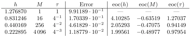
6.3. Moving surface. We consider the ellipsoid
Γ(t) =
x= (x1, x2, x3)∈R3
x
2 1 a(t)+x
2
2+x23= 1
with oscillatingx1-axisa(t) = 1 + 14sin(t), the velocity
v(t) =
x
1a(t)
2a′(t),0,0
T
,
andT = 1. The random diffusion coefficientαoccurring inah(·,·) is given by
α(x, ω) = 1 +x21+Y1(ω)x41+Y2(ω)x42,
whereY1 andY2denote independent, uniformly distributed random variables on Ω =
(−1,1). Observe thatAssumption 2.1and2.2are satisfied for this choice. The right-hand side f in (6.1) is chosen such that for each ω ∈ Ω the exact solution of the resulting path-wise problem is given by
u(x, t, ω) = sin(t)x1x2+Y1(ω) sin(2t)x21+Y2(ω) sin(2t)x2,
which clearly has a path-wise strong material derivative for all ω ∈Ω and satisfies the regularity property (5.19). As before, we select the initial condition u0(x, ω) = u(x,0, ω) = 0 so that (5.20) holds true.
The initial triangular approximation Γh,0 of Γ(0) is depicted in Figure 2for the
mesh sizesh=hj, j = 0, . . . ,3. We select the corresponding time step sizesτ0= 1,
Fig. 2.Triangular approximationΓh,0 ofΓ(0)forh=h0, . . . , h3.
τj = τj−1/4 and the corresponding numbers of samples M1 = 1, Mj = 16Mj−1 for j = 1,2,3. The resulting discretization errors (6.2) are shown in Table 5. Again, we observe that the discretization error behaves likeO(h2+M−1/2+τ). This is in
[image:26.612.92.420.508.571.2]accordance with our theoretical findings stated in Theorem 5.10 and fully discrete deterministic results [18, Theorem 2.4].
Table 5
Discretization errors for a moving surface inR3.
h M τ Error eoc(h) eoc(M) eoc(τ)
1.276870 1 1 9.91189·10−1 — — —
0.831246 16 4−1 1.70339·10−1 4.10285 −0.63519 1.27037
0.440169 256 4−2 4.61829·10−2 2.05293 −0.47075 0.94149
0.222895 4 096 4−3 1.18779·10−2 1.99561 −0.48977 0.97954