DOI 10.1007/s00285-016-1020-6
Mathematical Biology
Stochastic descriptors to study the fate and potential
of naive T cell clonotypes in the periphery
J. R. Artalejo1 · A. Gómez-Corral1,2 · M. López-García3 · C. Molina-París3
Received: 31 March 2015 / Revised: 20 April 2016 / Published online: 27 June 2016 © The Author(s) 2016. This article is published with open access at Springerlink.com
Abstract The population of naive T cells in the periphery is best described by deter-mining both its T cell receptor diversity, or number of clonotypes, and the sizes of its clonal subsets. In this paper, we make use of a previously introduced mathematical model of naive T cell homeostasis, to study the fate and potential of naive T cell clono-types in the periphery. This is achieved by the introduction of several new stochastic descriptors for a given naive T cell clonotype, such as its maximum clonal size, the time to reach this maximum, the number of proliferation events required to reach this maximum, the rate of contraction of the clonotype during its way to extinction, as well as the time to a given number of proliferation events. Our results show that two fates can be identified for the dynamics of the clonotype: extinction in the short-term if the clonotype experiences too hostile a peripheral environment, or establishment in the periphery in the long-term. In this second case the probability mass function for the maximum clonal size is bimodal, with one mode near one and the other mode far away from it. Our model also indicates that the fate of a recent thymic emigrant (RTE) during its journey in the periphery has a clear stochastic component, where the probability of extinction cannot be neglected, even in a friendly but competitive environment. On the other hand, a greater deterministic behaviour can be expected in the potential size of the clonotype seeded by the RTE in the long-term, once it escapes extinction.
B
C. Molina-París1 Department of Statistics and Operations Research, Faculty of Mathematics,
Complutense University of Madrid, 28040 Madrid, Spain
2 Instituto de Ciencias Matemáticas, CSIC-UAM-UC3M-UCM, Calle Nicolás Cabrera 13-15,
Campus de Cantoblanco UAM, 28049 Madrid, Spain
3 Department of Applied Mathematics, School of Mathematics, University of Leeds,
Keywords T cell homeostasis·TCR diversity·Stochastic univariate birth and death process·Extinction·Stochastic descriptor·Competition·Cross-reactivity
Mathematics Subject Classification 60J28 Applications of continuous-time Markov processes on discrete state spaces·92B05 General biology and biomathematics
1 Introduction
T cells are the set of lymphocytes characterised by the expression of a specialised receptor, called the T cell receptor (TCR). T cells can thus, be classified in “families” (or clonotypes) according to the molecular structure of the TCR they display on their membrane (Murphy et al. 2008). On average a T cell expresses 3×10⁴identical copies of a given TCR molecule. The number of T cells in the adaptive immune system of an adult human tends to a stationary “homeostatic” distribution (McLean et al. 1997;
Freitas and Rocha 2000), specified by its size (the total number of T cells) and TCR
diversity (the number of different clonotypes or TCR molecular structures). The size and diversity of the naive T cell pool (those T cells that have not taken part in a previous immune response) is essential to recognise a broad range of pathogens (Freitas and
Rocha 1999, 2000;Tanchot and Rocha 1998). An adult mouse has a homeostatic
population of 108naive T cells (Mason 1998) and a TCR diversity estimated around 2×
106(Zarnitsyna et al. 2013), and a healthy adult human has a homeostatic population
of 1011naive T cells (Hazenberg et al. 2003) distributed in 2.5×10⁷different TCR specificities (Zarnitsyna et al. 2013;Johnson et al. 2014).
Naive T cells originate from T cell precursors (or thymocytes) that survive positive and negative selection in the thymus (Stritesky et al. 2012;Moran and Hogquist 2012;
Bird 2009). Thus, naive T cells have not been activated by exposure to
pathogen-derived peptide fragments or antigens. During their lifetime, naive T cells constantly circulate in the blood to visit lymph nodes, which we refer to as the “periphery” (Takada
and Jameson 2009). The population of naive T cells, which have never taken part in an
immune response, is maintained by continuous, yet slow, division in the periphery (or homeostatic proliferation) (Tanchot and Rocha 1998;Troy and Shen 2003;Takada and
Jameson 2009). Antigen presenting cells provide the stimulatory signals that induce
1997) and stochastic (Stirk et al. 2008) models. Yet, the question of how the naive T cell population remains diverse is still not completely understood (De Boer et al.
2012).
During the homeostatic period the organisation of the peripheral naive T cell pool requires that an existing T cell must die if a new T cell is generated in the thymus or by peripheral cell division (Tanchot and Rocha 1998). It is then reasonable to pose a second challenge: to quantify the probability that a given TCR specificity, namely, a single recent thymic emigrant (RTE), can be established in the periphery, while competing with the pre-existing population of naive T cells. Recent thymic emigrants are those naive T cells that have just migrated out of the thymus, after surviving positive and negative selection, to become part of the peripheral T cell population (Fink 2013). Given that double positive thymocytes hardly divide in the thymic cortex and that single positive thymocytes divide at most once in the medulla of the thymus (Sinclair et al.
2013;Stritesky et al. 2013;Sawicka et al. 2014;Yates 2014), one expects a given TCR
specificity to be introduced in the periphery by a single recent thymic emigrant. There is evidence to support the fact that RTEs do not have an intrinsic lifespan (Tanchot
and Rocha 1998). Given the requirement of naive T cells for continuous TCR ligation
to survive in the periphery, it is natural to hypothesise that the TCR cross-reactivity of a given RTE (how many self-peptides can provide a homeostatic stimulus to the TCR under consideration) (Sewell 2012), the number of different clonotypes (competitor clonotypes) that can bind those self-peptides, and the clonal size of each competitor, are key parameters that will determine the fate and potential in the periphery of a recent thymic emigrant.
The aim of this paper is to make use of a previously introduced mathematical model of naive T cell homeostasis (Stirk et al. 2008,2010), and define new stochastic descriptors that allow us to provide answers to the previous questions. In Refs.Stirk
et al.(2008,2010), a continuous time birth and death Markov model that describes the
time evolution of a peripheral naive T cell clonotype was introduced. In this reference, it was shown that extinction takes place with certainty for all parameter values of the model, and the average time to extinction was computed. However, the question of how the affinity and the cross-reactivity of a given T cell clonotype (or RTE) determines (1) its ability to become part of the peripheral naive T cell repertoire, (2) its maximum size if the clone is to get established in the naive peripheral pool, and (3) the timescale to get established in the periphery at its maximum size, was not considered. We study these questions by defining novel stochastic descriptors for a given TCR clonotype or RTE.
2 Mathematical model
We make use of the mathematical model introduced inStirk et al.(2008) to describe the time evolution of the number of cells in a given T cell clonotype, that is, the number of naive T cells that express identical T cell receptor molecules. The main assumption of the model is that T cells of a given clonotype compete for signals delivered by molecules (self-peptides also referred to as pMHC) expressed on antigen presenting cells (APCs). These signals induce one round of cell division, that is, a birth event. All cells of the given clonotype can also die and this is a death event in the model.
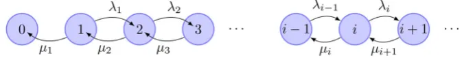
The underlying mathematical model is a birth and death process{X(t):t ≥0}on the state spaceX =N∪ {0}, where the random variableX(t)describes the number of cells of a given T cell clonotype as a function of timet. Its birth and death rates (Fig.1) are specified fori∈N∪ {0}byStirk et al.(2008):
λi =ϕ e−ν ∞
r=0
νr
r! i rn +i,
μi =μi. (1)
Parametersν ≥ 0,μ > 0, ϕ > 0, andn ≥ 1 were introduced in Stirk et al.
(2008), and they have the following meaning:
• μis the per (naive) cell death rate for cells of the clonotype under consideration,
• ϕis the per (naive) cell rate of homeostatic proliferation due to signals from the self-peptides that can bind to the TCR of the clonotype under consideration,
• νis the number of other clonotypes (different from the one under consideration) that can compete for the same homeostatic proliferation signals, and
• n is the characteristic size of T cell clonotypes that compete for homeostatic proliferation signals with the clonotype of interest. We note that these compet-ing clonotypes are not explicitly modelled and by assumcompet-ing that they all have a characteristic number of naive T cells given byn, the time evolution of the clono-type of interest can be reduced to a univariate Markov process (details about this approximation can be found in Stirk et al.(2008)).
It was shown in Stirk et al.(2008) that, for any value of the parameters, 0 ∈ X is an absorbing state of the stochastic process, the time to extinction (or absorption) from any other statei ∈Xis finite with probability one, and its mean is also finite.
As introduced above, parameterϕis a measure both of the affinity and the cross-reactivity of the T cell receptor for self-pMHC molecules (Sewell 2012), in the sense that the rate of homeostatic proliferation depends not only on how well a TCR can
[image:4.439.50.387.538.582.2]bind a given pMHC complex, but how many different pMHC complexes can provide survival signals to the T cell clonotype under consideration, characterised by its TCR molecule. Parameterν is the number of competitors of the clonotype under consid-eration (Stirk et al.(2008)). Three regimes can be identified in parameter space that describe different immunological scenarios: the first one is the limit of no inter-clonal competition (ν 1), the second is the limit of large inter-clonal competition (ν 1), and the third one is the intermediate regime of competition (ν≈1).
Hard niche clonotype In the special caseν 1, the population under study (the number of T cells that belong to a given TCR clonotype) does not compete with any other clonotypes, and thus the previous expressions for the birth and death rates simplify to (Stirk et al.(2008))
λi =ϕ, μi =μi.
Soft niche clonotype The opposite limit, ν 1, represents a highly competitive environment, where the population of T cells under study competes with a large num-ber of different clonotypes, and thus the expressions for the birth and death rates become (Stirk et al.(2008))
λi = ϕ
i
νn +i,
μi =μi.
Intermediate niche clonotypeIn the caseν ≈1, the TCR clonotype will be referred to as an intermediate niche clonotype, and its birth and death rates will be given by Eq. (1).
These three regimes, hard, soft and intermediate niche clonotypes, will be explored in Sect.3. Under these regimes, we introduce in this Section several stochastic descrip-tors which will allow us to study the dynamics of the clonotype under consideration. In particular, in Sect.2.1our interest is in the maximum clonal size reached by the clonotype and the time to reach this maximum size, for which we obtain analytical expressions for its probability mass function and its different order moments, respec-tively. We analyse the number of proliferation events to reach the maximum clonal size in Sect.2.2, and in Sect.2.3we focus on the time to reach a given number of pro-liferation (or division) events, as a measure of the proliferative capacity (or potential) of the clonotype under study. Finally, the rate of contraction of the clonotype during its way to extinction can be studied by means of the time to contraction to a given clonal size, which is also analysed in Sect.2.1.
2.1 Maximum clonal size and time to reach it
Xmaxi =max{X(t):t ≥0|X(0)=i}, Timax =inf{t :X(t)=Ximax},
fori ∈X, which amount to the maximum clonal size attained by the clonotype, under the assumption that the initial size equalsi, and the time to reach this maximum clonal size, respectively; note thatX0max =0 andT0max =0, since 0 is an absorbing state in
X. In order to study both variables in parallel, we define the time to reach a total clonal sizei, given that the initial clonal size equalsi, as the auxiliary random variable
Ti,i =inf{t :X(t)=i|X(0)=i},
fori,i∈X, withTi,i =0. We point out here that these auxiliary random variables
have their own immunological interest, since attaining a given clonal sizei might indicate that the clonotype has become large enough to mount an immune response in a timely fashion, or it has grown too large and might lead to autoimmunity, so that a tolerant immune state has been lost. The analysis ofTi,ialso allows the study of the
random variables of interestXimaxandTimax.
For a particular clonal sizei ∈ X, the random variableTi,i might be analysed
in a different manner depending on whetheri < i (time tocontractionto a given clonal sizei), ori>i(time toexpansionto a given clonal sizei). We note that in the latter case, reachingiis not certain, so thatTi,i is a defective random variable,
while reachingiis certain in the former case, since absorption at state 0 occurs with probability one (Stirk et al. 2008).
2.1.1 Time to contraction to a given clonal size i<i , given the initial clonal size i
For an initial clonal sizeiwithi >i, the random variableTi,iamounts to the time
until absorption intoi for a birth and death process defined on a single absorbing statei and the class of transient states,{i+1,i+2, . . .}, with birth rates{λj :
j ≥i+1}and death rates{μj : j ≥i+1}. Since absorption of the underlying
process{X(t):t ≥0}occurs in a finite time almost surely (see Stirk et al.(2008)), an appeal to Karlin and McGregor(1957) allows us to describe the expected values ofTi,i from the equality
E
Tik,i
=k
i−1
n=i
ρn ∞
j=n+1
E
Tjk,−i1
λj ρj ,
k≥1,
whereρi =1 andρn=
n
k=i+1λ−
1
k μk, forn≥i+1; note that the expected values
E[Tik,0]corresponding toi=0 are related to the total extinction of the clonotype. We refer the reader to Artalejo et al.(2012), where an analogous descriptor is analysed for the spread of an SIS epidemic among a population consisting ofNindividuals. In this case, the series∞j=n+1becomes the finite sumNj=n+1andTi,ican be seen as
a phase-type random variable (see e.g., [Kulkarni(1996), Sect. 6.7] and [Latouche
2.1.2 Time to expansion to a given clonal size i>i , given the initial clonal size i , and analysis of Ximax and Timax
For a fixed (and given) clonal sizei∈N, we introduce the following notation:
vi,i =P(Ti,i <∞) = P(Xmaxi ≥i), 0≤i ≤i, φi,i(s)= E
e−s Ti,i 1
{Ti,i<∞}
, 0≤i≤i, (s)≥0, (2)
m(i,ki)
= E
Ti,i
k
1{Ti,i<∞}
= (−1)k d
k
dskφi,i(s)
s=0
, 0≤i≤i, k≥0,
where 1{Ti,i<∞} is a random variable that takes the values 1 ifTi,i < ∞, and 0
otherwise. The quantities defined in Eq. (2) will allow us to analyse the random variablesXmaxi andTimax, but the distribution ofTi,i is defective, sinceTi,i = ∞
if the clonotype becomes extinct before reaching the sizei; note that 1−vi,iis the
probability of such an extinction event, as
vi,i =
0, ifi=0, 1, ifi=i,
withvi,i ∈(0,1)in the case 1≤i ≤i−1.
By a first-step argument, the restricted Laplace-Stieltjes transforms satisfy the fol-lowing set of linear equations:
φ0,i(s)=0, φi,i(s)= μ
i
s+λi+μi φi−1,i(
s)+ λi
s+λi +μi φi+1,i(
s), 1≤i≤i−1,
φi,i(s)=1. (3)
These equations can be rewritten in multiplicative form as
βi φi−1,i(s)+γi φi,i(s)+αi φi+1,i(s)=δi, 1≤i ≤i−1,
with
αi =
−λi, if 1≤i ≤i−2,
0, if i =i−1,
βi =
0, if i =1,
−μi, if 2≤i ≤i−1,
γi =s+λi +μi, 1≤i ≤i−1, δi =
0, if 1≤i ≤i−2,
Then, by using forward elimination, we may obtain
Gi φi,i(s)+αi φi+1,i(s)=Di, 1≤i ≤i−1,
with
Gi =
γ1, ifi =1,
γi −βGiαi−i−1
1 , if 2≤i ≤i−1, Di =
0, if 1≤i≤i−2,
λi−1, ifi=i−1.
In terms of the functionsgi(s)=Gi −(s+λi), we may rewriteφi,i(s)as
φi,i(s)=
Di−αi φi+1,i(s)
s+λi+gi(s) ,
sincegi(s)satisfies
gi(s)=μi
s+gi−1(s) s+λi−1+gi−1(s),
2≤i ≤i−1,
withg1(s)=μ1. This implies that
φi,i(s)=
i−1
k=i
λk
s+gk(s)+λk,
1≤i≤i−1, (4)
from which it follows that vi,i ∈ (0,1) for clonal sizes 1 ≤ i ≤ i −1, since vi,i =φi,i(0).
In evaluating therestrictedmomentsm(i,ki), we first derive the probabilitiesvi,i as
the valuesφi,i(0)from Eq. (4). In particular, it is seen thatv0,i =0 and we can write
vi,i =
⎛ ⎝
i−1
m=0
ζm
⎞ ⎠
−1
i−1
k=0
ζk, 1≤i ≤i,
whereζ0=1 andζi =
i
k=1λ−
1
k μk, for 1≤i ≤i−1. Then, we have
m(i0,i)
=vi,i, 0≤i ≤i,
Momentsm(ik,i), for clonal sizes 1≤i ≤i−1, are derived from Eq. (3). In fact, by taking derivatives in Eq. (3) we obtain
(λi +μi)mi(,ki) =μi m(i−k)1,i+λi m(i+k)1,i+k m(i,ki−1), 1≤i ≤i−1, k≥1.
(5)
In order to solve Eq. (5), for a fixed valuek ≥ 1, we introduce some notation as follows:
xi,i =m(i,ki),
ξi,i =k mi(k,i−1), 0≤i ≤i,
yi,i =xi+1,i−xi,i, 0≤i ≤i−1.
Equation (5) is then equivalent toλi yi,i+ξi,i =μi yi−1,i, for 1≤i ≤ i−1,
which implies that
yi,i =ζi y0,i−ζi bi,
wherebi =ij=1 ξj,i
λjζj. As a result, for 1≤i ≤i−1, we have
xi+1,i =x1,i i
j=0
ζj− i
j=1
ζj bj.
We also havexi,i=0 sincemi(k,)i =0, so that
x1,i =
i−1
j=1 ζj bj
i−1
j=0 ζj
,
xi,i =
i−1
j=i ζj
i−1
m=0ζm
j
k=m+1
ξk,i
λkζk
i−1
j=0 ζj
, 2≤i ≤i−1, (6)
xi,i =0.
Equation (6) is a recursive procedure that allows us to compute thekth order moments, m(i,ki)
, in terms of previously computed moments, m
(k−1)
i,i , since xi,i = m(
k)
i,i and
ξi,i =k m(ik,i−1). In the special casesk=0 and 1, it is readily seen that
lim
i→∞vi,i =
0, if 0≤i ≤i−1, 1, ifi =i,
and the asymptotic value limi→∞m(i,1i)is always finite, with limi→∞m(i,1i) =0 for
We finally focus on the random variablesXimaxandTimax. Note that the distribution of Xmaxi is readily derived from the valuesvi,i, sincevi,i =P(Ximax ≥i), and the
kth order moment,mmaxi ,(k), of the timeTimax to reach the maximum clonal size can be evaluated as
mmaxi ,(k)=
∞
i=i
ETimaxk Ximax =i
P(Ximax =i)
= ∞
i=i+1
m(i,ki)
1−vi,i+1
vi,i
.
For practical or computational purposes, the above series should be replaced by the finite sum
Kq
i=i+1
m(ik,i)
1−vi,i+1
vi,i
, (7)
where Kq can be selected as the (100q)th percentile of Xmaxi for a probability
q ∈ (0,1)close enough to 1. Although an analytical study ofi∞=Kq+1m(ik,i)(1−
v−1
i,ivi,i+1)does not seem to be feasible, we note that by using the finite sum in Eq. (7)
we ensure that the probability mass accumulated by Xmaxi is greater thanq, whence the probability 1−q can be interpreted as a global error measure. Furthermore, this type of truncation procedure has been efficiently used for epidemics (Almaraz et al. 2016) and competition processes (Gómez-Corral and López García 2011,2012).
2.2 Number of proliferation events to reach the maximum clonal size
We are now interested in the number Nimax of one-step transitionsi →i+1 ofX occurring in the random interval[0,Timax], which allows us to record the number of proliferation events to reach the maximum clonal size, fori ∈X. This descriptor can be seen as a discrete version of the random variableTimax in Sect. 2.1, and its analysis can be carried out by means of the number of proliferation events to reach a total clonal size, which is defined as the numberNi,iof one-step transitionsi→i+1 ofXto
registerX(t)=ifor the first time.
We first introduce the following notation:
ψi,i(z)=E
zNi,i 1
{Ni,i<∞}
, |z| ≤1, ui,i =P(Ni,i <∞),
˜
m(i,ki)
=E
Ni,i(Ni,i−1)· · ·(Ni,i−k+1)1{Ni,i<∞}
for initial clonal sizes 1 ≤ i ≤ i. It can be easily verified thatψ0,i(z)= u0,i = ˜
m(0k,i)
= 0,ψi,i(z)= ui,i =1 andm˜
(k)
i,i = 0, fork ≥ 1. For clonal sizes 1 ≤
i ≤i−1, it is seen thatui,i =vi,i, sinceψi,i(1)=φi,i(0)and, consequently, the
probabilitiesui,ican be computed from Eq. (4), and they amount to the probabilities
of reaching the clonal sizeibefore extinction, given that the initial clonal size isi. By taking derivatives on the equality
ψi,i(z)= μ i
λi +μi ψi−1,i(
z)+ λi
λi+μi
zψi+1,i(z), 1≤i ≤i−1,
we obtain
(λi+μi)m˜(ik,i) =μi m˜(ik−)1,i+λi m˜i(k+)1,i+λi km˜i(+k−11,i), 1≤i ≤i−1, k≥1,
(8)
which is similar to Eq. (5) with the termk m(ik,i−1) replaced byλi k m˜(ik+−11,i). This
implies that, similarly to the solution of Eq. (6), the solution of Eq. (8) has the form
˜
m(i,ki)
=
i−1
j=i ζj
i−1
m=0ζm
j
n=m+1
km˜(nk+−11,)i
ζn
i−1
j=0 ζj
, 1≤i ≤i−1, k≥1. (9)
Similarly to Sect. 2.1.2, it can be seen that limi→∞m˜(i,1i) is always finite, with
limi→∞m˜(i,1i)=0 for initial clonal sizesi ∈ {0,i}.
In the case of the random variableNi,i, not only everykth order factorial moment
can be obtained from Eq. (9), but also its distribution. We can write
˜
xij,i
=P(Ni,i = j), 0≤i≤i, j ≥i−i,
withx˜0j,i
=0 forj ≥0,x˜ j
i,i =1 ifj=0, and 0 ifj≥1,x˜ j
i,i=0 for 1≤i ≤i−1
and 0≤ j ≤i−i−1, andx˜i0,i
=0 for 0≤i≤i−1. For j≥1, we have
˜
x0j,i =0,
˜
xij,i
=
μi λi+μi ˜
xij−1,i
+
λi λi+μi ˜
xij+−11,i
, 1≤i ≤i−1,
˜
xij
,i =0,
so that a recursion on jandican be obtained in order to compute the probability mass function ofNi,i. The probability mass function obtained in this way is consistent with
Finally, the factorial moments of the random variableNimax can be approximated in a similar way as described for Eq. (7). In particular, if we denote m˜maxi ,(k) =
E[Nimax(Nimax−1)· · ·(Nimax−k+1)], we have
˜
mmaxi ,(k) =
∞
i=i+1
˜
m(i,ki)
1−vi,i+1
vi,i
≈
Kq
i=i+1
˜
m(i,ki)
1−vi,i+1
vi,i
. (10)
2.3 Time to reach a given number of proliferation events
In this section, we fix an initial clonal sizei and a number D ≥ 0 of proliferation events, and we study the timeTiD to reach a total number Dof proliferation events
(one-step transitionsi→i+1 ofX), withTi0 =0. In order to study this descriptor,
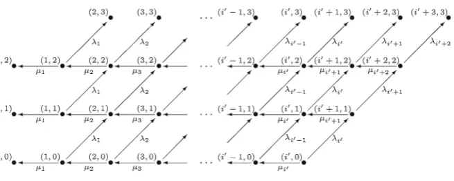
we consider the augmented process{(X(t),D(t)):t ≥0}, whereD(t)denotes the number of division events up to timet, with(X(0),D(0)) =(i,0). For the initial clonal sizei, the augmented process starts from state(i,0)and is defined on the finite state space
X0∪XD(i)∪XT(i),
where
X0= {(0,d):0≤d≤ D−1},
XD(i)= {(i,D):2≤i ≤i+D},
XT(i)= {(i,d):1≤i ≤i+d,0≤d ≤ D−1}.
States inX0∪XD(i)are absorbing states. In particular, states inX0represent the extinction of the clonotype when the number Dof proliferation events has not been reached, while states inXD(i)reflect that the number Dof proliferation events has
been reached. States inXT(i)are transient states. Figure2illustrates the dynamics
of the augmented process in the caseD=3.
In a more general setting, we define the random variable
T(Di,d) =inf{t :(X(t),D(t))∈XD(i)|(X(0),D(0))=(i,d)},
for states(i,d)∈X0∪XD(i)∪XT(i). Note that the descriptorTiD is equivalent to the
random variableT(Di,0), and states inX0andXD(i)lead to the valuesT
D
(0,d)= ∞and
T(Di,D) =0, respectively. For states inXT(i), the random variableT(Di,d)is defective,
Fig. 2 Transitions between augmented states in the caseD=3
For states(i,d)∈X0∪XD(i)∪XT(i), we introduce the notation
wD
(i,d)=P(T(Di,d)<∞), D
(i,d)(s)=E
e−sT(Di,d) 1
{TD
(i,d)<∞}
, (s)≥0,
ˆ
mD(i,,(dk))=E
T(Di,d)
k
1{TD (i,d)<∞}
, k≥0,
and we observe that
wD
(i,d)=
⎧ ⎨ ⎩
0, i f(i,d)∈X0,
∈(0,1), i f(i,d)∈XT(i),
1, i f(i,d)∈XD(i).
As a result, the Laplace-Stieltjes transformsD(i,d)(s)verify the boundary conditions
D
(0,d)(s) = 0 if (0,d) ∈ X0, and D
(i,D)(s) = 1 if (i,D) ∈ XD(i). For states (i,d)∈XT(i), we have
D
(i,d)(s)= μi
s+λi+μi D
(i−1,d)(s)+ λi
s+λi+μi D
(i+1,d+1)(s), (11)
which yields a finite system of linear equations that can be solved in a recursive manner (Algorithm 1).
The boundary conditions for the momentsmˆ(Di,,(dk))are given by
ˆ
m(Di,,(d0))=w(Di,d), (i,d)∈X0∪XD(i)∪XT(i), ˆ
[image:13.439.59.387.51.182.2]Algorithm 1 Computation of the Laplace-Stieltjes transforms (Di,d)(s) for states (i,d) ∈
X0∪XD(i)∪XT(i).
Step 1: d:=D;
i:=1;
whilei<i+d, do
i:=i+1;
D
(i,d)(s):=1;
enddo.
Step 2:Whiled>1, do
d:=d−1;
i:=0;
D
(i,d)(s):=0;
whilei<i+d, do
i:=i+1;
D
(i,d)(s):=
μiD(i−1,d)(s)+λiD(i+1,d+1)(s)
s+λi+μi ;
enddo; enddo.
where the probabilitiesw(Di,d), for states(i,d)∈XT(i), are derived from Algorithm 1
by selectings=0. If we take derivatives in Eq. (11), we may write down
ˆ
m(Di,,(dk)) = k
λi+μi ˆ
m(Di,,(dk)−1)+ μi
λi+μi ˆ
m(Di−,(k1),d)+ λi
λi +μi ˆ
m(Di+,(k1,)d+1), (12)
for states (i,d) ∈ XT(i). Eq. (12) can be solved (Algorithm 2) by adapting our arguments in Algorithm 1.
3 Numerical results
In this Section we carry out a set of numerical experiments in order to analyse the potential of a recent thymic emigrant (of a given clonotype) in the periphery to expand to different clonal sizes, or to proliferate for a given number of divisions, as well as the random times of these events, and the rate of contraction of the clonotype under consideration. We study these random variables under several competition and signalling environments, which are specified by the choice of parametersν,nand
ϕ. We point out here that parametersϕandνshould be seen as intrinsically related to the particular TCR expressed by the T cells within the clonotype under consideration, since this TCR determines the number of different self-peptides that the T cell can interact with. On the other hand, n is not directly related to the TCR and should be considered an environmental parameter, since it is the characteristic size of the competing clonotypes. We set the per cell death rateμ=1, so that the time unit in the process under study is the mean lifetime of a T cell.
Algorithm 2Computation of the momentsmˆ(Di,,(dk))for states(i,d)∈X0∪XD(i)∪XT(i).
Step 1: k:=0;
d:=D;
i:=1;
whilei<i+d, do
i:=i+1;
ˆ
m(Di,,(dk)):=1;
enddo; whiled>1, do
d:=d−1;
i:=0;
ˆ
m(Di,,(dk)):=0;
whilei<i+d, do
i:=i+1;
ˆ
m(Di,,(dk)):=μimˆ
D,(k)
(i−1,d)+λimˆD,(k ) (i+1,d+1)
λi+μi ;
enddo; enddo.
Step 2:Whilek<k, do
k:=k+1;
d:=D;
i:=1;
whilei<i+d, do
i:=i+1;
ˆ
m(Di,,(dk)):=0;
enddo; whiled>1, do
d:=d−1;
i:=0;
ˆ
m(Di,,(dk)):=0;
whilei<i+d, do
i:=i+1;
ˆ
m(Di,,(dk)):=kmˆ
D,(k−1) (i,d) +μimˆ
D,(k) (i−1,d)+λimˆ
D,(k) (i+1,d+1)
λi+μi ;
enddo; enddo; enddo;
niche cases amount to values of the signalling rateϕ, the numberνof competitors, and the characteristic sizenof these competitors ranging fromfriendlyscenarios, where the T cell clonotype under consideration can become established in the periphery, to hostileenvironments, where this establishment is not possible at all. In particular, we analyse:
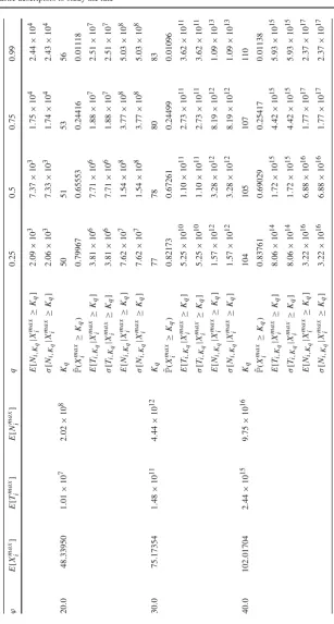
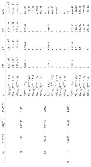
Ta b le 1 Expected v alues E [ X max i ] , E [ T max i ] and E [ N max i ] as a function o f ϕ for the hard niche case ( i.e ., ν = 0 ), for parameters μ = 1 . 0a n d i = 1 ϕ E [ X max i ] E [ T max i ] E [ N max i ] q 0 . 25 0 . 50 . 75 0 . 99 0 . 11 . 08143 0.07834 0 . 08617 Kq 11 1 2
˜P(X max i ≥ Kq ) 0 . 99526 0 . 99526 0 . 99526 0 . 08617 E [
Ti,
Kq | X max i ≥ Kq ] 00 0 0 . 90909 σ [
Ti,
Kq | X max i ≥ Kq ] 00 0 0 . 90909 E [
Ni,
Kq | X max i ≥ Kq ] 00 0 1 σ [
Ni,
Kq | X max i ≥ Kq ] 00 0 0 1 . 01 . 84694 0.52477 1 . 07984 Kq 12 3 5
˜P(X max i ≥ Kq ) 0 . 99351 0 . 49351 0 . 24351 0 . 02292 E [
Ti,
Kq | X max i ≥ Kq ] 00 . 51 . 25 2 . 79412 σ [
Ti,
Kq | X max i ≥ Kq ] 00 . 51 . 03078 2 . 03962 E [
Ni,
Kq | X max i ≥ Kq ] 01 2 . 56 . 29412 σ [
Ni,
Kq | X max i ≥ Kq ] 00 0 . 86603 2 . 66205 5 . 08 . 40494 12.72341 67 . 15374 Kq 41 01 21 6
˜P(X max i ≥ Kq ) 0 . 74812 0 . 54931 0 . 32916 0 . 00999 E [
Ti,
Kq | X max i ≥ Kq ] 0 . 72892 9 . 43564 21 . 56767 39 . 98014 σ [
Ti,
Kq | X max i ≥ Kq ] 0 . 52755 8 . 08455 19 . 77093 37 . 53902 E [
Ni,
Kq | X max i ≥ Kq ] 4 . 02410 49 . 43688 113 . 44516 214 . 03020 σ [
Ni,
Kq | X max i ≥ Kq ] 1 . 43975 39 . 26485 98 . 40159 191 . 6886 10 . 02 1 . 50413 927.95677 9 . 29 × 10 3 Kq 22 24 26 29
˜P(X max i ≥ Kq ) 0 . 80227 0 . 61532 0 . 25744 0 . 01306 E [
Ti,
Kq | X max i ≥ Kq ] 209 . 05940 736 . 272000 1745 . 83800 2435 . 43200 σ [
Ti,
Ta b le 1 continued ϕ E [ X max i ] E [ T max i ] E [ N max i ] q 0 . 25 0 . 50 . 75 0 . 99 E [
Ni,
Kq | X max i ≥ Kq ] 2 . 09 × 10 3 7 . 37 × 10 3 1 . 75 × 10 4 2 . 44 × 10 4 σ [
Ni,
Kq | X max i ≥ Kq ] 2 . 06 × 10 3 7 . 33 × 10 3 1 . 74 × 10 4 2 . 43 × 10 4 20 . 04 8 . 33950 1 . 01 × 10 7 2 . 02 × 10 8 Kq 50 51 53 56
˜P(X max i ≥ Kq ) 0 . 79967 0 . 65553 0 . 24416 0 . 01118 E [
Ti,
Kq | X max i ≥ Kq ] 3 . 81 × 10 6 7 . 71 × 10 6 1 . 88 × 10 7 2 . 51 × 10 7 σ [
Ti,
Kq | X max i ≥ Kq ] 3 . 81 × 10 6 7 . 71 × 10 6 1 . 88 × 10 7 2 . 51 × 10 7 E [
Ni,
Kq | X max i ≥ Kq ] 7 . 62 × 10 7 1 . 54 × 10 8 3 . 77 × 10 8 5 . 03 × 10 8 σ [
Ni,
Kq | X max i ≥ Kq ] 7 . 62 × 10 7 1 . 54 × 10 8 3 . 77 × 10 8 5 . 03 × 10 8 30 . 07 5 . 17354 1 . 48 × 10 11 4 . 44 × 10 12 Kq 77 78 80 83
˜P(X max i ≥ Kq ) 0 . 82173 0 . 67261 0 . 24499 0 . 01096 E [
Ti,
Kq | X max i ≥ Kq ] 5 . 25 × 10 10 1 . 10 × 10 11 2 . 73 × 10 11 3 . 62 × 10 11 σ [
Ti,
Kq | X max i ≥ Kq ] 5 . 25 × 10 10 1 . 10 × 10 11 2 . 73 × 10 11 3 . 62 × 10 11 E [
Ni,
Kq | X max i ≥ Kq ] 1 . 57 × 10 12 3 . 28 × 10 12 8 . 19 × 10 12 1 . 09 × 10 13 σ [
Ni,
Kq | X max i ≥ Kq ] 1 . 57 × 10 12 3 . 28 × 10 12 8 . 19 × 10 12 1 . 09 × 10 13 40 . 0 102 . 01704 2 . 44 × 10 15 9 . 75 × 10 16 Kq 104 105 107 110
˜P(X max i ≥ Kq ) 0 . 83761 0 . 69029 0 . 25417 0 . 01138 E [
Ti,
Kq | X max i ≥ Kq ] 8 . 06 × 10 14 1 . 72 × 10 15 4 . 42 × 10 15 5 . 93 × 10 15 σ [
Ti,
Kq | X max i ≥ Kq ] 8 . 06 × 10 14 1 . 72 × 10 15 4 . 42 × 10 15 5 . 93 × 10 15 E [
Ni,
Kq | X max i ≥ Kq ] 3 . 22 × 10 16 6 . 88 × 10 16 1 . 77 × 10 17 2 . 37 × 10 17 σ [
Ni,
[image:17.439.69.377.39.613.2]Ta b le 1 continued ϕ E [ X max i ] E [ T max i ] E [ N max i ] q 0 . 25 0 . 50 . 75 0 . 99 50 . 0 128 . 84185 4 . 28 × 10 19 2 . 14 × 10 21 Kq 131 132 134 1 37
˜P(X max i ≥ Kq ) 0 . 85166 0 . 70967 0 . 26879 0 . 01220 E [
Ti,
Kq | X max i ≥ Kq ] 1 . 30 × 10 19 2 . 84 × 10 19 7 . 60 × 10 19 1 . 04 × 10 20 σ [
Ti,
Kq | X max i ≥ Kq ] 1 . 30 × 10 19 2 . 84 × 10 19 7 . 60 × 10 19 1 . 04 × 10 20 E [
Ni,
Kq | X max i ≥ Kq ] 6 . 52 × 10 20 1 . 42 × 10 21 3 . 80 × 10 21 5 . 19 × 10 21 σ [
Ni,
Kq | X max i ≥ Kq ] 6 . 52 × 10 20 1 . 42 × 10 21 3 . 80 × 10 21 5 . 19 × 10 21 75 . 0 196 . 43319 2 . 06 × 10 30 1 . 55 × 10 32 Kq 199 200 201 2 05
˜P(X max i ≥ Kq ) 0 . 83576 0 . 67186 0 . 44024 0 . 00960 E [
Ti,
Kq | X max i ≥ Kq ] 7 . 42 × 10 29 1 . 58 × 10 30 2 . 77 × 10 30 4 . 97 × 10 30 σ [
Ti,
Kq | X max i ≥ Kq ] 7 . 42 × 10 29 1 . 58 × 10 30 2 . 77 × 10 30 4 . 97 × 10 30 E [
Ni,
Kq | X max i ≥ Kq ] 5 . 57 × 10 31 1 . 19 × 10 32 2 . 07 × 10 32 3 . 73 × 10 32 σ [
Ni,
Kq | X max i ≥ Kq ] 5 . 57 × 10 31 1 . 19 × 10 32 2 . 07 × 10 32 3 . 73 × 10 32 100 . 0 264 . 12728 1 . 01 × 10 41 1 . 11 × 10 43 Kq 267 268 269 2 73
˜P(X max i ≥ Kq ) 0 . 81774 0 . 63708 0 . 39927 0 . 00800 E [
Ti,
Kq | X max i ≥ Kq ] 4 . 59 × 10 40 9 . 55 × 10 40 1 . 61 × 10 41 2 . 68 × 10 41 σ [
Ti,
Kq | X max i ≥ Kq ] 4 . 59 × 10 40 9 . 55 × 10 40 1 . 61 × 10 41 2 . 68 × 10 41 E [
Ni,
Kq | X max i ≥ Kq ] 4 . 59 × 10 42 9 . 55 × 10 42 1 . 61 × 10 43 2 . 68 × 10 43 σ [
Ni,
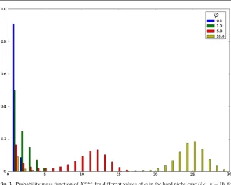
[image:18.439.83.362.34.615.2]Fig. 3 Probability mass function ofXimaxfor different values ofϕin the hard niche case (i.e.,ν=0), for μ=1.0 and the initial clonal sizei=1
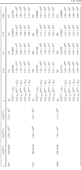
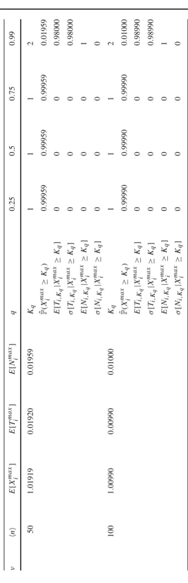
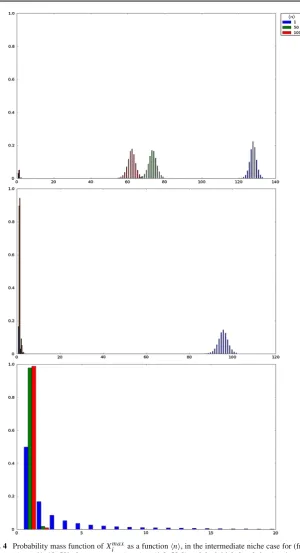
(b) The intermediate niche case in Table2and Fig.4, which corresponds to moder-ate average numbers of competitors,ν ∈ {1,10,50}, and moderate homeostatic signalling rates,ϕ =50,
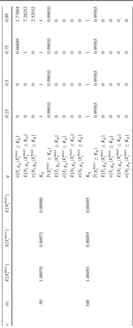
(c) The soft niche case in Table3and Fig.5, which reflects large average numbers of competitors,ν∈ {500,1000}, and high homeostatic signalling rates,ϕ=500. In Tables1,2and3, the mean valuesE[Ximax],E[Timax]andE[Nimax]are com-puted by considering only clonal sizes up to the 99th percentile K0.99 of Xmaxi , and
[image:19.439.53.384.46.311.2]Ta b le 2 Expected v alues E [ X max i ] , E [ T max i ] and E [ N max i ] for d if ferent choices of (ν , n ) in the intermediate niche case for the p arameters (μ ,ϕ ) = ( 1 . 0 , 50 . 0 ) and the initial clonal size i = 1 ν n E [ X max i ] E [ T max i ] E [ N max i ] q 0 . 25 0 . 50 . 75 0 . 99 1 1 123 . 25013 1 . 57 × 10 18 7 . 68 × 10 19 Kq 127 128 129 133
˜P(X max i ≥ Kq ) 0 . 78258 0 . 60668 0 . 38305 0 . 00847 E [
Ti,
Kq | X max i ≥ Kq ] 7 . 22 × 10 17 1 . 43 × 10 18 2 . 33 × 10 18 3 . 83 × 10 18 σ [
Ti,
Kq | X max i ≥ Kq ] 7 . 22 × 10 17 1 . 43 × 10 18 2 . 33 × 10 18 3 . 83 × 10 18 E [
Ni,
Kq | X max i ≥ Kq ] 3 . 54 × 10 19 7 . 00 × 10 19 1 . 14 × 10 20 1 . 88 × 10 20 σ [
Ni,
Kq | X max i ≥ Kq ] 3 . 54 × 10 19 7 . 00 × 10 19 1 . 14 × 10 20 1 . 88 × 10 20 50 68 . 61117 2 . 16 × 10 8 5 . 92 × 10 9 Kq 71 73 75 79
˜P(X max i ≥ Kq ) 0 . 83010 0 . 60581 0 . 27023 0 . 00942 E [
Ti,
Kq | X max i ≥ Kq ] 5 . 97 × 10 7 1 . 86 × 10 8 3 . 75 × 10 8 5 . 22 × 10 8 σ [
Ti,
Kq | X max i ≥ Kq ] 5 . 97 × 10 7 1 . 86 × 10 8 3 . 75 × 10 8 5 . 22 × 10 8 E [
Ni,
Kq | X max i ≥ Kq ] 1 . 64 × 10 9 5 . 10 × 10 9 1 . 03 × 10 10 1 . 43 × 10 10 σ [
Ni,
Kq | X max i ≥ Kq ] 1 . 64 × 10 9 5 . 10 × 10 9 1 . 03 × 10 10 1 . 43 × 10 10 100 57 . 61605 2 . 24 × 10 7 5 . 15 × 10 8 Kq 60 62 63 67
˜P(X max i ≥ Kq ) 0 . 78631 0 . 50329 0 . 32493 0 . 01130 E [
Ti,
Kq | X max i ≥ Kq ] 8 . 71 × 10 6 2 . 54 × 10 7 3 . 59 × 10 7 5 . 44 × 10 7 σ [
Ti,
Kq | X max i ≥ Kq ] 8 . 71 × 10 6 2 . 54 × 10 7 3 . 59 × 10 7 5 . 44 × 10 7 E [
Ni,
Kq | X max i ≥ Kq ] 2 . 01 × 10 8 5 . 85 × 10 8 8 . 27 × 10 8 1 . 25 × 10 9 σ [
Ni,
Kq | X max i ≥ Kq ] 2 . 01 × 10 8 5 . 85 × 10 8 8 . 27 × 10 8 1 . 25 × 10 9 10 1 7 5 . 87474 4 . 57 × 10 9 1 . 82 × 10 11 Kq 92 95 97 102
˜P(X max i ≥ Kq ) 0 . 75703 0 . 58015 0 . 30540 0 . 00584 E [
Ti,
Ta b le 2 continued ν n E [ X max i ] E [ T max i ] E [ N max i ] q 0 . 25 0 . 50 . 75 0 . 99 σ [
Ti,
Kq | X max i ≥ Kq ] 5 . 38 × 10 8 3 . 50 × 10 9 8 . 10 × 10 9 1 . 31 × 10 10 E [
Ni,
Kq | X max i ≥ Kq ] 2 . 15 × 10 10 1 . 40 × 10 11 3 . 23 × 10 11 5 . 24 × 10 11 σ [
Ni,
Kq | X max i ≥ Kq ] 2 . 15 × 10 10 1 . 40 × 10 11 3 . 23 × 10 11 5 . 24 × 10 11 50 1 . 11079 0 . 09735 0 . 11315 Kq 111 3
˜P(X max i ≥ Kq ) 0 . 99869 0 . 99869 0 . 99869 0 . 01028 E [
Ti,
Kq | X max i ≥ Kq ] 000 1 . 48326 σ [
Ti,
Kq | X max i ≥ Kq ] 000 1 . 14561 E [
Ni,
Kq | X max i ≥ Kq ] 000 2 . 10206 σ [
Ni,
Kq | X max i ≥ Kq ] 000 0 . 33538 100 1 . 04909 0 . 04937 0 . 05227 Kq 111 2
˜P(X max i ≥ Kq ) 0 . 99682 0 . 99682 0 . 99682 0 . 05227 E [
Ti,
Kq | X max i ≥ Kq ] 000 0 . 94455 σ [
Ti,
Kq | X max i ≥ Kq ] 000 0 . 94455 E [
Ni,
Kq | X max i ≥ Kq ] 000 1 σ [
Ni,
Kq | X max i ≥ Kq ] 000 0 50 1 2 . 99647 1 . 06499 4 . 53753 Kq 123 2 0
˜P(X max i ≥ Kq ) 0 . 99229 0 . 49229 0 . 32338 0 . 00242 E [
Ti,
Kq | X max i ≥ Kq ] 00 . 51 . 00676 10 . 60944 σ [
Ti,
Kq | X max i ≥ Kq ] 00 . 50 . 82202 6 . 66161 E [
Ni,
Kq | X max i ≥ Kq ] 012 . 33784 77 . 95166 σ [
Ni,
[image:21.439.68.377.49.617.2]Ta
b
le
2
continued
ν
n
E
[
X
max i
]
E
[
T
max i
]
E
[
N
max i
]
q
0
.
25
0
.
50
.
75
0
.
99
50
1
.
01919
0
.
01920
0
.
01959
Kq
1112
˜P(X max i
≥
Kq
)
0
.
99959
0
.
99959
0
.
99959
0
.
01959
E
[
Ti,
Kq
|
X
max i
≥
Kq
]
0000
.
98000
σ
[
Ti,
Kq
|
X
max i
≥
Kq
]
0000
.
98000
E
[
Ni,
Kq
|
X
max i
≥
Kq
]
0001
σ
[
Ni,
Kq
|
X
max i
≥
Kq
]
0000
100
1
.
00990
0
.
00990
0
.
01000
Kq
1112
˜P(X max i
≥
Kq
)
0
.
99990
0
.
99990
0
.
99990
0
.
01000
E
[
Ti,
Kq
|
X
max i
≥
Kq
]
0000
.
98990
σ
[
Ti,
Kq
|
X
max i
≥
Kq
]
0000
.
98990
E
[
Ni,
Kq
|
X
max i
≥
Kq
]
0001
σ
[
Ni,
Kq
|
X
max i
≥
Kq
]
[image:22.439.66.253.37.616.2]Fig. 4 Probability mass function ofXmaxi as a functionn, in the intermediate niche case for (fromtop
[image:23.439.63.364.45.599.2]Ta b le 3 Expected v alues E [ X max i ] , E [ T max i ] and E [ N max i ] for d if ferent choices of (ν , n ) in the soft n iche case, for the parameters (μ ,ϕ ) = ( 1 . 0 , 500 . 0 ) and the initial clonal size i = 1 ν n E [ X max i ] E [ T max i ] E [ N max i ] q 0 . 25 0 . 50 . 75 0 . 99 500 1 3 . 64779 1 . 36144 9 . 36164 Kq 1134 4
˜P(X max i ≥ Kq ) 0 . 99048 0 . 99048 0 . 32293 0 . 00066 E [
Ti,
Kq | X max i ≥ Kq ] 001 . 00166 23 . 19127 σ [
Ti,
Kq | X max i ≥ Kq ] 000 . 81786 14 . 13329 E [
Ni,
Kq | X max i ≥ Kq ] 002 . 33378 3 63 . 97348 σ [
Ni,
Kq | X max i ≥ Kq ] 000 . 66722 222 . 16995 50 1 . 01882 0 . 01884 0 . 01922 Kq 1112
˜P(X max i ≥ Kq ) 0 . 99961 0 . 99961 0 . 99961 0 . 01922 E [
Ti,
Kq | X max i ≥ Kq ] 0000 . 98039 σ [
Ti,
Kq | X max i ≥ Kq ] 0000 . 98039 E [
Ni,
Kq | X max i ≥ Kq ] 0001 σ [
Ni,
Kq | X max i ≥ Kq ] 0000 100 1 . 00970 0 . 00971 0 . 00980 Kq 1111
˜P(X max i ≥ Kq ) 0 . 99010 0 . 99010 0 . 99010 0 . 99010 E [
Ti,
Kq | X max i ≥ Kq ] 0000 σ [
Ti,
Kq | X max i ≥ Kq ] 0000 E [
Ni,
Kq | X max i ≥ Kq ] 0000 σ [
Ni,
Kq | X max i ≥ Kq ] 0000 1000 1 1 . 54331 0 . 34871 0 . 64267 Kq 1126
˜P(X max i ≥ Kq ) 0 . 99225 0 . 99225 0 . 32536 0 . 00795 E [
Ti,
Ta b le 3 continued ν n E [ X max i ] E [ T max i ] E [ N max i ] q 0 . 25 0 . 50 . 75 0 . 99 σ [
Ti,
Kq | X max i ≥ Kq ] 000 . 66689 1 . 77604 E [
Ni,
Kq | X max i ≥ Kq ] 0017 . 28252 σ [
Ni,
Kq | X max i ≥ Kq ] 0002 . 52032 50 1 . 00970 0 . 00971 0 . 00980 Kq 1111
˜P(X max i ≥ Kq ) 0 . 99010 0 . 99010 0 . 99010 0 . 99010 E [
Ti,
Kq | X max i ≥ Kq ] 0000 σ [
Ti,
Kq | X max i ≥ Kq ] 0000 E [
Ni,
Kq | X max i ≥ Kq ] 0000 σ [
Ni,
Kq | X max i ≥ Kq ] 0000 100 1 . 00493 0 . 00493 0 . 00495 Kq 1111
˜P(X max i ≥ Kq ) 0 . 99503 0 . 99503 0 . 99503 0 . 99503 E [
Ti,
Kq | X max i ≥ Kq ] 0000 σ [
Ti,
Kq | X max i ≥ Kq ] 0000 E [
Ni,
Kq | X max i ≥ Kq ] 0000 σ [
Ni,
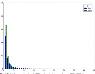
[image:25.439.61.289.45.607.2]Fig. 5 Probability mass function ofXimax in the soft niche case, forν ∈ {500,1000}, the parameters (μ, ϕ)=(1.0,500.0),n =1 and the initial clonal sizei=1
The distribution ofXimaxis analysed in Tables1,2and3by computing its(100q)th percentiles Kq for q ∈ {0.25,0.5,0.75,0.99}, where the percentile Kq is the first
value x ≥ 1, such that P(Ximax ≤ x) ≥ q. The probability P(Xmaxi ≥ Kq) of
reaching the clonal sizes represented by Kq can be exactly obtained from Eq. (4).
However, these probabilities are replaced in Tables 1,2 and3 by their truncated versionsP˜(Ximax ≥ Kq) = P(K0.99 ≥ Ximax ≥ Kq). We have done so as these
truncated values result in good approximations to the true probabilities, but with the advantage that, for the particular cases yieldingKq=1 (for example,ϕ ∈ {0.1,1.0}
andq =0.25 in Table1), they provide the total probability mass ofXimaxconsidered in the truncations given by Eqs. (7) and (10).
The time and the number of proliferation events to reach the maximum clonal size can be analysed in greater depth by studying the conditional valuesE[Ti,Kq|Ximax ≥
Kq],σ[Ti,Kq|Ximax ≥ Kq],E[Ni,Kq|Xmaxi ≥ Kq]andσ[Ni,Kq|Xmaxi ≥ Kq], where σ[X]denotes the standard deviation of the random variableX. We note here that we consider conditional values due to the fact that the random variablesTi,Kq andNi,Kq
are defective; that is, we haveTi,Kq =Ni,Kq = ∞if the clonal sizeKqis not reached,
which occurs with non-zero probability. These values provide information about the time and the number of proliferation events to reach different clonal sizes (Kq with
q ∈ {0.25,0.5,0.75,0.99}), under the assumption that those clonal sizes have been, in fact, reached.
[image:26.439.51.385.49.310.2]E[Timax]significantly larger than 1, which correspond to larger values of the homeosta-tic signalling rateϕ. It is clear that the mean value,E[Ximax], has a clearly increasing behaviour with respect to the signalling rateϕ. Moreover, results corresponding to those hostile environments within the hard niche case, corresponding to low signal rates, represent the pressure against the survival and expansion of the clonotype in the short-term. In those cases (ϕ ∈ {0.1,1.0,5.0}), the most representative sample path is the one which amounts to the immediate extinction of the clonotype from the initial clonal sizei = 1, which gives Ximax =1, or the occurrence of a few proliferation events (yielding a maximum size of the clonotype near 1), and the subsequent extinc-tion of the clonotype. On the other hand, in those cases where the clonotype survives in the mid-term (higher signalling rates), we observe a high concentration of the probabil-ity mass function of Xmaxi around some mode, which is reflected in the concentrated values obtained for the percentiles K0.25, K0.5, K0.75 and K0.99. In particular, the probability mass function of Xmaxi is unimodal when the clonotype becomes extinct in the short-term with high probability, and bimodal when the clonotype survives and expands in the mid-term, with moderate probabilities.
The bimodal shape of Xmaxi in friendly, yet competitive peripheral environments, within the hard niche case, becomes more apparent when analysing results plotted in Fig.3. In particular, we plot in Fig.3the probability mass function of Ximax for the hard niche case for signalling ratesϕ∈ {0.1,1.0,5.0,10.0}. The clonotype under consideration has higher potential for expansion for larger values of the homeostatic signalling rate ϕ. However, in these cases, the probability mass function of Xmaxi shows a bimodal shape, with a mode equal to 1 and the other taking different values depending on the particular parameters. This shape, together with the results of Table1, should be interpreted as a binary outcome scenario: in these cases, the clonotype has moderate or high probabilities of reaching its potential clonal size represented by the second mode, which will only happen if it escapes the extinction at the beginning of its lifetime; on the other hand, there exists, with some significant probability, the chance of the clonotype becoming extinct in the short-term (during its first transitions), which yields the first mode equal to 1. We point out here that this also means that (for example, see the caseϕ =10.0 in Fig.3), once the clonotype escapes extinction in the short-term, the probabilities of reaching different clonal sizes, such asi∈ {5,10,15}, are practically equal, since they represent the probability of reaching clonal sizes around the second mode. Finally, when the rate of signal is not enough (see the caseϕ=0.1 in Fig.3), the probability mass function ofXmaxi is unimodal around 1. This represents the case in which the clonotype will become immediately extinct (or extinct in the short-term after reaching small sizes around 1) from its initial clonal size 1.
The increase of E[Ximax] associated with increasing values of the homeostatic signalling rate in Table1leads also to increasing mean values forE[Timax],E[Nimax], E[Ti,Kq|Ximax ≥ Kq]andE[Ni,Kq|Xmaxi ≥ Kq]. This is easily explained by noting
that, in these cases, the clonotype has a greater potential to reach bigger clonal sizes, so that the time and number of proliferation events to reach those sizes should also be larger. The variability of these random variables increases, as well, which is observed by analysing the valuesσ[Ti,Kq|X
max
i ≥ Kq]andσ[Ni,Kq|X
max
i ≥ Kq]. Moreover,