Linear system identification of longitudinal vehicle dynamics versus nonlinear physical modelling

This is a repository copy of

Linear system identification of longitudinal vehicle dynamics

versus nonlinear physical modelling

.

White Rose Research Online URL for this paper:

http://eprints.whiterose.ac.uk/133010/

Version: Accepted Version

Proceedings Paper:

James, S. and Anderson, S.R. orcid.org/0000-0002-7452-5681 (2018) Linear system

identification of longitudinal vehicle dynamics versus nonlinear physical modelling. In:

Proceedings of 2018 UKACC 12th International Conference on Control (CONTROL).

Control 2018: The 12th International UKACC Conference on Control, 05-07 Sep 2018,

Sheffield, UK. IEEE , pp. 146-151. ISBN 978-1-5386-2864-5

https://doi.org/10.1109/CONTROL.2018.8516756

© 2018 IEEE. Personal use of this material is permitted. Permission from IEEE must be

obtained for all other users, including reprinting/ republishing this material for advertising or

promotional purposes, creating new collective works for resale or redistribution to servers

or lists, or reuse of any copyrighted components of this work in other works. Reproduced

in accordance with the publisher's self-archiving policy.

[email protected] https://eprints.whiterose.ac.uk/

Reuse

Items deposited in White Rose Research Online are protected by copyright, with all rights reserved unless indicated otherwise. They may be downloaded and/or printed for private study, or other acts as permitted by national copyright laws. The publisher or other rights holders may allow further reproduction and re-use of the full text version. This is indicated by the licence information on the White Rose Research Online record for the item.

Takedown

If you consider content in White Rose Research Online to be in breach of UK law, please notify us by

Linear System Identification of Longitudinal Vehicle

Dynamics Versus Nonlinear Physical Modelling

Sebastian James

and Systems Engineering University of Sheffield Sheffield, UK, S1 3JD Email: [email protected]

Sean R. Anderson

and Systems Engineering University of Sheffield Sheffield, UK, S1 3JD Email: [email protected]

Abstract—Mathematical modelling of vehicle dynamics is es-sential for the development of autonomous cars. Many of the vehicle models that are used for control design in cars are based on nonlinear physical models. However, it is not clear, especially for the case of longitudinal dynamics, whether such nonlinear models are necessary or simpler models can be used. In this paper, we identify a linear data-driven model of longitudinal vehicle dynamics and compare it to a nonlinear physically derived model. The linear model was identified in continuous-time state-space form using a prediction error method. The identification data were obtained from a Lancia Delta car, over 53 km of normal driving on public roads. The selected linear model was first order with requested torque, brake and road gradient as inputs and car velocity as output. The key results were that 1. the linear model was accurate, with a variance accounted for (VAF) metric of VAF=96.5%, and 2. the identified linear model was also superior in accuracy to the nonlinear physical model, VAF=77.4%. The implication of these results, therefore, is that for longitudinal dynamics, in normal driving conditions, a first order linear model is sufficient to describe the vehicle dynamics. This is advantageous for control design, state estimation and real-time implementation, e.g. in predictive control.

I. INTRODUCTION

Mathematical models of car vehicle dynamics are essen-tial for the development of future driverless cars and driver assistance systems [1]–[4]. Typically, the development of longitudinal and lateral vehicle control algorithms have been based on physically derived models, either fully nonlinear [5] or based on linearised time-varying models [6], [7]. These non-linear models lead to relatively complicated control and state estimation schemes, which are both challenging to implement in real-time and also challenging to analyse for stability.

Given that firstly, linear feedback control schemes are rela-tively tolerant of plant model error (e.g. due to nonlinearities), and secondly, nonlinearities in vehicles are relatively weak (although become important at high-g [8]), it would appear attractive to develop linear models of vehicle dynamics for control design. There are examples of linear models of vehicle dynamics identified from sampled data [9]. However, the relative utility of linear vehicle models have not yet been well investigated and compared to nonlinear physically-derived models.

The novel aim of this paper is to develop a linear model of longitudinal vehicle dynamics, compare it to a nonlinear

physically derived model and assess to what extent nonlinear modelling is necessary for vehicle control in normal driving.

To identify the model of longitudinal vehicle dynamics, we used experimental data combined with linear system identi-fication techniques. The experimental data were collected in a Lancia Delta car which was driven along a 53 km route on public roads in normal conditions. We used a prediction error method (PEM) to directly identify the linear model in continuous-time state-space form [10], with model initialisa-tion using subspace state-space system identificainitialisa-tion (N4SID) [11]. We used a constrained nonlinear optimisation routine to estimate parameters for a nonlinear physical model based on the longitudinal component of the well-known bicycle model of vehicle dynamics [12].

The results indicated that the linear model was comparable in accuracy to the nonlinear physical model and yet much simpler and more attractive for control design.

II. METHODS

A. Experimental data

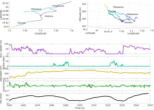
The experimental data used in modelling and identification were collected in a Lancia Delta car which was driven along a 53 km route on public roads in normal conditions. The route was chosen to incorporate a typical selection of motorways, extra-urban and urban roads, roundabouts and intersections. The route began at Centro Ricerche Fiat in Orbassano, near Turin (Italy), then went to Pinerolo via Piossasco before returning to Orbassano, a distance of 53 km driven in about 42 minutes, and is the same data as described in [3].

The following signals were amongst those recorded during the journey: longitudinal velocity, accelerator pedal position, brake pedal position, selected gear, engine torque and GPS co-ordinates. From the GPS co-ordinates, the road elevations were obtained (using the Google Maps API), providing the approximate road gradient. Signals were sampled at 20 Hz for the purpose of this modelling study. The elevation and road gradient signals were smoothed with a third order Butterworth low-pass filter with a cut-off frequency of 0.5 Hz.

Fig. 1. Test route of the Lancia Delta vehicle from the experiment conducted near Turin, Italy over 53 km of public roads in normal driving conditions, and example data over 100 seconds. The plot of road gradient shows the raw data and the smoothed data obtained from a zero-phase low-pass 3rd order Butterworth filter.

this into two sections; one of 2000 s duration for model identification and another of 1000 s for validation. Fig. 1 shows the control and output for part of the training data as an example.

B. Physical model of longitudinal vehicle dynamics

We employ a well known simplification of the physical dynamics of a four wheeled vehicle—that the lateral dynamics and the longitudinal dynamics may be decoupled [12]. The longitudinal model may then be expressed by its force equa-tion,

Mv˙=Fp(t) +Fb(t)−M gsin(γ(t))−kDv2−M g kR (1)

where M is the mass of the vehicle and v is the vehicle’s longitudinal velocity, which we will solve for. Fp(t) is the collective propulsive force due to the engine actuating through all of the drive wheels.Fb(t) is the collective braking force.

g is the acceleration due to gravity and γ(t) is the gradient of the road.kD is the parameter governing the strength of air resistance;kRis the static friction parameter. If operating with

velocity near 0 m/s, care must be taken to ensure that these frictional terms always act in the opposite direction tov.

While it is possible to model (for each gear) the relationship between the position of the accelerator pedal and Fp, the engine control unit (ECU) provides engine torque signals which can be used to compute the motive force. The ECU provides a requested engine torque signal, Ta, which is a scaled (0 to 400 Nm) version of the accelerator pedal position. When the requested engine torque is scaled by the gearbox ratio,R, we have a post-gearbox requested torque,Tr=Ta.R. The ECU also provides the delivered engine torque,Td, which may be lower than the requested torque if the engine is unable to comply with the request or if the engine torque is being controlled by the automatic gearbox during a gear shift. Additionally, the ECU reports the engine-speed dependent torque due to friction in the engine,Tf. The delivered engine-shaft torque, Te, is therefore given by

Te=Td−Tf (2)

Ta, and its post-gearbox partner, Tr, is most relevant, as the control system may not have access to the engine-friction signal or the ability to predict when the engine is unable to deliver the requested torque. However, the most accurate physical model against which to compare alternative models will be given by making use of the engine-shaft torque,

Te, along with the gear ratio information. In our physical modelling, we therefore haveFp given by

Fp(t) =

Te(t)R[G(t)]ηgRdηd

rw

(3)

where Te(t) is the delivered engine-shaft torque, R[G(t)] is the gearbox ratio as a function of the gear, G(t), and Rd is the driveline gear ratio. ηg and ηd model the frictional loss in the gearbox and driveline, respectively andrwis the wheel radius.R[G(t)]is provided by the ECU as a signal, which we combine withTe to give the pre-loss gear-shaft torque,Tg:

Tg(t) =Te(t)R[G(t)] (4)

We collect the terms Rd (unknown), ηd and ηg (unknown; approximately 0.93) andrw(known; 0.292 m) together into a single parameter,kτ, so thatFp is, finally,

Fp(t) =kτTg(t) (5)

with the value ofkτ to be found by the parameter search. The collective braking force, Fb(t), is governed by the relationship,

Fb(t) =   

 

µbM g v >0, kbpb(t)> µbM g

kbpb(t) v >0 0 otherwise

(6)

wherekb is a known coefficient of braking force in Newtons per bar of brake pressure (189 N/bar) andpb(t) is the time-varying master brake cylinder pressure. The upper limit on the available braking force,µbM g, is the force at which the tyres slip along the road surface; the coefficientµb is road-surface dependent. Because the data we use here were collected for normal driving, with no sharp or emergency braking taking place, we setµb to a high, fixed value for all time.

To estimate the parameters we used the training data and a nonlinear interior-point optimisation method [13], imple-mented in the MATLAB function fmincon. The parameters were initialised using a multi-start approach, with 100 different parameter sets, randomly sampled in the rangeskD∈[0,20],

kR∈[0,0.05]andkτ ∈[1,100]. We found the choice of ODE solver to be important in this work. MATLAB’sode23solver [14] operated well for the ‘best’ parameters—those which would provide a good fit to the data. However, this solver became computationally inefficient towards the boundaries of the chosen parameter ranges. For this reason, to allow the parameter search to complete quickly, theode23s solver [14] was employed, which is more effective in computing stiff differential equation systems. Unfortunately,ode23sproduced occasional, random, quickly corrected deviations from the putative true solution of the system, introducing noise into the

simulation and hence affecting the fit metrics. For this reason, after finding a first set of parameter values, we reduced the parameter ranges to kD ∈ [0.1,3], kR ∈ [0.0001,0.04] and

kτ ∈[5,15] and re-ran the parameter search usingode23and 30 different parameter sets as a start point. ode23was used when computing all simulations shown below and to generate the reported fit metrics.

C. Linear state-space system identification

For system identification, we used a linear continuous-time state-space model to represent the longitudinal vehicle dynamics:

˙

x(t) =Ax(t) +Bu(t) (7)

y(t) =Cx(t) +Du(t) (8)

where the output y(t) ∈ R is the vehicle velocity at time

t; the input u(t) ∈ Rnu

is composed of the delivered post-gearbox engine torque (Td) and the brake pressure signal (pb), and in some versions of the model also the smoothed road gradient (γ(t)); x(t)∈Rnx

is the vehicle state vector, where

nx is the model order, which is determined as part of the identification procedure. The matrices A, B, C and D are assumed fully parameterised here and comprise the unknown model parameters.

The parameters of the state-space model were estimated directly in continuous-time using a prediction error method (PEM) [10]. Assume all parameters in A, B, C and D are collected in the parameter vector θ_{, so that the estimation} problem is defined as

ˆ

θ_{= arg min} θ 1 N N X k=1

e(tk,θ)2 (9)

where the prediction error is e(tk,θ) =y(tk)−yˆ(tk,θ)and ˆ

y(tk,θ) is the simulated output of the state-space model at sample-timetk (N is the number of data samples). The PEM is typically solved using numerical search [10].

The numerical search algorithm can be initialised, as here, using a subspace state-space system identification (N4SID) algorithm [11]. The N4SID algorithm requires a number of choices (insight into these choices is given in [15]), such as the forward prediction horizon and the number of past inputs and outputs that are used for the prediction - here these were chosen by estimating multiple models over a range of values and using Akaike’s information criterion (AIC) to select between them. The weighting scheme used in the N4SID algorithm was canonical variate analysis (CVA) [16].

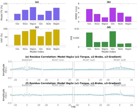
Fig. 2. Model selection for the linear system identification model, where the model index is as follows: t1o - torque only, first order; tb1o - torque-brake input, first order; tbg1o - brake-gradient input, first order; t2o - torque only, second order; tb2o - brake input, second order; tbg2o - torque-brake-gradient input, second order; (a)-(d) Model selection plots, which indicate that the models with torque-torque-brake-gradient inputs should be preferred. Note that FPE can be misleading because it is based on one-step-ahead prediction errors, unlike the other measures. (e)-(f) Residual analysis plots, which indicate that the first and second order models have similar auto-correlation in the model residuals and in the gradient input-residual cross-correlation.

that the N4SID identification was performed in discrete-time, then the model was mapped to continuous-time using a zero-order hold.

To select the model order,nx, model ordersnx= 1, . . . ,10 were initially tested using an analysis of singular values of the input-output covariance matrix [10], which suggested only models of first or second order should be further investi-gated. First and second order models were then analysed and compared with more in-depth methods, including Model Fit, Variance Accounted For (VAF), and residual analysis (see section below on model evaluation and validation).

To identify the model, the training data was used (com-prising 2000 seconds of normal driving data), which was consistent with the parameter estimation for the nonlinear physical modelling. A separate validation data set was used to validate the model (comprising a further 1000 seconds of normal driving data).

TABLE I

STATE-SPACESYSTEMIDENTIFICATIONALGORITHMPARAMETERS

Algorithm Option Method

Parameter Initialisation N4SID Initial State Estimated N4SID Weighting Scheme CVA N4SID Prediction Horizon Chosen by AIC

Loss Function Simulation Error Loss Function Weighting None

Search Method GN/AGN/LM/GD

D. Model evaluation and validation methods

Models were evaluated using a normalised fit metric based on the Euclidean norm of the fit error, where

Model Fit= 100

1−||y−yˆ||2 ||y−y¯||₂

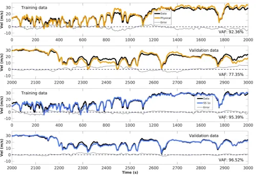
Fig. 3. Model simulations vs training and validation data. Top two rows: nonlinear physical model (orange) vs observed data (black). Bottom two rows: linear first order state-space model (blue) vs observed data (black). The residual error is shown in grey in each plot.

whereyis the vector of measured output data,yˆ is the vector of model simulation outputs, and ¯yis the mean of measured output data. A value of 100% indicates a perfect model fit, a value of 0% indicates a fit equivalent to the mean of the output data, and becomes negative for poor fits.

The model fit was also assessed using the variance ac-counted for (VAF) metric, which is equivalent to ther2_metric,

defined as

VAF= 100

1−var(y−yˆ)

var(y)

(11)

To evaluate the models in terms of accuracy and complexity, Akaike’s final prediction error (FPE) was used,

FPE= 1

N

N X

k=1

e₁(tk,θˆ)2× _{1 +n}

p/N 1−np/N

(12)

wherenpis the number of model parameters ande₁(.)denotes the one-step-ahead prediction error.

Residual analysis was also used in model validation, by analysing the auto-correlation of the residual error and the cross-correlation of the input and residual error [10].

III. RESULTS ANDDISCUSSION

The identification of the linear model first required the selection of model order. This was done with N4SID for orders

nx = 1, . . . ,10, using the singular values of the input-output covariance matrix, which indicated that a first, second or third order model should be chosen (results not shown). The first, second and third order models were then evaluated with three combinations of input: only, brake and torque-brake-gradient. The model evaluation methods indicated that inputs should consist of torque-brake-gradient as these models had the best fits to the data [Fig. 2(a)–(d))].

or the residual analysis, the first order model is preferred for its simplicity.

The linear first order model with torque-brake-gradient inputs (u1, u2, u3) was identified as

A=

−0.0008036

(13)

B=

0.0000016 −0.0000334 −0.0027613 (14)

C=

3499.522

(15)

D=

0 0 0

(16)

and the linear second order model with torque-brake-gradient inputs (u1, u2, u3) was identified as

A=

−0.2916319 0.0875774

−0.7851958 0.2345142

(17)

B=

−0.0000108 0.0003421 0.0042201

−0.0000325 0.0009946 0.0167971

(18)

C=

3313.131 −1278.718

(19)

D=

0 0 0

(20)

The nonlinear physical model parameters were estimated as

kD= 0.215,kR= 0.0214andkτ = 12.41.

Simulation comparison of the nonlinear physical model and linear first order model to each other and the observed data demonstrated that firstly both models were accurate predictors of car velocity, and that secondly the linear model was superior in accuracy to the nonlinear model (Fig. 3).

The overall VAF for the linear first order model was 96.5% and for the nonlinear physical model was 77.4%. There-fore, the linear state-space identified model outperformed the nonlinear model. More importantly, the accurate performance of the linear model is combined with the additional benefit of model simplicity, advantageous in tasks such as control and state-estimation.

There are few modelling studies that identify car vehicle dynamics from sampled data but one investigation that uses step responses found that a linear second order model was sufficient to accurately describe the car dynamics during single maneouvers of about 10 seconds duration [9]. That modelling study therefore agrees with the investigation here that linear models can be sufficient to describe vehicle dynamics.

A limitation of this investigation is that it only focuses on longitudinal vehicle dynamics. The lateral dynamics might require nonlinear modelling to adequately describe the car behaviour for full path control. In future work, therefore, we plan to extend the comparison of physical and linear identified models to the coupled longitudinal-lateral vehicle dynamics.

IV. CONCLUSION

In this paper, we have compared a nonlinear physical model of longitudinal car vehicle dynamics against a linear model obtained by system identification techniques. Experimental data used in the study was drawn from normal driving over 53 km of roads. A first order linear model, with torque-brake-gradient inputs, was found to accurately model vehicle dynam-ics (VAF=96.5%), and was superior to the nonlinear physical

model (VAF=77.4%). Therefore, the conclusion we draw from this study is that linear models should be investigated as an alternative to nonlinear physical models in longitudinal vehicle control.

ACKNOWLEDGMENT

The authors would like to thank the EU for funding support through grant number 731593 (Dreams4Cars), as well as A. Saroldi and Centro Ricerche Fiat for their contribution in collecting the experimental data and Francesco Biral for useful discussion.

REFERENCES

[1] B. Paden, M. p, S. Z. Yong, D. Yershov, and E. Frazzoli, “A Survey of Motion Planning and Control Techniques for Self-Driving Urban Vehicles,”IEEE Trans. Intell. Veh., vol. 1, no. 1, pp. 33–55, Mar. 2016. [2] M. Da Lio, F. Biral, E. Bertolazzi, M. Galvani, P. Bosetti, D. Windridge, A. Saroldi, and F. Tango, “Artificial co-drivers as a universal enabling technology for future intelligent vehicles and transportation systems,” IEEE Trans. Intell. Transp. Syst., vol. 16, no. 1, pp. 244–263, 2015. [3] A. Bisoffi, F. Biral, M. D. Lio, and L. Zaccarian, “Longitudinal Jerk

Es-timation of Driver Intentions for Advanced Driver Assistance Systems,” IEEE/ASME Trans. Mechatronics, vol. 22, no. 4, pp. 1531–1541, Aug. 2017.

[4] R. Hult, F. E. Sancar, M. Jalalmaab, A. Vijayan, A. Severinson, M. Di Vaio, P. Falcone, B. Fidan, and S. Santini, “Design and exper-imental validation of a cooperative driving control architecture for the grand cooperative driving challenge 2016,”IEEE Trans. Intell. Transp. Syst., vol. 19, no. 4, pp. 1290–1301, 2018.

[5] P. Falcone, F. Borrelli, J. Asgari, H. E. Tseng, and D. Hrovat, “Predictive Active Steering Control for Autonomous Vehicle Systems,”IEEE Trans. Control Syst. Technol., vol. 15, no. 3, pp. 566–580, May 2007. [6] P. Falcone, F. Borrelli, H. E. Tseng, J. Asgari, and D. Hrovat, “Linear

time-varying model predictive control and its application to active steering systems: Stability analysis and experimental validation,” Inter-national Journal of Robust and Nonlinear Control, vol. 18, no. 8, pp. 862–875, May 2008.

[7] V. Turri, A. Carvalho, H. E. Tseng, K. H. Johansson, and F. Borrelli, “Linear model predictive control for lane keeping and obstacle avoidance on low curvature roads,” in 16th International IEEE Conference on Intelligent Transportation Systems (ITSC 2013), Oct. 2013, pp. 378– 383.

[8] D. E. Smith and J. M. Starkey, “Effects of Model Complexity on the Performance of Automated Vehicle Steering Controllers: Model Development, Validation and Comparison,”Vehicle System Dynamics, vol. 24, no. 2, pp. 163–181, Mar. 1995.

[9] V. Milan´es, S. E. Shladover, J. Spring, C. Nowakowski, H. Kawazoe, and M. Nakamura, “Cooperative adaptive cruise control in real traffic situations,”IEEE Trans. Intell. Transp. Syst., vol. 15, no. 1, pp. 296–305, 2014.

[10] L. Ljung,System Identification - Theory for the User. Upper Saddle River, NJ: Prentice Hall, 1999.

[11] P. Van Overschee and B. De Moor,Subspace Identification for Linear Systems: Theory, Implementation, Applications. Norwell, MA: Kluwer Academic Publishers, 1996.

[12] R. Rajamani, Vehicle dynamics and control. Springer Science & Business Media, 2011.

[13] R. A. Waltz, J. L. Morales, J. Nocedal, and D. Orban, “An interior algorithm for nonlinear optimization that combines line search and trust region steps,”Mathematical Programming, vol. 107, no. 3, pp. 391–408, 2006.

[14] L. Shampine and M. Reichelt, “The MATLAB ODE Suite,” SIAM Journal on Scientific Computing, vol. 18, no. 1, pp. 1–22, Jan. 1997. [15] L. Ljung, “Aspects and experiences of user choices in subspace

identifi-cation methods,”IFAC Proceedings Volumes, vol. 36, no. 16, pp. 1765– 1770, 2003.