This is a repository copy of Irrelevant vertices for the planar Disjoint Paths Problem. White Rose Research Online URL for this paper:
http://eprints.whiterose.ac.uk/107145/ Version: Accepted Version
Article:
Adler, I, Kolliopoulos, SG, Krause, PK et al. (3 more authors) (2017) Irrelevant vertices for the planar Disjoint Paths Problem. Journal of Combinatorial Theory, Series B, 122. pp. 815-843. ISSN 0095-8956
https://doi.org/10.1016/j.jctb.2016.10.001
© 2016, Elsevier. Licensed under the Creative Commons Attribution-NonCommercial-NoDerivatives 4.0 International http://creativecommons.org/licenses/by-nc-nd/4.0/.
Reuse
Unless indicated otherwise, fulltext items are protected by copyright with all rights reserved. The copyright exception in section 29 of the Copyright, Designs and Patents Act 1988 allows the making of a single copy solely for the purpose of non-commercial research or private study within the limits of fair dealing. The publisher or other rights-holder may allow further reproduction and re-use of this version - refer to the White Rose Research Online record for this item. Where records identify the publisher as the copyright holder, users can verify any specific terms of use on the publisher’s website.
Takedown
If you consider content in White Rose Research Online to be in breach of UK law, please notify us by
Irrelevant Vertices for the Planar Disjoint Paths Problem
aIsolde Adler
'Stavros G. Kolliopoulos
c'Philipp Klaus Krause
beDaniel Lokshtanov
f gSaket Saurabh
hf gDimitrios M. Thilikos
u jdAbstract
The DISJOINT PATHS PROBLEM asks, given a graph C and a set of pairs of terminals (s1, t1),... ,(sk, tk), whether there is a collection of k pairwise vertex-disjoint
paths linking si and ti, for i = 1,.. . ,k. In their f(k) . n3 algorithm for this problem,
Robertson and Seymour introduced the irrelevant vertex technique according to which in every instance of treewidth greater than g(kΨ there is an “irrelevant” vertex whose removal creates an equivalent instance of the problem. This fact is based on the celebrated Unique Linkage Theorem, whose – very technical – proof gives a function g(k) that is responsible for an immense parameter dependence in the running time of the algorithm. In this paper we give a new and self-contained proof of this result that strongly exploits the combinatorial properties of planar graphs and achieves g(k) = O(k3
/2 . 2k). Our bound is radically better than the bounds known for general graphs.
Keywords: Graph Minors, Treewidth, Disjoint Paths Problem
aEmails: Isolde Adler: I.M.Adler@leeds.ac.uk, Stavros Kolliopoulos: sgk@di.uoa.gr, Philipp Klaus Krause: philipp@informatik.uni-frankfurt.de, Daniel Lokshtanov: daniello@ii.uib.no, Saket Saurabh: saket@imsc.res.in, Dimitrios M. Thilikos: sedthilk@thilikos.info .
bSchool of Computing. University of Leeds, UK.
cDepartment of Informatics and Telecommunications, National and Kapodistrian University of Athens, Athens, Greece.
dCo-financed by the European Union (European Social Fund – ESF) and Greek national funds through
the Operational Program “Education and Lifelong Learning” of the National Strategic Reference Framework (NSRF) - Research Funding Program: “Thalis. Investing in knowledge society through the European Social Fund”.
eSupported by a fellowship within the FIT-Programme of the German Academic Exchange Service (DAAD) at NII, Tokyo and by DFG-Projekt GalA, grant number AD 411/1-1.
fDepartment of Informatics, University of Bergen, Norway.
gSupported by “Rigorous Theory of Preprocessing, ERC Advanced Investigator Grant 267959”
and “Parameterized Approximation, ERC Starting Grant 306992”.
hThe Institute of Mathematical Sciences, CIT Campus, Chennai, India.
iDepartment of Mathematics, National and Kapodistrian University of Athens, Athens, Greece. jAlGCo project-team, CNRS, LIRMM, France.
1 I n t r o d u c t i o n
One of the most studied problems in graph theory is the DISJOINT PATHS PROBLEM (DPP): Given a graph G and a set P of k pairs of terminals, (s1,t1),..., (sk,tk), decide
whether G contains k vertex-disjoint paths P1,.. . , Pk where Pi has endpoints si and ti, i =
1,... , k. In addition to its numerous applications in areas such as network routing and VLSI layout, this problem has been the catalyst for extensive research in algorithms and combinatorics [27]. DPP is NP-complete, along with its edge-disjoint or directed variants, even when the input graph is planar [16–18,28]. The celebrated algorithm of Roberson and Seymour solves it however in f(k) · n steps, where f is some computable function [22]. This implies that, when we parameterize DPP by the number k of pairs of terminals, the problem is fixed-parameter tractable. The Robertson-Seymour algorithm is the central algorithmic result of the Graph Minors series of papers, one of the deepest and most influential bodies of work in graph theory.
The basis of the algorithm in [22] is the so-called irrelevant-vertex technique which can be summarized very roughly as follows. As long as the input graph G violates certain structural conditions, it is possible to find a vertex v that is solution-irrelevant: every collection of paths certifying a solution to the problem can be rerouted to an equivalent one, that links the same pairs of terminals, but in which the new paths avoid v. One then iteratively removes such irrelevant vertices until the structural conditions are met. By that point the graph has been simplified enough so that the problem can be attacked via dynamic programming.
The following two structural conditions are used by the algorithm in [22]: (i) G excludes a clique, whose size depends on k, as a minor and (ii) G has treewidth bounded by some function of k. When it comes to enforcing Condition (ii), the aim is to prove that in graphs without big clique-minors and with treewidth at least g(k) there is always a solution-irrelevant vertex. This is the most complicated part of the proof and it was postponed until the later papers in the series [23, 24]. The bad news is that the complicated proofs also imply an immense parametric dependence, as expressed by the function f, of the running time on the parameter k. This puts the algorithm outside the realm of feasibility even for elementary values of k.
in [23,24]. While the parameter dependence of the new proof is certainly much better than the previous, immense, function, it is still huge: a rough estimation from [14] gives
a lower bound for g(k) of magnitude 222 (kΨwhich in turn implies a lower bound for
f(k) of magnitude 2222 (kΨ .
In this paper we offer a solid advance in the second direction, focusing on planar graphs (see also [20,26] for previous results on planar graphs). We show that, for planar graphs, g(k) is single exponential. In particular we prove the following result.
Theorem 1. Every instance of DPP consisting of a planar graph C with treewidth at least 82 - k3/2 - 2k and k pairs of terminals contains a vertex v such that every
solution to DPP can be replaced by an equivalent one whose paths avoid v.
The proof of Theorem 1 is presented in Section 3 and deviates significantly from those in [14, 23, 24]. It is self-contained and exploits extensively the combinatorics of planar graphs. Given a DPP instance defined on a planar graph C, we prove that if C
contains as a subgraph a subdivision of a sufficiently large (exponential in k) grid, whose “perimeter” does not enclose any terminal, then the “central” vertex v of the grid is solution-irrelevant for this instance. It follows that the “area” provided by the grid is big enough so that every solution that uses v can be rerouted to an equivalent one that does not go so deep in the grid and therefore avoids the vertex v.
Combining Theorem 1 with known algorithmic results, it is possible to reduce, in 22O(k)-n2
steps, a planar instance of DPP to an equivalent one whose graph has treewidth 2°(k). Then,
using standard dynamic programming on tree decompositions, a solution, if one exists, can be found in 22O(k) - n steps. The parametric dependence of this algorithm is a step forward in
the study of the parameterized complexity of DPP on planar graphs. This algorithm is abstracted in the following theorem, whose proof is in Section 4.
Theorem 2. There exists an algorithm that, given an instance (C, 2) of DPP, where
C is a planar n-vertex graph and |2| = k, either reports that (C, 2) is a NO-instance or outputs a solution of DPP for (C, 2). This algorithm runs in 22O(k) - n2 steps.
An extended abstract of this work, without any proofs, appeared in [2]. Some of our ideas have proved useful in the recent breakthrough result of Cygan et al. that establishes fixed-parameter tractability for k-disjoint paths on planar directed graphs [5].
2 B a s i c d e f i n i t i o n s
Throughout this paper, given a collection of sets C we denote by UC the setUx Cx,
i.e., the union of all sets in C.
E(H) c E(G). Given two graphs G and H, we define G fl H = (V (G) fl V (H), E(G) fl V (H)) and G U H = (V (G) U V (H), E(G) U V (H)). Given a S c V (G), we also denote by G[S] the subgraph of G induced by S.
A path in a graph G is a connected acyclic subgraph with at least one vertex whose vertices have degree at most 2. The length of a path P is equal to the number of its edges. The endpoints of a path P are its vertices of degree 1 (in the trivial case where there is only one endpoint x, we say that the endpoints of P are x and x). An (x, y )-path of G is any path of G whose endpoints are x and y.
A cycle of a graph G is a connected subgraph of G whose vertices have degree 2. For graphs G and H the cartesian product is the graph whose vertex set is V (G)xV (H) and whose edge set is {{(v, v0), (w, w0)} |({v, w} E E(G) A v0 = w0) V (v = w A {v0, w0} E
E(H))}.
The
DISJOINT PATHSproblem.
The problem that we examine in this paper isthe following.
DISJOINT PATHS (DPP)
Input: A graph G, and a collection P = {(si, ti) E V (G)2, i E {1, . . . , k}} of
pairs of 2k terminals of G.
Question: Are there k pairwise vertex-disjoint paths P1, . . . , Pk in G such
that for i E {1, . . . , k}, Pi has endpoints si and ti?
We call the k-pairwise vertex-disjoint paths certifying a YES-instance of DPP a solution of DPP for the input (G,P). Given an instance (G,P) of DPP, we say that a non-terminal vertex v E V (G) is irrelevant for (G, P), if (G, P) is a YES-instance if and only if (G \ v, P) is a YES-instance. We denote by PDPP the restriction of DPP
on instances (G,P) where G is a planar graph.
Minors.
A graph H is a minor of a graph G, if there is a function : V (H) 2V (G),such that
i. For every two distinct vertices x and y of H, G[ (x)] and G[ (y)] are two vertex-disjoint connected subgraphs of G and
ii. for every two adjacent vertex x and y of H, G[ (x)U (y)] is a connected subgraph of G.
We call the function minor model of H in G.
its vertices of degree 2. When we refer to a (m x n)-grid we will always assume an orthogonal orientation of it that classifies its corners to the upper left, upper right, down right, and down left corner of it.
Given that is an (m x n)-grid, we say that a vertex of C is one of its centers if its distance from the set of its corners is the maximum possible. Observe that a square grid of even size has exactly 4 centers. We also consider an (m x n)-grid embedded in the plane so that, if it has more than 2 faces then the infinite one is incident to more than 4 vertices. The outer cycle of an embedding of an (m x n)-grid is the one that is the boundary of its infinite face. We also refer to the horizontal and the vertical lines of an (m x n)-grid as its paths between vertices of degree smaller than 4 that are traversing it either “horizontally” or “vertically” respectively. We make the convention that an (m x n)-grid contains m vertical lines and n horizontal lines. The lower horizontal line and the higher horizontal line of are defined in the obvious way (see Figure 1 for an example).
Figure 1: A drawing of the (6 x 6)-grid. The four white round vertices are its corners and the four grey square vertices are its centers. The cycle formed by the “fat” edges is the outer cycle.
Plane graphs Whenever we refer to a planar graph C we consider an embedding of C in the plane E = R2. To simplify notation, we do not distinguish between a vertex of C
[image:6.595.132.465.316.550.2]and the arc representing it. We also consider a plane graph G as the union of the points corresponding to its vertices and edges. That way, edges and faces are considered to be open sets of E. Moreover, a subgraph H of G can be seen as a graph H, where the points corresponding to H are a subset of the points corresponding to G.
Recall that C E is an open (resp. closed) disc if it is homeomorphic to {(x, y) : x2
+ y2 < 1} (resp. {(x, y) : x2 + y2 < 1}). Given a cycle C of G we define its open-interior
(resp. open-exterior) as the connected component of E \ C that is disjoint from (resp. contains) the infinite face of G. The closed-interior (resp. closed-exterior) of C is the closure of its open-interior (resp. open-exterior). Given a set A C E, we denote its interior (resp. closure) by int(A) (resp. clos(A)). An open (resp. closed) arc I in R2 is
any set homeomorphic to the set {(x, 0) | x E (0, 1)} (resp. {(x, 0) | x E [0,1]}) and the endpoints of I are defined in the obvious way. We also define trim(I) as the set of all points of the arc I except for its endpoints.
Outerplanar graphs. An outerplanar graph is a plane graph whose vertices are all
incident to the infinite face. If an edge of an outerplanar graph is incident to its infinite face then we call it external, otherwise we call it internal. The weak dual of an out-erplanar graph G is the graph obtained from the dual of G after removing the vertex corresponding to the infinite face of the embedding. Notice that if the outerplanar graph G is biconnected, then its weak dual is a tree. We call a face of an outerplanar graph simplicial if it corresponds to a leaf of the graph’s weak dual.Treewidth.
A tree decomposition of a graph G is a pair (T, ), consisting of a rooted tree T and a mapping : V (T) —> 2V (G), such that for each v E V (G) thereexists t E V (T) with v E (t), for each edge e E E(G) there exists a node t E V (T) with e C (t), and for each v E V (G) the set {t E V (T) | v E (t)} is connected in T.
The width of (T, ) is defined as w(T, ) := max { | (t)| — 1 I t E V (T)I.
The tree-width of G is defined as
tw(
G) := min { w(T, ) 1 (T, ) is a tree decomposition of GI.We need the next proposition that follows directly by combining the main result of [10] and (5.1) from [21].
Proposition 1. If
G is a planar graph and tw(G) > 4.5 • k + 1, then G contains a (k x k)-grid as a mimor.Proposition 2.
There exists an algorithm that, given an n-vertex graph C and a positive integer k, either outputs a tree decomposition of C of width at most k or outputs a subgraph C' of C with treewidth greater than k and a tree decompositionof C' of width at most 2k, in 2kO(1) · n steps.
3 Irrelevant vertices in graphs of large treewidth
In this section we prove our main result, namely Theorem 1. We introduce the notion of cheap linkages and explore their structural properties in Subsections 3.1 and 3.4. In Subsection 3.7 we bring together the structural results to show the existence of an irrelevant vertex in a graph of large treewidth.
3.1 Configurations and cheap linkages
In this subsection we introduce some basic definitions on planar graphs that are necessary for our proof.
Tight concentric cycles.
Let C be a plane graph and let D be a disk that is the closed interior of some cycle C of C. We say that D is internally chordless if there is no path in C whose endpoints are vertices of C and whose edges belong to the open interior of C.Let C = {C0, . . . , Cr}, be a sequence of cycles in C. We denote by Di the
closed-interior of Ci, i E {0,.. . , r}, and we say that V = {D0,.. . , Dr} is the disc sequence of C.
We call C concentric, if for all i E {0,... , r −1}, the cycle Ci is contained in the
open-interior of Di+1. The sequence C of concentric cycles is tight in C, if, in addition,
D0 is internally chordless.
For every i E {0,.. . , r −1}, there is no cycle of C that is contained in Di+1 \ Di
and whose closed-interior D has the property Di
ç
Dç
Di+1.Lemma 1. There exists an algorithm that given a positive integer
r, an n-vertex plane graph C, and a T c V (C), either outputs a tree decomposition of C of width at mostJ ________
9 · (r + 1) · [ |T | + 11) or an internally chordless cycle C of C such that there exists a tight sequence of cycles C0,. . . , Cr in C where
C0 = C and
all vertices of T are in the open exterior of Cr.
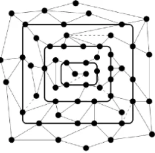
Figure 2: An example of a plane graph C and a tight sequence of 3 concentric cycles in it. Notice that the addition to C of any of the dashed edges makes this collection of cycles non-tight.
Proof. Let x = |T|+1 and y = 2(r+1)·d√xe. From Proposition 1, if tw(C) ≥4.5·y+1, then C contains as a minor a (y × y)-grid . We now observe that the grid contains as subgraphs x pairwise disjoint (2(r + 1) × 2(r + 1))-grids 1,... , x. Note that each , i
{1, . . . , x} contains a sequence of r+1 concentric cycles that, given a minor model of in C, can be used to construct, in linear time, a sequence of r +1 concentric cycles C = {C 0, C 1, ... , C r} in C such that for every i,j {1,.. .,x}, where i =6 j, all cycles in Cj
are in the open exterior of C r.
Note that at least one, say C r, of the cycles in {C1 r ,.. . , Cx r } should contain all the
vertices of T in its open exterior. Let e be any edge of C 0. Let also f be the face of C
that is contained in the open interior of C 0 and is incident to e. Let Jf be the graph
consisting of the vertices and the edges that are incident to f. It is easy to verify that, Jf contains an internally chordless cycle C that contains the edge e. Given C 0, the cycle C can be found in linear time. Notice now that C contains a tight sequence of cycles C0, C1, . . . ,Cr such that C0 = C and where, for h {0, . . . , r}, Ch is in the closed
interior of C h. The result follows as the open exterior of Cr contains the open exterior of C r and therefore contains all vertices in T.
The algorithm runs as follows: it first uses the algorithm of Proposition 2 for k = 4.5 · y. If the algorithm outputs a tree decomposition of C of width at most k, then we are done. Otherwise it outputs a subgraph C0 of C where tw(C0) > k and a tree
decomposition of C0 of width ≤ 2k. We use this tree decomposition in order to find a
minor model of the (y × y)-grid in C0. This can be done in 2k
O(1) = 2(r·√|T |)O(1) · n steps
[image:9.595.219.376.116.271.2]a minor model of in C. We may now use , as explained above, in order to identify, in linear time, the required internally chordless cycle C in C.
Linkages. A linkage in a graph C is a non-empty subgraph
L of C whose connected components are all paths. The paths of a linkage are its connected components and we denote them by 2(L). The terminals of a linkage L are the endpoints of the paths in 2(L), and the pattern of L is the set {{s,t} | 2(L) contains a path from s to tin C}. Two linkages are equivalent if they have the same pattern.
Segments. Let C be a plane graph and let C be a cycle in C whose closed-interior is D. Given a path P in C we say that a subpath P0 of P is a D-segment of P, if P0 is
a non-empty (possibly edgeless) path obtained by intersecting P with D. For a linkage L of C we say that a path P0 is a D-segment of L, if P0 is a D-segment of
[image:10.595.180.414.317.553.2]some path P in 2(L).
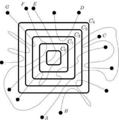
Figure 3: An example of a CL-configuration Q = (C, L) where C contains 5 cycles and
L has 7 paths. Q has 13 segments. Linkage paths A, B, C, D, E, F, and C, contain 2, 2, 2, 1, 1, 2, 3 of these segments respectively. Also the eccentricities of the segments of
CL-configurations. Given a plane graph C, we say that a pair Q = (C, L) is a CL-configuration of C of depth r if C = {C0,. . . , Cr} is a sequence of concentric cycles in C,
L is a linkage of C, and Dr does not contain any terminals of L. A segment of Q is any Dr
-segment of L. The eccentricity of a segment P of Q is the minimum i such that V (Ci flP)
=6
0. A segment of
Q is extremal if it is has eccentricity r. Observe that if C is tight then any extremal segment is a subpath of Cr. Given a cycle Ci E C and a segment P of Q wedefine the i-chords of P as the connected components of P fl
int(
Di) (notice that i-chordsare open arcs). For every i-chord X of P, we define the i-semichords of
P as the connected components of the set X \ Di_1 (notice that i-semichords are
open arcs). Given a segment P that does not have any 0-chord, we define its zone as the connected component of Dr \ P that does not contain the open-interior of D0
[image:11.595.217.380.288.454.2](a zone is an open set).
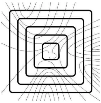
Figure 4: An example of a CL-configuration (C, L) where the linkage L is C-cheap. Only the 5 concentric cycles of C and a cropped part of the linkage L are depicted. Notice that the collection of concentric cycles C is not tight.
A CL-configuration Q = (C, L) is called reduced if the graph L fl C is edgeless. Let
Q = (C, L) be a CL-configuration of C and let E be the set of all edges of the graph
L fl C. We then define C* as the graph obtained if we contract in C all edges in E•.
We also define Q* as the pair (C*, L*) obtained if in L and in the cycles of C we
contract all edges of E•. Notice that Q* is a reduced CL-configuration of C*. We call
Cheap linkages. Let G be a plane graph and Q = (C, L) be a CL-configuration of
G of depth r. We define the function c : {L | L is a linkage of G} N so that
c(L) = | E(L) \ U E(Ci)| . iE{0,...,r}
A linkage L of G is C-cheap, if there is no other CL-configuration Q' = (C, L') such
that L' has the same pattern as L and c(L) > c(L'). Intuitively, the function c defined
above penalizes every edge of the linkage that does not lie on some cycle Ci.
Observation 1. Let Q = (C, L) be a CL-configuration and let (G*, Q* = (C*, L*)) be
the reduced pair of G and Q. Then
If L is C-cheap, then L* is C*-cheap.
[image:12.595.213.374.321.479.2] If C is tight in G, then C* is tight in G*.
Figure 5: An example of a convex CL-configuration (C, L). In the picture, only the 5 cycles in C and a cropped portion of L is depicted.
3.2 Convex configurations
We introduce CL-configurations with particular characteristics that will be useful for the subsequent proofs. We then show that these characteristics are implied by tightness and cheapness.
Convex CL-configurations. A segment P of Q is convex if the following three conditions are satisfied:
(ii) for every i E {1, . . . , r}, the following hold:
a. P has at most one i-chord
b. if P has an i-chord, then P fl Ci−1 =6
0.
c. Each i-chord of P has exactly two i-semichords.
(iii) If P has eccentricity i < r, there is another segment inside the zone of P with eccentricity i + 1.
We say Q is convex if all its segments are convex.
[image:13.595.219.376.305.420.2]Observation 2.
Let Q = (C, L) be a CL-configuration and let (G , Q = (C , L )) be the reduced pair of G and Q. Then Q is convex if and only Q is convex.Figure 6: A visualization of the conditions of Lemma 2.
The proof of the following lemma uses elementary topological arguments.
Lemma 2. Let A
1, A2 be closed disks of R2 where int(A1)flint(A
2) = 0 and such that A1U A2 is also a closed disk. Let A3 = R2 \
int(A
1 U A2) and let Y = bnd(A3) fl A2 and Q =trim(A
1 flA2). Let P be a closed arc of R2 whose endpoints are not in A1 UA2 and suchthat Y fl P =
0
and Q fl P =60.
Thenint(A
1) fl P has at least two connectedcomponents.
Proof. Let q be some point in Q fl P. Let Q0 be an open arc that is a subset of int(A 1)
and has the same endpoints as Y . Notice that q and x belong to different open disks defined by the cycle Q0 U Y . Therefore P should intersect Q0 or Y . As Y fl P = 0, P
intersects Q0
. As Q0 C
int(A
1), int(A1) fl P has at least one connected component.
Assume now that int(A1) fl P has exactly one connected component. Clearly, this
connected component will be an open arc I such that at least one of the endpoints of
I, say q, belongs to Q. Moreover, there is a subset P0 of P that is a closed arc where P 0fl I = 0 and whose endpoints are q and one of x and y, say y. As int(A
exactly one connected component, it holds that
P
'fl
int(L
1) =0. Let
Q
' be an open arcthat is a subset of int(L1) and has the same endpoints as
Y
. Notice thatq
andy
belongto different open disks defined by the cycle
Q
'U Y
. ThereforeP
' should intersect int(L1)or
Y
, a contradiction asP
'c P
andY fl P
= 0.Lemma 3.
LetG
be a plane graph andQ
= (C, L
)be a CL-configuration of
G
whereC
is tight inG
andL
isC
-cheap. ThenQ
is convex.Proof. By Observations 1 and 2, we may assume that
Q
is reduced. Consider any segment ofQ
. We show that it satisfies the three conditions of convexity. Conditions (i) and (ii).b follow directly from the tightness ofC.
Condition (iii) follows from the fact thatL
isC
-cheap. In the rest of the proof we show Conditions (ii).a. and (ii).c. For this, we consider the minimumi E {
0,. . . , r}
such that one of these two conditions is violated. From Condition (i),i
≥
1. LetW
be a segment ofQ
containing ani
-chordX
for which one of Conditions (ii).a, (ii).c is violated.
We now define the set
Q
according to which of the two conditions is violated. We distinguish two cases:Case 1. Condition (ii).c is violated. From Condition (ii).b,
X
\Di_1 contains more thantwo
i
-semichords ofX
. LetJ
1 be the biconnected outerplanar graph defined by theunion of Ci_1 and the
i
-semichords ofX
that do not have an endpoint onC
i. As thereare at least three
i
-semichords inX
,J
1 has at least one internal edge and therefore atleast two simplicial faces. Moreover there are exactly two
i
-semichords ofX
, sayK
1,K
2, that have an endpoint inC
i andK
1 andK
2 belong to the same, sayF
', face ofJ
1.Let L2 be the closure of a simplicial face of
J
1 that is notF
'.Case 2. Condition (ii).c holds while Condition (ii).a is violated. Let
J
2 be thebicon-nected outerplanar graph defined by the union of Ci_1 and the connected components
of
W \ D
i_1 that do not contain endpoints ofW
in their boundary. Notice that the restof the connected components of
W \ D
i_1 are exactly two, sayK
1 andK
2. Notice thatK
1 andK
2 are subsets of the same face, sayF
', ofJ
2. As there are at least twoi
-chordsin
W
,J
2 contains at least one internal edge and therefore at least two simplicial faces.Let L2 be the closure of a simplicial face of
J
2 that is notF
'.In both of the above cases, we set L1 =
D
i_1, L3 =R
2\
int(L
1U
L2),Y
=bnd(L
3)fl
L2, andQ
=trim(L
1fl
L2). Notice thatY
=bnd(L
2)\ Q
, thereforeY c W
.We claim that
L fl Q
=6
0. Suppose not. We consider
W
' as the path inW U Q
thatcontains
Q
as a subset and has the same endpoints asW
. Then,L
' = (L \ W
)U W
' isa linkage, equivalent to
L
, wherec
(L
')< c
(L
), a contradiction to the fact thatL
isC
-cheap. We just proved that
LflQ
=6
0 which in turn implies that
L
contains a segmentP
for whichP fl Q
=6
0. We distinguish two cases:
Figure 7: The two cases of the proof of Lemma 3. In the left part is depicted an i-chord X
that has 6 i-semichords and in the right part is depicted a segment W and the way it crosses the cycles Di and Di−1. In the figure on the right the segment W has 7 i-chords and
14 i-semichords.
has at least two (i − 1)-chords. If i > 1, then Condition (ii).a is violated for i − 1, which contradicts the choice of i. If i = 1, then P has at least one 0-chord, which violates Condition (i), that, as explained at the beginning of the proof, holds for every segment of Q.
Case B. W = P. Recall that Y c W therefore Y c P. Let p1 and p2 be the endpoints
of Q. As Q is reduced there exists two disjoint closed arcs Z1 and Z2 with endpoints
p1, p01 and p2, p02 respectively, such that
pi is an endpoint of Zi, i E {1, 2}. Zi c
clos
(Q),i E {1,2}, and P fl Zi = {pi},i E {1,2}.Consider also a closed arc Y0 that is a subset of
int
(2) U {p01,p0 2} that does not
intersect L and whose endpoints are p0
1 and p02. Let now 01= 1, let 02 be the closed
disk defined by the cycle
clos
(Q \ (Z1 U Z2)) U Y 0that is a subset of 2. Let also 0 3 =R
2 \int
( 01 U 0 2) and Q0 =
trim
( 01 fl 02). As Y 0 does not intersect L, we obtain Y 0fl P =
o
. Observe that Z1, Q0, Z2 form a partition of Q. As Q fl P =6o
and (Zi \ {pi}) fl P=
o
,i E {1,2}, we conclude that Q0 fl P =6o
.By applying Lemma 2,
int
( 01)flP has at least two connected components. Therefore P
3.3 Bounding the number of extremal segments
In this subsection we prove that the number of extremal segments is bounded by a linear function of the number of linkage paths.
Out-segments, hairs, and flying hairs.
Let G be a plane graph and Q = (C, L) be a CL-configuration of G of depth r. An out-segment of L is a subpath P' of a pathin P(L) such that the endpoints of P' are in Cr and the internal vertices of P' are not in
Dr. A hair of L is a subpath P' of a path in P(L) such that one endpoint of P' is in Cr,
the other is a terminal of L, and the internal vertices of P' are not in Dr. A flying hair
of L is a path in P(L) that does not intersect Cr.
Given a linkage L of G and a closed disk D of R2 whose boundary is a cycle of G, we define outD(L) to be the graph obtained from the graph (L
bnd(
D)) \int(
D) afterdissolving all vertices of degree 2. For example outDr(L) is a plane graph consisting of
the out-segments, the hairs, the flying hairs of L, and what results from Cr after
dissolving its vertices of degree 2 that do not belong in L. Let f be a face of outDr(L)
that is different from int(Dr). We say that f is a cave of outDr(L) if the union of the
out-segments and extremal out-segments in the boundary of f is a connected set. Recall that a segment of Q is extremal if it is has eccentricity r, i.e., it is a subpath of Cr.
Given a plane graph G, we say that two edges e1 and e1 are cyclically adjacent if
they have a common endpoint x and appear consecutively in the cyclic ordering of the edges incident to x, as defined by the embedding of G. A subset E of E(G) is cyclically connected if for every two edges e and e' in E there exists a sequence of
edges e1, . . . , er E where e1 = e, er = e' and for each i {1, . . . , r − 1} ei and ei±1 are cyclically adjacent.
Let Q = (C, L) be a CL-configuration. We say that Q is touch-free if for every path P of L, the number of the connected components of P Cr is not 1.
Lemma 4. Let
G be a plane graph and Q = (C, L) be a touch-free CL-configuration of G where C is tight in G and L is C-cheap. The number of extremal segments of Qis at most 2 · |P(L)| −2.
Proof. Let (G*, Q* = (C*, L*)) be the reduced pair of G and Q. Notice that, by
Ob-servation 1, C* is tight in G and L* is C*-cheap. Moreover, it is easy to see that Q* is
touch-free and Q and Q* have the same number of extremal segments which are all
trivial paths (i.e., paths consisting of only one vertex). Therefore, it is sufficient to prove that the lemma holds for Q*. Let be the number of extremal segments of Q*.
Let J = outDr(L
*) and k = |P(L*)|. Notice that the number of extremal segments of
Q* is equal to the number of vertices of degree 4 in J.
The terminals of L* are partitioned in three families
invading terminals T1: these are endpoints of hairs whose non terminal
endpoint has degree 3 in J.
bouncing terminals T2: these are endpoints of hairs whose non terminal
endpoint has degree 4 in J.
A hair containing an invading and bouncing terminal is called invading and bouncing hair respectively.
Recall that |T0| + |T1| + |T2| = 2k.
Claim 1. The number of caves of J is at most the number of invading terminals. Proof of claim 1. Clearly, a hair cannot be in the common boundary of two caves. Therefore it is enough to prove that the set obtained by the union of a cave f and its boundary contains at least one invading hair. Suppose this is not true. Consider the open arc R obtained if we remove from bnd(f) all the points that belong to out-segments. Clearly, R results from a subpath R+ of C*
r after removing its endpoints,
i.e., R = trim(R+).
Notice that because f is a cave, R is a non-empty connected subset of C* r.
Moreover, R n L* is non-empty, otherwise L*' = (L* \ (bnd(f)) U R is also a linkage with
the same pattern as L* where c(L*') < c(L*), a contradiction to the fact that L* is C*
-cheap. Let Y be a connected component of R n L*. As Q* is reduced, Y consists of a
single vertex y in the open set R. Notice that Y is a subpath of a segment Y' of Q*. We
claim that Y' is not extremal. Suppose to the contrary that Y' is extremal. Then Y ' = Y
and there should be two distinct out-segments that have y as a common endpoint. This contradicts the fact that y E R.
By Lemma 3, Q* is convex, therefore one of the endpoints of the non-extremal
segment Y ' is y and thus is in R as well. This means that y is the endpoint of one
out-segment which again contradicts the fact that y E R. This completes the proof of Claim 1.
Let J— be the graph obtained from J by removing all hairs and notice that J— is a biconnected outerplanar graph. Let S be the set of vertices of J— that have degree 4. Notice that, because Q* is touch-free, |S| is equal to the number of vertices of J that
have degree 4 minus the number of bouncing terminals. Therefore,
= |T2| + |S|. (1)
Notice that if we remove from J— all the edges of C*
r, the resulting graph is a forest
whose connected components are paths. Observe that none of these paths is a trivial path because Q* is touch-free. We denote by ( Ψ the number of connected components
of . Let F be the set of faces of J— that are different from D*
r. F is partitioned into the
faces that are caves, namely F1 and the non-cave faces, namely F0. By the Claim 1,
Figure 8: Examples of the graphs J and J− in the proof of Lemma 4 (the outer face in the picture corresponds to the interior of Dr). The faces that are caves contain the
word cave. FH: flying hair, BH: bouncing hair, IH: invading hair. The forest = J−\E(Cr)
has 6 edges and 4 connected components. The weak dual T of J− is depicted with dashed lines. The large white square vertices are the rich vertices of T.
To complete the proof, it is enough to show that
|S| ≤ |T1| −2 (2)
Indeed the truth of (2) along with (1), would imply that p is at most |T2| + |S| ≤ |T2|
+ |T1| −2 ≤ |T| −2 = 2k −2.
We now return to the proof of (2). For this, we need two more claims.
Claim 2: |F0| ≤ ( Ψ −1.
Proof. We use induction on ( Ψ. Let K1,... , K( Ψ be the connected components of . If ( ) = 1 then all faces in F are caves, therefore |F0| = 0 and we are done.
Assume now that contains at least two connected components.
We assert that there exists at least one connected component Kh of with the
property that only one non-cave face of J− contains edges of Kh in its boundary. To see this, consider the weak dual T of J−. Recall that, as J− is biconnected, T is a tree. Let K i be the subtree of T containing the duals of the edges in E(Ki), i {1,. . . , ( Ψ}, and observe that E(K1), . . . , E(K ( ΨΨ is a partition of E(T) into ( Ψ cyclically connected sets.
We say that a vertex of T is rich if it is incident with edges in more than one members of
{K 1,. . . , K ( Ψ}, otherwise it is called poor (see Figure 8). Notice that a vertex of T is
rich if and only if its dual face in J− is a non-cave. We call a subtree K i peripheral if V (K
i ) contains at most one rich vertex of T. Notice that the claimed property for a component
in {K1,. . . , K( Ψ} is equivalent to the existence of a peripheral subtree in {K 1, . . . , K
( Ψ}. To prove that such a peripheral subtree exists, consider a path P in T intersecting the vertex sets of a maximum number of members of
W1, ... ,K (4Ψ1. Let e be the first edge of P and let Kh be the unique subtree whose
edge set contains e. Because of the maximality of the choice of P, V (Kh) contains
exactly one rich vertex vh, therefore Kh is peripheral and the assertion follows. We
denote by fh the non-cave face of J−that is the dual of vh.
Let II−be the outerplanar graph obtained from J−after removing the edges of Kh. Notice that this removal results in the unification of all faces that are incident to the edges of Kh, including fh, to a single face f+. By the inductive hypothesis the number of
non-cave faces of II−is at most ( Ψ—2. Adding back the edges of Kh in J−restores fh as a distinct non-cave face of J−. If f+ was a non-cave of II−then |F0| is equal to the
number of non-cave faces of II−, else |F0| is one more than this number. In any case,
|F0| < ( Ψ —1, and the claim follows.
Claim 3: |V ( Ψ| < |T1| + 2 - ( Ψ —2.
Proof. Let T be the weak dual of J−. Observe that |F0| + |F1| = |F| = |V (T)| = |E(T)|
+1 = |E( Ψ| +1 = |V ( Ψ| — ( Ψ +1. Therefore |V ( Ψ| = |F0| + |F1| + ( Ψ —1.
Recall that, by Claim 1, |F1| < |T1| and, taking into account Claim 2, we conclude
that |V ( Ψ| < |T1| + 2 • ( Ψ —2. Claim 3 follows.
Notice now that a vertex of J− has degree 4 iff it is an internal vertex of some path in . Therefore, as all connected components of are non-trivial paths, it holds that |V ( Ψ| = |S| + |L( Ψ| = |S| + 2 • ( Ψ, where L( Ψ is the set of leaves of . By Claim 3,
|S| + 2 - ( Ψ = |V ( Ψ| < |T1| + 2 - ( Ψ —2 = |S| < |T1| —2.
Therefore, (2) holds and this completes the proof of the lemma.
3.4 Bounding the number and size of segment types
In this section we introduce the notion of segment type that partitions the segments into classes of mutually “parallel” segments. We next prove that, in the light of the results of the previous section, the number of these classes is bounded by a linear function of the number k of linkage paths. In Subsections 3.5 and 3.6 we show that if one of these equivalence classes has size more than 2k, then an equivalent cheaper linkage can be
found. All these facts will be employed in the culminating Subsection 3.7 in order to prove that a cheap linkage cannot go very “deep” into the cycles of a cheap CL -configuration. That way we will be able to quantify the depth at which an irrelevant vertex is guaranteed to exist.
Types of segments. Let G be a plane graph and let Q = (C, L) be a convex CL-configuration of G. Let S1, S2 be two segments of Q and let P and P0 be the two paths
on Cr connecting an endpoint of S1 with an endpoint of S2 and passing through no
(1) no segment of Q has both endpoints on P.
(2) no segment of Q has both endpoints on P0.
(3) the closed-interior of the cycle P U S1 U P0 U S2 does not contain the disk D0.
A type of segment is an equivalence class of segments of Q under the relation k .
Given a linkage L of G and a closed disk D of R2 whose boundary is a cycle of
G, we define
inD(
L) to be the graph obtained from (L Ubnd(
D)) fl D after dissolving all vertices of degree 2.Notice that
inD
T(L) is the biconnected outerplanar graph formed if we dissolve allvertices of degree 2 in the graph that is formed by the union of Cr and the segments of
Q. As Q is convex, one of the faces of inDT(L) contains the interior of D0 and we call this
face central face. We define the segment tree of Q, denoted by T(Q), as follows.
Let T − be the weak dual of inDT(L) rooted at the vertex that is the dual of the
central face.
Let Q be the set of leaves of T −. For each vertex l E Q do the following: Notice first that l is the dual of a face l of
inD
T(L). Let W1,... , W l be the extremal segments in the boundary of l (notice that, by the convexity of Q, for every l, l ≥ 1). Then, for each i E {1,. . . , l}, create a new leaf wi corresponding to the extremal segment Wi and make it adjacent to l.The height of T(Q) is the maximum distance from its root to its leaves. The real height of T(Q) is the maximum number of internal vertices of degree at least 3 in a path from its root to its leaves plus one. The dilation of T(Q) is the maximum length of a path all whose internal vertices have degree 2 and are different from the root.
Observation 3. Let
G be a plane graph and let Q = (C, L) be a convex CL-configuration of G. Then the dilation of T(Q) is equal to the maximum cardinality of an equivalence class of ||.Observation 4.
Let G be a plane graph and let Q = (C, L) be a convex CL-configuration of G. Then the height of T(Q) is upper bounded by the dilation of T(Q) multiplied by the real height of T(Q).The following lemma is an immediate consequence of Lemma 4 and the definition of a segment tree. The condition that L fl Cr =6
0 simply requires that the CL-configuration
that we consider is non-trivial in the sense that the linkage L enters the closed disk Dr.
Lemma 5. Let
G be a plane graph and Q = (C, L) be a touch-free CL-configuration of G where C is tight in G, L is C-cheap, and L fl Cr =60. Then
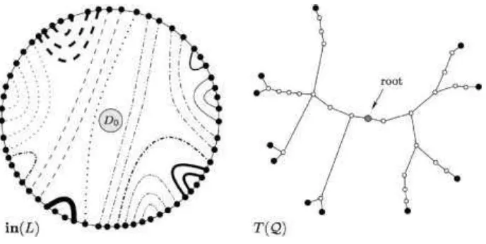
Q is convex and theFigure 9: The graph
in
Dr(L) for some convex CL-configuration Q = (C, L) and the treeT(Q). Internal edges in
in
Dr(L) of the same type are drawn as lines of the same type.Q has 11 extremal segments, as many as the leaves of T(Q). The relation k has 19 equivalent classes. The dilation of T(Q) is 4, its height is 8 and its real height is 4.
Proof. Certainly, the convexity of Q follows directly from Lemma 3. We examine the non-trivial case where T(Q) contains at least one edge. We first claim that |P(L)| ≥2. Assume to the contrary that L consists of a single path P. As Q is convex and L Cr =6
0
, Q has at least one extremal segment. Suppose now that Q has more than one extremal segment all of which are connected components of Cr P. Let P1 and P2 bethe closures of the connected components of L \ Dr that contain the terminals of P. Let
pi V (Cr) be the endpoint of Pi that is not a terminal, i {1, 2}. Let also P' be any path
in Crbetween p1 and p2. Notice now that P1 P' P2 is a cheaper linkage with the
same pattern as L, a contradiction to the fact that L is C-cheap. Therefore we conclude that Q has exactly one extremal segment, which contradicts the fact that Q is touch-free. This completes the proof that |P(L)| ≥2.
Recall that, by the construction of T(Q) there is a 1–1 correspondence between the leaves of T(Q) and the extremal segments of Q. From Lemma 4, T(Q) has at most 2 · |P(L)| −2 leaves. Also T(Q) has at least 2 leaves, because Q is touch-free. It is known that the number of internal vertices of degree ≥3 in a tree with r ≥2 leaves is at most
r −2. Therefore, T(Q) has at most 2· |P(L)| −4 internal vertices of degree ≥ 3. Therefore the real height of T(Q) is at most 2 · |P(L)| −3.
3.5 Tidy grids in convex configurations
Topological minors. We say that a graph
H is a topological minor of a graph C if there exists an injective function 0 : V (H) V (C) and a function 1 mapping theedges of H to paths of C such that
for every edge {x,y} E E(H), 1({x,y}) is a path between 0(x) and 0(y).
if two paths in 1(E(H)) have a common vertex, then this vertex should be an
endpoint of both paths.
Given the pair ( 0, 1), we say that H is a topological minor of C via ( 0, 1).
Tilted grids and
L-tidy grids. Let
C be a graph. A tilted grid of C is a pair U = (X, Z) where X = {X1,... , Xr} and Z = {Z1,. . . , Zr} are both collections of rvertex-disjoint paths of C such that
for each i,j E {1,... ,r} Ii,j = Xi fl Zj is a (possibly edgeless) path of C,
for i E {1,.. . ,r} the subpaths Ii,1,Ii,2, . . . , Ii,r appear in this order in Xi.
for j E {1,. . . , r} the subpaths I1,j, I2,j,. . . , Ir,j appear in this order in Zj.
E(I1,1) = E(I1,r) = E(Ir,r) = E(Ir,1) = 0, Let
U
CU = ( Xi) ( U Zi)i {1,...,r} i {1,...,r}
and let C U be the graph taken from the graph after contracting all edges in U(i,j) {1,...,r}2 Ii,j. Then C U contains the (r x r)-grid F as a topological minor
via a pair ( 0, 1) such that
A. the upper left (resp. upper right, down right, down left) corner of F is mapped via 0 to the (single) endpoint of I1,1 (resp. I1,r, Ir,r, and Ir,1).
B. Ue E( Ψ 1(e) = C U (this makes C U to be a subdivision of F).
We call the subgraph CU of C realization of the tilted grid U and the graph C U
representation of U. We treat both CU and C U as plane graphs. We also refer to the cardinality r of X (or Z) as the capacity of U. The perimeter of CU is the cycle X1
Z1 Xr Zr. Given a graph C and a linkage L of C we say that a tilted grid U = (X,
Z) of C is an L-tidy tilted grid of C if DU fl L = Z where DU is the closed-interior of the perimeter of CU.
Figure 10: A visualisation of the proof of Lemma 6. It holds that a1 = 0 and a5 = 4, m = 5, m' = 3. The two shadowed regions indicate the two connencted components
of DS fl AC.
Proof. Let C = {C0,... , Cr} and let S = {S1,. . . , Sm}. For each i E {1,.. . , m}, let ai be
the eccentricity of Si and let amax = max{ai | i E {1, . . . , m}} and amin = min{ai | i E
{1,.. . , m}}. Convexity allows us to assume that S1, . . . , Sm are ordered in a way
that
a1 = amin,
am = amax, and
for all i E {1,...,m − 1}, ai+1 = ai + 1.
for all i E {1,.. . , m}, Ii, i = Si fl C i is a subpath of C i.
Let m' = [m 2 e and let x, x' (resp. y, y') be the endpoints of the path S1 (resp. Sm') such that the one of the two (x, y)-paths (resp. (x', y')-paths) in Cr contains both x', y' (x, y)
and the other, say P (resp. P'), contains none of them. Let DS be the closed-interior of
C max−(m,−1) and C max. Let be any of the two connected components of DS n AC.
We now consider the graph
(L U uC) n .
It is now easy to verify that the above graph is the realization GU of a tilted grid U =
(X, Z) of capacity m0, where the paths in X are the portions of the cycles
C max−(m,−1), . . ., C max cropped by , while the paths in Z are the portions of the
paths in {S1, . . . , Sm,} cropped by
(see Figure 10Ψ. As S is an
equivalence class of k, it follows that U is L-tidy, as required.
3.6 Replacing
linkages by cheaper ones
In this section we prove that a linkage L of k paths can be rerouted to a cheaper one, given the existence of an L-tidy tilted grid of capacity greater than 2k. Given that L is a
cheap linkage, this will imply an exponential upper bound on the capacity of an L-tidy tilted grid.
Let G be a plane graph and let L be a linkage in G. Let also D be a closed disk in the surface where G is embedded. We say that L crosses vertically D if the outerplanar graph defined by the boundary of D and L n D has exactly two simplicial faces. This naturally partitions the vertices of
bnd(
D)nL into the up and down ones. The following proposition is implicit in the proof of Theorem 2 in [3] (see the derivation of the unique claim in the proof of the former theorem). See also [8] for related results.Proposition 3.
Let G be a plane graph and let D be a closed disk and a linkage Lof G of order k that crosses D vertically. Let also L n D consist of r > 2k lines. Then
there is a collection Ar of strictly less than r mutually non-crossing lines in D each connecting two points of bnd(D) n L, such that there exists some linkage R that is a subgraph of L \
int(
D) such that RUUAr is a linkage of the graph (G \ D)UUAr that is equivalent to L.Lemma 7. Let
k, k0, be integers such that 0 < < k0 < k. Let be a (k x k0)-grid and let {pu
1p , . . . ,p up} (resp. {pdown
1 , . . . ,down}) be vertices of the higher (resp. lower)
horizontal line arranged as they appear in it from left to right. Then the grid contains pairwise disjoint paths P1, . . . , P such that, for every h E [ ], the endpoints of Ph are phup
and phdown .
Proof. W e use induction on . Clearly the lemma is obvious when = 0. Let (i, j) E [k]2such that p up (resp. p d o wn) is the i-th (resp. j-th) vertex of
the higher (lower) horizontal line counting from left to right. W e examine first the case where i > j. Let P be the path created by starting from p up,
moving k0 — 1 edges down, and then i — j edges to the left. For h E [ —
1] let P (d o wn) 0 be the path created by starting from pdown h and h
moving one edge up (clearly, P (down)0 consists of a single edge). We also denote by
Figure 11: An example of the proof of Lemma 7, where k = 16, k0 = 11, and = 5. The white vertices of the higher (resp. lower) horizontal line are the vertices in {pup
1 , . . . , pup 5 }
(resp. {pdown 1 , . . ., pdown 5 }).
p(down)0
the other endpoint of P(down)0.We now define as the subgrid of that occurs i
from after removing its lower horizontal line and, for every h [i,k], its h-th vertical line. By construction, none of the edges or vertices of P belongs in 0. Notice also
that the higher (resp. lowerΨ horizontal line of 0 contains all vertices in {pup
1 , . . . , pup 1 }
(resp. {p1(down)0 (down)0}Ψ. From the induction hypothesis, 0 contains −1 pairwise
disjoint paths P0
1, . . . , P0 −1 such that for every h [ − 1], the endpoints of Ph are puhp and p(down)0 . It is now easy to verify that P 1 0 P (down)0 , . . . , P 0 −1 P (down)0
−1 , P is the
h 1
required collection of pairwise disjoint paths. For the case where i < j, just reverse the same grid upside down and the proof is identical (see Figure 11).
Lemma 8. Let be a (k × k)-grid embedded in the plane and
assume that the vertices of its outer cycle, arranged in clockwise order, are:
up{v
1 , . . . ,vk up, v2 right, . . . ,vkrigh1t, vdown
k , . . . ,vdown 1 , vleft k−1, . . . ,vl2eft, ,v 1 }.
Let also H be a graph whose vertices have degree 0 or 1 and they can be cyclically arranged in clockwise order as
{xup 1 , . . . ,xup k ,xdown k , . . . ,xdown 1 ,xup
1 }
such that if we add to H the edges formed by pairs of consecutive vertices in this cyclic ordering, the resulting graph H+ is outerplanar. Let V 1 be the vertices of H that have degree 1 and let H1 = H[V 1]. Then H1is a topological minor of via some pair ( 0, 1), satisfying the following properties:
i ) = vup
2. 00(xdown
i ) = vd o w n
i , i {1, . . . , k} V 1.
Proof. Let U = {xup
1, . . . ,xkup} V 1 and D = V 1. We define 00 as
in the statement of the lemma. In the rest of the proof we provide the definition of 01.
We partition the edges of H1 into three sets: the upper edges EU that connect vertices
in U, the down edges EL that connect vertices in D, and the crosssing edges EC that have one endpoint in U and one in D. As |V (H1)| ≤2k we obtain that |E(H1)| ≤ k and
therefore |EU| + |ED| + |EC| = |E(H1)| ≤ k. We set = |EC|.
We recursively define the depth of an edge {xiup, xup
j } in EU as follows: it is 0 if there is no edge of EU with an endpoint in {xup
i+1, . . . , xup
j−1} and is i > 0 if the maximum
depth of an edge with an endpoint in {xup
i+1, . . . , xup
j−1} is i −1. The depth of an edge
{xdown i , xdown
j} is defined analogously. It directly follows, by the definition of depth that:
qup = max{depth(e) | e EU} + 1 ≤ |EU| (3)
qdown = max{depth(e) | e ED} + 1 ≤ |ED| (4)
[image:27.595.94.505.356.556.2]We now continue with the definition of 01 as follows:
Figure 12: An example of the proof of Lemma 8. On the left, the (16 × 16)-grid G is depicted along with the way the graph H (depicted on the right) is (partially) routed in it. In the figure qu
p = 3, qdown = 2, k
'
= 11, and = 5.• for every edge e = {xiup, xup
j } in EU, of depth l and such that i < j, let 01(e) be
the path defined if we start in the grid G from viup, move l steps down, then j −
i steps to the right, and finally move l steps up to the vertex vup
• for every edge e = {xdown
i , xdown
j } in ED, of depth l and such that i < j, let 01(e) be
the path defined if we start in the grid G from vdown
i , move l steps up, then
j — i steps to the right, and finally move l steps down to the vertex vdown
j .
Notice that the above two steps define the values of 01 for all the upper and down edges.
The construction guarantees that all paths in 01(EU U ED) are mutually non-crossing. Also,
the distance between 00(UΨ and some horizontal line of that contains edges of the
images of the upper edges is max{depth(e) | e E EU} that, from (3), is equal to qu p —1.
Symmetrically, using (4) instead of (3), the distance between 00(D) and the horizontal
lines of that contain edges of the images of the down edges is equal to qdown —1. As a
consequence, the graph
0 = \ {x E V ( Ψ |
dist
(x, 00(U)) < qup Vdist
(x, 00(D)) < qdown}is a (k x k0)-grid 0, where k0 = k —(qu
p + qdown), whose vertices do not appear in any of
the paths in 01(EU U ED). Given a crossing edge e = {xup i ,xdown
j } E EC, we define the path P up
e as the subpath of created if we start from xiup and then go qup steps down.
Similarly, we define Pedownas the subpath of created if we start from x
down
j and then go qdown steps up. Notice that each of the paths P e up (resp. P down
e ) share only one vertex,
say pup
e (resp. pedown Ψ, with 0 that is one of their endpoints (these endpoints are depicted as white vertices in the example of Figure 12). We use the notation {pu
1p, . . . ,pup} (resp. {pdown 1 , . . . ,p down,
1) for the vertices of the set {peup | e E EC} (resp. {pedown | e E EC})
such that, for every h E [ ], there exists an e E EC such that pu
hp is an endpoint of Peupand pdown
h is an endpoint of Pedown. We also agree that the vertices in {pu1p, . . . ,p up}
(resp. ,p down}) are ordered as they appear from left to right in the upper
(lowerΨ horizontal line of 0 (this is possible because of the outeplanarity of H+).
Notice that = |E(H1)| —(|EU| + |ED|) < k —(|EU| + |ED|) which by (3) and (4)
implies that < k0.
As < k0 < k, we can now apply Lemma 7 on 0, {pu
1p, . . . ,p up} and {pdown
1 , . . .,p down} and obtain a collection {Pe | e E EC} of pairwise disjoint paths in
0 between the vertices of {p
eup | e E EC} and the vertices of {pdown
e |e E
EC}. It is now easy to verify that {P up
e U Pe u Pedown | e E EC} is a collection of vertex disjoint
paths between U and D. We can now complete the definition of 01 for the crossing
edges of H by setting, for each e E EC, 0(e) = P up
e U Pe U Pedown. By the
above construction it is clear that (01, 02) provides the claimed
topological isomorphism.
Lemma 9.
Let G be a graph with alinkage L consisting of k paths. Let also U = (X, Z) be an L-tidy tilted grid of G with capacity m. Let also be the closed-interior of the perimeter of GU. If m > 2k, then G
contains a linkage L0 such that
3. |E(UZ n L0)| < |E(UZ n L)|.
Proof. We use the notation X = {X1,. . . , Xm} and Z = {Z1,. . . , Zm}. Let GU be the
realization of U in G and let G (resp. L) be the graph (resp. linkage) obtained from
G (resp. L) if we contract all edges in the paths of 1j(i,j) {1,...,r}2 Ii,j, where Ii,j = Xi n Zj,
i, j E {1, . . . , m}. We also define X and Z by applying the same contractions to their paths. Notice that U = (X , Z ) is an L-tidy tilted grid of G with capacity m and that the lemma follows if we find a linkage L0 such that the above three conditions
are true for A, L , L0 , and Z, where A is the closed-interior of the perimeter of G U
(recall that GU is the representation of U that is isomorphic to GU.).
Let G− = (G \ A ) U UZ and apply Proposition 3 on G−, A , and L. Let Ar be a collection of strictly less than m mutually non-crossing lines in D each connecting two points of
bnd(A )
nL and a linkage R C L \int(A ) such that
L0 = RUUAr is alinkage of the graph (G \A )UUAr that is equivalent to L. Let H = (L0nA )U(L n
bnd(A )). Notice that in
H, the set V (L0 nA ) contains the vertices of Hof degree 1 while the rest of the vertices of H have degree 0 and all edges of H
have their endpoints in V (L0 nA ). Recall that the (m x m)-grid is a topological
minor of GU via some pair ( 0, 1) satisfying the conditions A and B in the definition
of tilted grid.
We are now in position to apply Lemma 8 for the (m x m)-grid and H. We obtain that H1 = L0 n A is a topological minor of via some pair (00, 01). We now
define the graph
[
L = E(01(e)).e E(H1)
Notice that L is a subgraph of . We also define the graph
Q = U 1 (e)
e E(L)
which, in turn, is a subgraph of GU. Observe that L0 = R U Q is a linkage of G
that is equivalent to L. This proves Condition 1. Condition 2 follows from the fact that R C L \
int(A ). Notice now that, as
|Ar| < m, E(UZ n Q) is a proper subset of E(UZ ). By construction of L0 , it holds that E(UZ n L0 ) = E(UZ n Q). Moreover,as U = (X , Z ) is an L-tidy tilted grid of G, it follows
that E(UZ ) = E(UZ n L ). Therefore, Condition 3 follows.
3.7 Existence of an irrelevant vertex
We now bring together all results from the previous subsections in order to prove Theorem 1.
Lemma 10. There exists an algorithm that, given an instance (
G,P = {(si, ti) E V(G)2, i E {1, . . . , k}}) of PDPP, either outputs a tree-decomposition of G of width
at most 9 • (k • 2k+2 + 1) • V2k + 11 or outputs an irrelevant vertex x E V (G) for (G,
Proof. Let T = {s1,... ,sk,t1,... ,tk}. By applying the algorithm of Lemma 1, for r =
k.2k+2 either we output a tree-decomposition of G of width at most 9(r+1).F√2k _ +11)
or we find an internally chordless cycle C of G such that G contains a tight sequence of cycles C = {C0, . . . , Cr} in G where C0 = C and all vertices of T are in the open exterior
of Cr. From Lemma 1, this can be done in 2(r·√|T|)O(1) . n = 22O(k) . n steps.
Assume that G has a linkage whose pattern is P and, among all such linkages, let L be a C-cheap one. Our aim is to prove that V (L C0) = 0, i.e., we may pick x to be any of the vertices in D0.
First, we can assume that k ≥ 2. Otherwise, if k = 1, the fact that L is C-cheap, implies that L Dr−1 = 0 L D0 = 0 and we are done.
For every i {0, . . . , r}, we define Q(i) = (C(i), L(i)) where C(i) = {C0, . . . , Ci} and L(i) is
the subgraph of L consisting of the union of the connected components of L that have common points with Di. As r + 1 > k, at least one of Q(i), i {0, . . . , r} is touch-free.
Let Q0 = (C0, L0) be the touch-free CL-configuration in {Q(1), . . . , Q(r)} of the highest
index, say h. In other words, C0 = C(h) and L0 = L(h). Moreover, C0 is tight in G and L0 is C0-cheap. Let k0 be the number of connected components of L0. We set d = r − h and
observe that k0≤ k − d, while C0 has r0 = r + 1 − d > 0 concentric cycles. Again, we
assume that k0≥2 as, otherwise, the fact that L0 is C0-cheap implies that L0 Dr
' −1 = 0 L0 D0 = 0 and we are done. Therefore 0 ≤ d ≤ k −2.
As C0 is tight in G and L0 is C0-cheap, by Lemma 3, Q0 is convex. To prove that V (L C0) = 0 it is enough to show that all segments of Q have positive eccentricity and for
this it is sufficient to prove that all segments of Q0 have positive eccentricity. Assume to
the contrary that some segment P0 of Q0 has eccentricity 0. Then, from the third
condition in the definition of convexity we can derive the existence of a sequence P0, . .
. , Pr'−1 of segments such that for each i {0, . . . , r0−1}, Pi+1 is inside the zone of Pi.
This implies the existence in the segment tree T(Q0) of a path of length r0 from its root
to one of its leaves, therefore T(Q0) has height r0. By Lemma 5, the real height of T(Q0)
is at most 2k0−3. By Observation 4, the dilation of T(Q0) is at least
2k'' 3 ≥k·2k 2k−
+2−2d 2d k 2.k+k 2 = 2k+1. By Observation 3 and Lemma 6, G contains an L0-tidy tilted grid U = (X, Z) of capacity > 2k. From Lemma 9, G contains another linkage
L00 with the same pattern as L0 and such that c(L00) < c(L0), a contradiction to the fact
that L0 is C0-cheap.
Since V (L C0) = 0, any vertex of G in the closed-interior of C0 is
irrelevant.