Advances in nowcasting influenza-like illness rates using search query logs

Advances in nowcasting influenza-like

illness rates using search query logs

The Harvard community has made this

article openly available. Please share how

this access benefits you. Your story matters

Citation

Lampos, Vasileios, Andrew C. Miller, Steve Crossan, and Christian

Stefansen. 2015. “Advances in nowcasting influenza-like illness

rates using search query logs.” Scientific Reports 5 (1): 12760.

doi:10.1038/srep12760. http://dx.doi.org/10.1038/srep12760.

Published Version

doi:10.1038/srep12760

Citable link

http://nrs.harvard.edu/urn-3:HUL.InstRepos:21461274

Terms of Use

This article was downloaded from Harvard University’s DASH

repository, and is made available under the terms and conditions

applicable to Other Posted Material, as set forth at

http://

www.nature.com/scientificreports

Advances in nowcasting

influenza-like illness rates using search query

logs

Vasileios Lampos1,2_{, Andrew C. Miller}2,3_{, Steve Crossan}2 _{& Christian Stefansen}2

User-generated content can assist epidemiological surveillance in the early detection and prevalence estimation of infectious diseases, such as influenza. Google Flu Trends embodies the first public platform for transforming search queries to indications about the current state of flu in various places all over the world. However, the original model significantly mispredicted influenza-like illness rates in the US during the 2012–13 flu season. In this work, we build on the previous modeling attempt, proposing substantial improvements. Firstly, we investigate the performance of a widely used linear regularized regression solver, known as the Elastic Net. Then, we expand on this model by incorporating the queries selected by the Elastic Net into a nonlinear regression framework, based on a composite Gaussian Process. Finally, we augment the query-only predictions with an autoregressive model, injecting prior knowledge about the disease. We assess predictive performance using five consecutive flu seasons spanning from 2008 to 2013 and qualitatively explain certain shortcomings of the previous approach. Our results indicate that a nonlinear query modeling approach delivers the lowest cumulative nowcasting error, and also suggest that query information significantly improves autoregressive inferences, obtaining state-of-the-art performance.

User-generated content published on or submitted to online platforms has been the main source of infor-mation in various recent research efforts1–3_{. It has been shown that large data sets of social media posts} and search engine queries contain signals representative of real-life patterns and are therefore indicative of social phenomena in a variety of domains, including politics4,5_{, finance}6_{, commerce}7,8_{, and health}9,10_. Focusing on health-oriented applications, early research efforts have provided empirical evidence of the informativeness of website11 _{and search engine logs}9,12,13 _{for predicting influenza-like illness (ILI) rates.} Google Flu Trends (GFT; http://www.google.org/flutrends)13_{, in particular, is the first real-time system to} apply such methods in practice over a considerable number of countries and a large time span. Similar results were derived through the application of simple10,14 _{or more elaborate}15–17 _{natural language} pro-cessing techniques to content published on the micro-blogging, social networking platform of Twitter.

Data driven estimates can undoubtedly complement current sentinel surveillance systems. One of the original motivations for developing these methods is the intuition that web data could provide timely and less costly information about the prevalence of influenza in a population as opposed to traditional schemes12,13_{. An important distinction here is that web content can potentially access the bottom and} larger part of a disease population pyramid, whereas epidemiological derivations are usually based on the subset of people that actively seek medical attention. Beyond this, places with less established health monitoring systems can greatly benefit from an adaptation of this technology.

Aside from the novelty that GFT introduced, the statistical model behind it has not been tested exten-sively under practical conditions. Certain works have reported on the mispredictions of GFT through an analysis of its outputs that are published online18–20_{. Our study proposes and compares several} alter-native approaches to the original GFT model based on original search query data. We explore three

1_{University College London, Department of Computer Science, London, NW1 2FD, UK.} 2_{Google, Flu Trends Team,}

London, SW1W 9TQ, UK. 3_{Harvard University, School of Engineering and Applied Sciences, Cambridge, MA 02138,}

US. Correspondence and requests for materials should be addressed to V.L. (email: v.lampos@ucl.ac.uk) received: 07 May 2015

improvements: expanding and re-weighting the set of queries used for prediction using linear regularized regression, accounting for nonlinear relationships between the predictors and the response, and incorpo-rating time series structure. We focus on national-level US search query data, and our task is to nowcast (i.e., to estimate the current value of)21,22 _{weekly ILI rates as published by the outpatient influenza-like} illness surveillance network (ILINet) of the Centers for Disease Control and Prevention (CDC).

We use query and CDC data spanning across a decade (2004–2013, all inclusive) and evaluate weekly ILI nowcasts during the last five flu periods (2008–2013). The proposed nonlinear model is able to better capture the relationship between search queries and ILI rates. Given this evaluation setup, we qualitatively explain the settings under which GFT mispredicted ILI in past seasons in contrast with the improvements that the new approaches bring in. Furthermore, by combining query-based predictions and recent ILI information in an autoregressive model, we significantly improve prediction error, high-lighting the utility of incorporating user-generated data into a conventional disease surveillance system.

Modeling search queries for nowcasting disease rates

This section focuses on supervised learning approaches for modeling the relationship between search queries and an ILI rate. We represent search queries by their weekly fraction of total search volume, i.e., for a query q the weekly normalized frequency is expressed by

= #

# . ( )

,



x q t

t

searches for in week

searches in week 1

t q

Formally, a function that relates weekly search query frequencies to ILI rates is denoted by f:XT Q× →YT_,

where X =Y= ,[0 1] represents the space of possible query fractions and ILI percentages, T and Q are the numbers of observed weeks and queries respectively. For a certain week, y ∈ denotes the ILI rate and x∈Q _{is the vector of query volumes; for a set of T weeks, all query volumes are represented by}

the T× Q matrix ~X. Exploratory analysis found that pairwise relationships between query rates and ILI were approximately linear in the logit space, motivating the use of this transformation across all experi-ments (see Supplementary Fig. S3); related work also followed the same modeling principle13,23_{. We,} therefore, use x=logit and ( )x y=logit , where logit(( )y α) = log(α/(1 − α)), considering that the logit function operates in a point-wise manner; similarly X denotes the logit-transformed input matrix. We use xt and yt to express their values for a particular week t. Predictions made by the presented models

undergo the inverse transformation before analysis.

Linear models. Previous approaches for search query modeling proposed linear functions on top of manually9 _{or automatically}13 _{selected search queries. In particular, GFT’s regression model relates} ILI rates (y) to queries via yt= β+ w·z+ ε, where the single covariate z denotes the logit-transformed

normalized aggregate frequency of a set of queries, w is a weight coefficient we aim to learn, β denotes the intercept term, and ε is independent, zero-centered noise. The set of queries is selected through a multi-step correlation analysis (see Supplementary Information [SI], Feature selection in the GFT model).

Recent works indicated that this basic model mispredicted ILI in several flu seasons, with significant errors happening during 2012–1319,20_{. Whereas various scenarios, such as media attention influencing} user behavior, could explain bad predictive performance, it is also evident that the only predictor of this model (the aggregate frequency of the selected queries) could have been affected by a single spurious or divergent query. We elaborate further on this when presenting the experimental results in the following section.

A more expressive linear model directly relates individual (non-aggregated) queries to ILI. This model can be written as y_t =β+w xΤ +ε, which defines a wq parameter for each of the potentially hundreds

of thousands of search queries considered. With only a few hundred weeks to train on, this system is under-determined (T< Q)24_{. However, considering that most w}

q values should be zero because many

queries are irrelevant (i.e., assuming sparsity), there exist regularized regression schemes that provide solutions. One such method, known as the Lasso25_{, simultaneously performs query selection and weight} learning in a linear regression setting by adding a regularization term (on w’s L1-norm) in the objective function of ordinary least squares. Lasso has been effective in the related task of nowcasting ILI rates using Twitter content10,15_{. However, it has been shown that Lasso cannot make a consistent selection of} the true model, when collinear predictors are present in the data26_{. Given that the frequency time series} of some of the search queries we model will be correlated, we use a more robust generalization of Lasso, known as the Elastic Net27_{. Elastic Net adds an L2-norm constraint on Lasso’s objective function and is} defined by

(

)

∑

∑

∑

    + − + +    , _{( )} β Τ , = = =

y w w

w x argmin 2 t T t t j Q j j Q j w 1 2 1

1 2 1

www.nature.com/scientificreports/

where λ₁, λ₂ are the regularization parameters (see SI, Parameter learning in the Elastic Net). Compared to Lasso, Elastic Net often selects a broader set of relevant queries24_.

Exploring nonlinearities with Gaussian Processes. The majority of methods for modeling infec-tious diseases via user-generated content are based on linear methods10,13,14 _{ignoring the presence of} possible nonlinearities in the data (see Supplementary Fig. S4). Recent findings in natural language pro-cessing applications suggest that nonlinear frameworks, such as the Gaussian Processes (GPs), can improve predictive performance, especially in cases where the feature space is moderately-sized28,29_{. GPs} are sets of random variables, any finite number of which have a multivariate Gaussian distribution30_{. In} GP regression, for the inputs x, x′∈_Q _{(both expressing rows of the query matrix X) we want to learn}

a function f:Q→ _{that is drawn from a GP prior, f (x) ~ GP (μ(x), k (x, x′ )), where μ(x) and k(x,}

x′ ) denote the mean and covariance (or kernel) functions respectively. Our models assume that μ(x) = 0 and use the Squared Exponential (SE) covariance function, defined by

σ ′ ′ ( , ) =    − −    , _{( )} 

k x x exp x x

2 ₃

SE 2 2

2

2

where  is known as the length-scale parameter and σ2 _{is a scaling constant that represents the overall} variance. Note that  is inversely proportional to the relevancy of the feature space. Different kernels have been applied, such as the the Matérn31_{, but did not yield any performance improvements (see} Supplementary Table S4). In the GP framework, predictions are conducted through

(

)

∫

(

)

P _f P P , where y* is the target variable, X the set observations used for training, and x* the current observation. Parameter learning is performed by minimizing the negative log-marginal likelihood of Pr(yX), where y denotes the ILI rates used for training.

The proposed GP model is applied on the queries previously selected by the Elastic Net. However, instead of modeling each query separately or all queries as a whole, we first cluster queries into groups based on a similarity metric and then apply a composite GP kernel on clusters of queries. Given a par-tition of the search queries x={c1, …,cC}, where ci denotes the subset of queries clustered in group i,

we define the GP covariance function to be

∑

′ ′ ( , ) =    ( , ′)    + ⋅ ( , ), _{( )} =

k x x k c c x x

4

i C

i i

1 SE n

2

where C denotes the number of clusters, kSE has a different set of hyperparameters (σ, ) per group, and

the second term of the equation models noise (δ being a Kronecker delta function). We extract a clus-tered representation of queries by applying the k-means++ algorithm32,33 _{(see SI, Gaussian Process}

train-ing details). The distance metric of k-means uses the cosine similarity between time series of queries to account for the different magnitudes of the query frequencies in our data34_{. It is defined by}

− ( ⋅ )/



 ⋅ 

 

x x x x

1 q q q ₂ q

2

i j i j , where xq, ∈

T

i j

{ } denotes a column of the input matrix X.

By focusing on sets of queries, the proposed method can protect an inferred model from radical changes in the frequency of single queries that are not representative of an entire cluster. For example, media hype about a disease may trigger queries expressing a general concern rather than a self-infection. These queries are expected to utilize a small subset of specific key-phrases, but not the entirety of a cluster related to flu infection. In addition, assuming that query clusters may convey different thematic ‘concepts’, related to flu, other health topics or even expressing seasonal patterns, our learning algorithm will be able to model the contribution of each of these concepts to the final prediction. From a statistical point of view, GP regression with an additive covariance function can be viewed as learning a sum of lower-dimensional functions, f=f₁ + … +f_C, one for each cluster. As these functions have signifi-cantly smaller input space (ci <Q, for i∈ , …,{1 C}), the learning task becomes much easier, requiring

fewer samples and giving us more statistical traction. However, this imposes the assumption that the relationship between queries in separate clusters provides no information about ILI, which we believe is reasonable.

Denoting all ILI observations as y= ( , …,y₁ y_T), our GP regression objective is defined by the min-imization of the following negative log-marginal likelihood function

μ μ

(( − ) ( − ) + ( )),

( ) σ,…, , ,…, ,σ σ

−

 

Т

y K y K

argmin log

5 1

C C

1 1 n

where K is the matrix of covariance function evaluations at all pairs of inputs, (K)i,j= k(xi, xj), and μ is

similarly defined as μ= ( ( ), …, ( ))μ x1 μ xT . Given features from a new week, x*, predictions are

Modeling temporal characteristics. Autoregressive (AR) models can be used to define a more direct relationship between previously available ILI values and the current one. AR modeling has been found to improve GFT’s20,35,36 _{as well as the performance of Twitter-based systems}37 _{in ILI prediction} and forecasting. Due to the clear temporal correlation in the predictive errors of the query only models (see Supplementary Fig. S6), we augment our previously established query-only methods with an AR portion to gain predictive power. We do this by incorporating our prediction results into an ARMAX model, a variant of the Auto-Regressive Moving Average (ARMA) framework38 _{that generalizes simple} AR models.

An ARMAX(p, q) model is often used to explain future occurrences as a function of past values, observed contemporaneous inputs, and unobserved randomness. It is composed of three parts, the AR component (p), the moving average component (q), and a regression element. At a time instance t, given the sequential observations y₁, …,y_T, and a D-dimensional exogenous input ht, an ARMAX(p, q) model

specifies the relationship

∑

∑

∑

= + + + ,

( )

= − = − = ,

y y w h

6

t i

p i t i

i q

i t i i

D

i t i t

1 1 1

where the φ_i, θ_i, and wi are coefficients to be learned and εt is mean zero Gaussian noise with some

unknown variance. For fixed values of p and q, this model is trained using maximum likelihood. We extend this model with a seasonal component that incorporates yearly lags (see SI, Seasonal ARMAX model) and determine orders p and q as well as seasonal orders automatically by applying a step-wise procedure39_{. Instead of using all available query fractions as the exogenous input, h}

t, we only incorporate

the single prediction result (D= 1) from a query model, ˆy_t. Essentially, this allows the query-only model to distill all of the information that search data have to offer about the ILI rate at time t, before using this meta-information in the ARMAX procedure. Predictive intervals are estimated for each autoregres-sive nowcast through the maximum likelihood variance of the model.

Results

We evaluate our methodology on held out ILI rates and normalized query frequencies from five consec-utive periods matching the influenza seasons from 2008 to 2013, as defined by CDC (see SI, Materials

and Supplementary Fig. S1). For each test period (flu season i), we train a model using all previous data points (dating back to January, 2004, i.e., from the first flu season in our data to season i− 1); this holds for the ARMAX models as well with the only difference that training starts from season 2008–09 (to include out-of-sample ILI rate inferences in the AR training process). We only maintain search queries that exhibit a Pearson correlation of ≥ .5 with the ILI rates in the training data. In this way, we reduce the possibility of learning models that overfit by incorporating unrelated queries, and also eliminate neg-atively correlated content under the assumption that for our specific task anti-correlation is often due to seasonal patterns (e.g., queries seeking treatment for snake bites) rather than causal links. We note that in order to establish a consistent comparison, the GFT estimates in the paper have been re-computed based on the query data set used in our experiments as well as our evaluation scenario; therefore, there might exist differences compared to the GFT web platform’s outputs. The GP model uses a fixed number of k= 10 clusters (see Supplementary Table S3 for experiments with different cluster sizes). Performance is measured by using the following metrics between inferred and target ILI values: Pearson correlation

r (which is not always indicative of the magnitude of error), Mean Absolute Error (MAE) and Mean Absolute Percentage of Error (MAPE) (defined in SI, Performance metrics).

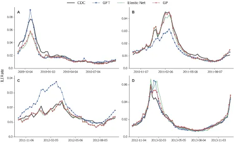
Query-only models. Table  1 enumerates the performance results for the three query-only models (GFT, Elastic Net and GP) and Fig. 1 presents the respective graphical comparison between predicted

GFT Elastic Net GP

Period Weeks r MAE×102 _{MAPE(%) r MAE×10}2 _{MAPE(%) r MAE×10}2 _MAPE(%)

2008–09 48 0.66 0.490 30.8 0.94 0.180 10.6 0.94 0.175 10.6

2009–10 57 0.97 0.324 14.4 0.99 0.499 15.1 0.99 0.451 14.6

2010–11 52 0.97 0.390 18.0 0.99 0.168 11.3 0.99 0.130 9.5

2011–12 52 0.92 0.550 33.1 0.94 0.131 9.8 0.94 0.129 9.8

2012–13 65 0.96 0.209 9.5 0.98 0.286 12.1 0.99 0.199 9.4

2008–13 274 0.89 0.381 20.4 0.92 0.260 11.9 0.95 0.221 10.8

www.nature.com/scientificreports/

and actual ILI rates (Supplementary Fig. S2 shows the results for 2008–09). Further details, such as the number of selected or nonzero weighted queries per case and model are shown in Supplementary Table S2. Evidently, the GP model outperforms both GFT and Elastic Net models. Using an aggregation of all inferences and the MAPE loss function, we see that Elastic Net yields an absolute performance improve-ment of 8.5% (relative improveimprove-ment of 41.7%) in comparison to GFT. The GP model in comparison to Elastic Net improves predictions further by 1.1% (relative improvement of 9.2%). We also observe that both Elastic Net and GP models cannot capture the ILI rate during the peak of the flu season for 2009– 10, whereas the GFT model over-predicts it. This could be a consequence of the the fact that 2009–10 was a unique flu period, as it is the only set of points expressing a pandemic in our data (H1N1 swine flu pandemic).

By measuring the influence of individual queries or clusters in each nowcast, we conduct a qualitative evaluation of the models, aiming to interpret some prediction errors. Our influence metric computes the contribution of a query or a cluster of queries by comparing a normal prediction outcome with an output had this query or cluster been absent from the input data (see SI, Estimation of query and cluster influ-ence in nowcasts). The GFT model is very unstable across the different flu seasons, sometimes exhibiting the smallest error (season 2009–10), and other times severely mispredicting ILI rates (seasons 2008–09, 2010–11 and 2011–12). Through an examination of a 21-week period (04/12/2011 to 28/04/2012), where major over-predictions occur (see Fig. 1C), and the estimation of the percentage of influence for each query in the weekly predictions, we deduced that queries unrelated to influenza were responsible for major portions of the final prediction. The query ‘rsv’ (where RSV stands for Respiratory Syncytial Virus) accounts on average for 24.5% of the signal, overtaking the only clearly flu-related query with a signif-icant representation (‘flu symptoms’ expressing 17.5% of the signal); the top five most influential que-ries also include ‘benzonatate’ (6.2%), ‘symptoms of pneumonia’ (6%) and ‘upper respiratory infection’ (3.9%), all of which are either not related to or may have an ambiguous contribution to ILI. Hence, the predictions were primarily influenced by content related to other types of diseases or generic concern, something that resulted in an over-prediction of ILI rates. For the same 21-week period, we performed a similar analysis on the features from the significantly better performing Elastic Net model. Firstly, the influence of each query is less concentrated, something expected given the increased number of nonzero weighted queries forming up the model (316 queries in Elastic Net vs. 66 in GFT). The features with the largest contribution were ‘ear thermometer’ (3.1%), ‘musinex’ (2.4%)—a misspelling of the ‘mucinex’ medicine, ‘how to break a fever’ (2.2%), ‘flu like symptoms’ (2.1%) and ‘fever reducer’ (2%), all of which may have direct or indirect connections to ILI. Note that none of the top five GFT features received a nonzero weight by Elastic Net, hinting that the latter model provided a probably better feature selection in this specific case.

During the last testing period (2012–13), we observe that the Elastic Net model marginally over-predicts the peak ILI rate, and sustains the same behavior in the 7 weeks that follow (Fig. 1D, weeks from 23-12-2012 to 16-02-2013). In the same 8-week period, the GP model manages to reduce Elastic Net’s MAPE from 31.9% to 14.9% (53% reduction of error). Elastic Net’s top influential queries for that time interval include irrelevant entries. Some examples, together with their average influence percentage and ranking, are ‘muscle building supplements’ (1.7%, 4th), ‘cold feet’ (1.3%, 10th), ‘what is carbon monoxide’ (1.2%, 13th) and ‘chemical formula for sugar’ (0.9%, 20th). The most influential query is ‘fever reducer’ (2.4%), a wording focused on a symptom of flu, but also of other diseases. We now determine the influence of each query cluster in the final GP prediction. Interestingly, the preceding queries, which may be unrelated to ILI (including ‘fever reducer’), are members of clusters with a very small average influence (from < .01% to a maximum of 1.3%). Notably, the most influential cluster includes queries about the ‘nba injury report’ (62.3%), whereas the second is clearly about flu (31.5%; ‘flu symptoms’, ‘flu prevention’ and ‘flu or cold’ were the most central terms). Initially, the model’s former choice may seem peculiar, however, the time series of ‘nba injury report’ reveal that this query is a great indicator of the winter season (see Supplementary Fig. S7). Nevertheless, k-means has separated this cluster from the disease-oriented ones.

In order to understand the nature and influence of the clustering in the GP models we draw our focus on the first testing period (2008–09; see Supplementary Fig. S2). There, the cluster with the strongest influence in the predictions (85.8% on average) is formed by queries that are very closely related to flu. The top five ones in terms of cluster centrality are the misspelled ‘flu symptons’, followed by ‘flu outbreak’, ‘how to treat the flu’, ‘flu season’ and ‘flu vs cold’. The second cluster has a significantly smaller influence (3.3%) and contains generic queries that seek information about various health conditions; the most central queries are ‘causes of down syndrome’, ‘trench foot’, ‘what causes pneumonia’, ‘what is a geno-type’ and ‘marfan syndrome pictures’. Looking at the remaining clusters, all of which have a moderate degree of influence, we see that their contents reflect different types of diseases or seasonal patterns. In particular, the top-3 most central queries in the third (2.6%), fourth (2.4%) and fifth (1.6%) clusters in terms of predictive influence are respectively {‘croup in infants’, ‘wooping cough’, ‘pnemonia symptoms’}, {‘best decongestant’, ‘dogs eating chocolate’, ‘how to stop vomiting’} and {‘dr king’, ‘rsv in adults’, ‘charles drew’}. Finally, there exists one more cluster that covers the topic of flu, but has a minor influence (1.3%). Notably, the queries of that cluster are less likely to have been issued by people with ILI as they are look-ing for more generic information about the disease, e.g., ‘flu duration’, ‘influenza b’, ‘cdc flu map’, ‘type a influenza’ and ‘tamiflu side effects’ are the most central queries.

Query models in an AR process. Nowcasts from the GFT, Elastic Net and GP models are used as a one-dimensional exogenous input in the ARMAX model defined by Eq. (6). We also include an AR baseline prediction, where only CDC data are used. During training, we compare multiple orders (val-ues for p and q) and select a model based on Akaike Information Criterion39_{. AR model training starts} from season 2008–09 (to be able to include out-of-sample query only predictions), and the first period of testing is 2009–10. Table 2 enumerates the performance results of the applied ARMAX models, using CDC ILI data with a time lag of 1 or 2 weeks from the current prediction. The best performance is achieved when GP nowcasts are used in the ARMAX framework (AR + GP), with a cumulative MAPE equal to 5.7% or 7.3% when a 1- or 2-week lag is applied respectively. Focusing on the 2-week lag as it reflects the delay of the actual CDC ILI reporting, the AR + GP model yields a 5.2% improvement over AR + Elastic Net, 28.4% over AR + GFT and 49% over the AR ILI baseline. Figure 2 plots the AR + GP

AR AR+GFT AR+Elastic Net AR+GP Period(Lag) r MAE MAPE r MAE MAPE r MAE MAPE r MAE MAPE

2009–10 (1) 0.98 0.314 11.2 0.99 0.173 7.4 ≈ 1 0.110 5.1 ≈ 1 0.123 5.9

2010–11 (1) 0.98 0.163 8.6 0.98 0.150 7.9 0.99 0.085 5.3 0.99 0.084 5.2

2011–12 (1) 0.95 0.092 6.4 0.95 0.098 6.8 0.95 0.099 6.9 0.95 0.101 7.0

2012–13 (1) 0.97 0.170 6.7 0.98 0.148 6.2 0.99 0.135 6.6 0.99 0.108 5.0

2009–13 (1) 0.97 0.187 8.2 0.98 0.143 7.0 0.99 0.109 6.0 0.99 0.105 5.7

2009–10 (2) 0.92 0.605 21.4 0.97 0.274 10.7 0.99 0.146 6.6 0.99 0.163 7.6

2010–11 (2) 0.92 0.305 15.6 0.95 0.250 12.5 0.99 0.110 6.7 0.99 0.102 6.3

2011–12 (2) 0.88 0.141 9.9 0.88 0.143 9.8 0.93 0.120 8.4 0.93 0.124 8.6

2012–13 (2) 0.92 0.280 10.6 0.95 0.206 8.3 0.98 0.187 8.7 0.98 0.146 7.0

2009–13 (2) 0.87 0.336 14.3 0.96 0.219 10.2 0.99 0.144 7.7 0.99 0.135 7.3

Table 2. Nowcasting performance (r, MAE × 102_{, MAPE(%)) of autoregressive ILI estimators}

www.nature.com/scientificreports/

nowcasts against the baseline AR and the ground truth ILI rates, when a 2-week lag is assumed. Apart from the significant prediction accuracy that the AR + GP model provides, we also observe that the incorporation of query information dramatically reduces the uncertainty of the predictions under all testing periods. Figure 3 draws an additional comparison, where the query-only model (GP) is plotted against its AR version. Interestingly, for the testing period 2009–10, it becomes evident that the AR + GP model is now capturing the peak of the flu season. Furthermore, the prediction intervals become tighter, especially when ILI rates are high (see Fig. 3D). It is important, however, to note that the uncertainty in the query-only prediction is not propagated through to prediction; the AR + GP procedure sees the GP regression as a form of data preprocessing.

We found that predictive errors in query-only models display auto-correlated structure that can be exploited for improved prediction (see Supplementary Fig. S6). The contribution of the ARMAX frame-work is that it can directly model this, effectively resetting the mean value of the prediction to a more likely location. An examination of the predictive period and the Q—Q plot of normalized logit-space errors (see Supplementary Fig. S5), shows a systematic bias in query-only experiments that is mitigated by the addition of the AR components. The improvement of the AR + GP and AR + Elastic Net models over the AR + GFT can be attributed to the higher query-only correlation with the CDC ILI signal, and the AR component’s ability to incorporate information about the natural autocorrelation in the signal.

A more fine-grained analysis of the predictions, when they really matter, i.e., during the peaking moments of a flu season, provides additional support for the improvements brought by the new query modeling methodology. Including weeks that belong to the .85 quantile of the seasonal CDC ILI rates (7 to 10 weeks per season), we measure the nowcasting performance of all the investigated models; the results are enumerated in Table 3. There, we observe that the GP model exhibits a similar MAPE to its general average performance, whereas the other models are much more error prone. For example, in the query-only results, Elastic Net’s cumulative MAPE during peak flu periods increases to 15.8% (from 11.9% overall), whereas GP’s error rate remains at the same levels (11% from 10.8%).

Discussion

We have presented an extensive analysis on the task of nowcasting CDC ILI rates based on queries submitted to an Internet search engine. Previously proposed (GFT) or well established (Elastic Net) methods have been rigorously assessed, and a new nonlinear approach driven by GPs has been proposed. In addition, query-only models were complemented by autoregressive components, merging traditional

syndromic surveillance outputs with inferences based on user-generated content. Overall the nonlinear GP approach, either in a query-only or an autoregressive format, performed better than the investigated alternatives. By conducting a qualitative analysis, we attempted to understand the shortcomings or the benefits of these regression models. A clear disadvantage of the original GFT model13 _{was the merging} of all query data into a single variable; in several occasions, this aggregation was injecting non directly flu-related queries (referring to a different disease or expressing a generic concern) that significantly affected the final prediction. Such queries may have been removed through manual inspection, making the whole system semi-automatic, but nevertheless this would not have resolved the overfitting caused by the limited expressiveness of the learning algorithm.

It is important to note that the presented AR + GP model achieves state-of-the-art performance compared to related recent works in the literature. In particular, the AR model proposed by Paul and Dredze37 _{that combines Twitter-based estimates}16,40 _{with prior CDC ILI rates, reaches a MAE (× 10}2_{) of} .190 when a 1-week lagged ILI rate is incorporated. Experiments in this paper were conducted for the years 2011–14; our AR + GP model (with a 1-week lag) yields a cumulative MAE of .098 during 2011–13, whereas the MAE of the GP query-only model is .156. Similarly, our model outperforms AR setups built

Figure 3. Comparison of nowcasts between the autoregressive model AR + GP and the query-only GP model together with their corresponding uncertainty intervals. (A–D): Flu seasons 2009–10, 2010–11, 2011–12 and 2012–13 respectively.

MAPE

Period #of weeks θ GFT ElasticNet GP AR + GFT AR + ElasticNet AR + GP

2008–09 7 2.47% 17.3 4.3 3.7 — — —

2009–10 9 4.21% 7.8 29.9 24.7 10.9 5.7 6.3

2010–11 8 3.11% 30.7 6.9 4.3 15.4 6.5 6.0

2011–12 8 1.93% 55.2 8.4 7.2 9.4 7.6 7.3

2012–13 10 3.26% 16.1 24.0 12.3 15.7 12.7 9.9

2008(9)–13 42 (35) NA 24.8 15.8 11.0 13.0 8.3 7.5

www.nature.com/scientificreports/

specifically on top of the publicly available GFT outputs, namely from Preis and Moat36_{, with a MAE of} .133 (during 2010–13), and from Lazer et al.20_{, with a MAE of .232 (during 2011–12).}

Confirming the estimations of related work7,20_{, the previous GFT query-only method did not have} a stronger predictive power than a 2-week delayed AR model based on CDC reports (20.4% vs. 14.3% MAPE, respectively). However, by allowing a greater expressiveness and by performing regularized regression some of the modeling issues were resolved. In fact, the query-only model based on Elastic Net regularization delivered a much better performance (11.9% MAPE), which improved with the GP model (10.8% MAPE). The operation on clusters of related queries makes the proposed GP model more robust to sudden changes in the frequency of single queries, that may happen due to media hype or other data corruption scenarios (e.g., ‘fake’ query attacks).

Looking further into the AR modeling and judging via the empirical predictive performance, we deduce that CDC data can be a useful addition when their lag is up to 4 or 5 weeks (see Supplementary Table S5). After this point, the AR + GP model does not benefit from the addition of ILI information, i.e., its performance falls back to the levels of query-only modeling. However, without query information, the equivalent AR CDC-based projections from a 3-week lag and onwards are becoming quite unreliable. This highlights some additional potential use cases of search query based surveillance, for example, in situations where a health surveillance system is blocked for a period greater than 2 weeks or ILI estimates are released on a monthly basis.

An interesting conclusion which came of as an intermediate result of our analysis was the observation that basic natural language processing techniques, such as stemming, stop-word removal or the extrac-tion of n-grams from the search query text, did not improve performance (see Supplementary Table S1). This can potentially highlight the quality of the signal enclosed in the data, at least at a national level density, as text preprocessing worsens rather than enhances information.

We note that a generic limitation for this line of research is the non-existence of a solid ‘gold stand-ard’. Traditional health surveillance data is based on the subset of the population that uses healthcare services, and we are aware that on average non-adults or the elderly are responsible for the majority of doctor visits or hospital admissions41_{. Thus, the provided ILI rates may not always form a definite ground} truth. Those potential biases are carried onto the query-only models through the means of supervised learning, and their impact becomes stronger in the updates of an AR model. On a more technical level, the increased expressiveness of the nonlinear GP model also comes at a price of interpretability, making harder to isolate the contribution of a single query. However, we can still interrogate the hyperparameters of each query cluster and see which contributes most to the marginal variance of predictions.

As these findings are turned into a real-time system, some additional and equally important concepts need to be investigated, such the optimal length of the training window, i.e., how and when should the system forget past information in order to adapt better to newly formed concepts. Research on combin-ing the multiple user-generated resources that have emerged in the recent years needs to be attempted, hypothesizing that it may provide a greater penetration in the population and, consequently, an even better accuracy. Finally, extensions of this work should consider combining the presented core models with network-based, more epidemiology-centric findings, where interesting properties of an infectious disease, such as geography42 _{or the source of spreading}43,44_{, could be potentially captured.}

References

1. Cha, M., Kwak, H., Rodriguez, P., Ahn, Y.-Y. & Moon, S. I Tube, You Tube, Everybody Tubes: Analyzing the World’s Largest User Generated Content Video System. In Proc. of the 7th ACM SIGCOMM Conference on Internet Measurement, IMC ‘07, 1-14 (ACM, San Diego, California, USA 2007).

2. Kwak, H., Lee, C., Park, H. & Moon, S. What is Twitter, a Social Network or a News Media? In Proc. of the 19th International Conference on World Wide Web, WWW ‘10, 591–600 (ACM, Raleigh, North Carolina, USA 2010).

3. Choi, H. & Varian, H. R. Predicting the Present with Google Trends. Economic Record88, 2–9 (2012).

4. Tumasjan, A., Sprenger, T. O., Sandner, P. G. & Welpe, I. M. Predicting Elections with Twitter: What 140 Characters Reveal about Political Sentiment. In Proc. of 4th International AAAI Conference on Weblogs and Social Media, ICWSM ‘10, 178–185 (AAAI, Washington, DC, USA 2010).

5. O’Connor, B., Balasubramanyan, R., Routledge, B. R. & Smith, N. A. From Tweets to Polls: Linking Text Sentiment to Public Opinion Time Series. In Proc. of the 4th International AAAI Conference on Weblogs and Social Media, ICWSM ‘10, 122–129 (AAAI, Washington, DC, USA 2010).

6. Bollen, J., Mao, H. & Zeng, X. Twitter mood predicts the stock market. Journal of Computational Science2, 1–8 (2011). 7. Goel, S., Hofman, J. M., Lahaie, S., Pennock, D. M. & Watts, D. J. Predicting consumer behavior with Web search. PNAS107,

17486–17490 (2010).

8. Scott, S. L. & Varian, H. R. Predicting the Present with Bayesian Structural Time Series. Inter J Math Model Num Opt5, 4–23 (2014).

9. Polgreen, P. M., Chen, Y., Pennock, D. M., Nelson, F. D. & Weinstein, R. A. Using Internet Searches for Influenza Surveillance.

Clin Infect Dis47, 1443–1448 (2008).

10. Lampos, V. & Cristianini, N. Tracking the flu pandemic by monitoring the Social Web. In Proc. of the 2nd International Workshop on Cognitive Information Processing CIP ‘10, 411–416 (IEEE, Elba Island, Italy 2010).

11. Johnson, H. A. et al. Analysis of Web access logs for surveillance of influenza. Stud Health Technol Inform107, 1202–1206 (2004). 12. Eysenbach, G. Infodemiology and Infoveillance: Framework for an Emerging Set of Public Health Informatics Methods to

Analyze Search, Communication and Publication Behavior on the Internet. J Med Internet Res.11, e11 (2009). 13. Ginsberg, J. et al. Detecting influenza epidemics using search engine query data. Nature457, 1012–1014 (2009).

15. Lampos, V. & Cristianini, N. Nowcasting Events from the Social Web with Statistical Learning. ACM Trans Intell Syst Technol3,

72:1–72:22 (2012).

16. Lamb, A., Paul, M. J. & Dredze, M. Separating Fact from Fear: Tracking Flu Infections on Twitter. In Proc. of of the 2013 Conference of the North American Chapter of the Association for Computational Linguistics: Human Language Technologies, NAACL-HLT ‘13, 789–795 (ACL, Atlanta, Georgia, USA 2013).

17. Paul, M. J. & Dredze, M. Discovering Health Topics in Social Media Using Topic Models. PLoS ONE9, e103408 (2014). 18. Cook, S., Conrad, C., Fowlkes, A. L. & Mohebbi, M. H. Assessing Google Flu Trends Performance in the United States during

the 2009 Influenza Virus A (H1N1) Pandemic. PLoS ONE6, e23610 (2011).

19. Olson, D. R., Konty, K. J., Paladini, M., Viboud, C. & Simonsen, L. Reassessing Google Flu Trends Data for Detection of Seasonal and Pandemic Influenza: A Comparative Epidemiological Study at Three Geographic Scales. PLoS Comput Biol9, e1003256 (2013).

20. Lazer, D., Kennedy, R., King, G. & Vespignani, A. The Parable of Google Flu: Traps in Big Data Analysis. Science343, 1203–1205 (2014).

21. Dixon, M. & Wiener, G. TITAN: Thunderstorm identification, tracking, analysis, and nowcasting - A radar-based methodology.

J Atmos Oceanic Technol10, 785–797 (1993).

22. Giannone, D., Reichlin, L. & Small, D. Nowcasting: The real-time informational content of macroeconomic data. J Monet Econ 55, 665–676 (2008).

23. Culotta, A. Lightweight methods to estimate influenza rates and alcohol sales volume from Twitter messages. Lang Resour Eval 47, 217–238 (2013).

24. Hastie, T., Tibshirani, R. & Friedman, J. The Elements of Statistical Learning (Springer, 2009).

25. Tibshirani, R. Regression shrinkage and selection via the lasso. J Roy Stat Soc B Met58, 267–288 (1996). 26. Zhao, P. & Yu, B. On Model Selection Consistency of Lasso. J Mach Learn Res7, 2541–2563 (2006).

27. Zou, H. & Hastie, T. Regularization and variable selection via the elastic net. J Roy Stat Soc B Met67, 301–320 (2005). 28. Lampos, V., Aletras, N., Preotiuc-Pietro, D. & Cohn, T. Predicting and Characterising User Impact on Twitter. In Proc. of the

14th Conference of the European Chapter of the Association for Computational Linguistics, EACL ‘14, 405–413 (ACL, Gotheburg, Sweden 2014).

29. Cohn, T., Preotiuc-Pietro, D. & Lawrence, N. Gaussian Processes for Natural Language Processing. In Proc. of the 52nd Annual Meeting of the Association for Computational Linguistics: Tutorials ACL ‘14, 1–3 (ACL, Baltimore, Maryland, USA, 2014). 30. Rasmussen, C. E. & Williams, C. K. I. Gaussian Processes for Machine Learning (MIT Press, 2006).

31. Matérn, B. Spatial Variation (Springer, 1986).

32. Lloyd, S. Least squares quantization in PCM. IEEE Trans Inf Theory28, 129–137 (1982).

33. Arthur, D. & Vassilvitskii, S. K-means++ : The Advantages of Careful Seeding. In Proc. of the 18th Annual ACM-SIAM Symposium on Discrete Algorithms SODA ‘07, 1027–1035 (SIAM, New Orleans, Louisiana, USA, 2007).

34. Manning, C. D., Raghavan, P. & Schütze, H. Introduction to Information Retrieval (Cambridge University Press, 2008). 35. Santillana, M., Zhang, D. W., Althouse, B. M. & Ayers, J. W. What can digital disease detection learn from (an external revision

to) Google Flu Trends? Am J Prev Med.47, 341–347 (2014).

36. Preis, T. & Moat, H. S. Adaptive nowcasting of influenza outbreaks using Google searches. Roy Soc Open Sci1 (2014). 37. Paul, M. J., Dredze, M. & Broniatowski, D. Twitter Improves Influenza Forecasting. PLoS Currents Outbreaks1 (2014). 38. Hamilton, J. D. Time Series Analysis vol. 2 (Princeton University Press, 1994).

39. Hyndman, R. J. & Khandakar, Y. Automatic Time Series Forecasting: The forecast Package for R. J Stat Softw27, 1–22 (2008). 40. Broniatowski, D. A., Paul, M. J. & Dredze, M. National and Local Influenza Surveillance through Twitter: An Analysis of the

2012–2013 Influenza Epidemic. PLoS ONE8, e83672 (2013).

41. O’Hara, B. & Caswell, K. Health Status, Health Insurance, and Medical Services Utilization: 2010. Curr Pop Rep. 70–133 (2012). 42. Daihai, H. et al. Global Spatio-temporal Patterns of Influenza in the Post-pandemic Era. Sci Rep.5 (2015).

43. Kitsak, M. et al. Identification of influential spreaders in complex networks. Nature Phys.6, 888–893 (2010).

44. Pinto, P. C., Thiran, P. & Vetterli, M. Locating the Source of Diffusion in Large-Scale Networks. Phys Rev Lett109, 068702 (2012).

Acknowledgments

We are grateful to Hal R. Varian for his constructive comments on earlier versions of this script. We also thank Rajan Patel and Steven L. Scott for their useful feedback; Tom Zhang and Wiesner Vos for assisting in the formation of intermediate search query data sets; David Duvenaud for technical advice. V.L. would also like to acknowledge the support from the EPSRC (UK) grant EP/K031953/1.

Author Contributions

V.L., A.C.M., S.C. and C.S. conceived the general concept of this research; V.L. and A.C.M. designed the models and performed the experiments; V.L. and A.C.M. wrote the paper; S.C. and C.S. contributed in writing.

Additional Information

Supplementary information accompanies this paper at http://www.nature.com/srep Competing financial interests: The authors declare no competing financial interests.

How to cite this article: Lampos, V. et al. Advances in nowcasting influenza-like illness rates using search query logs. Sci. Rep.5, 12760; doi: 10.1038/srep12760 (2015).