RESEARCH ARTICLE
10.1002/2014JD021710Key Points:
• We compute effective forcings from aerosol-cloud-radiation interactions in GCMs
• Total aerosol forcing is 25% direct effect and 75% indirect effect • Indirect effect comes mostly from
enhanced cloud scattering
Correspondence to:
M. D. Zelinka, [email protected]
Citation:
Zelinka, M. D., T. Andrews, P. M. Forster, and K. E. Taylor (2014), Quantifying components of aerosol-cloud-radiation interactions in climate models,J. Geo-phys. Res. Atmos.,119, 7599–7615, doi:10.1002/2014JD021710.
Received 28 FEB 2014 Accepted 27 MAY 2014
Accepted article online 1 JUN 2014 Published online 26 JUN 2014
Quantifying components of aerosol-cloud-radiation
interactions in climate models
Mark D. Zelinka1, Timothy Andrews2, Piers M. Forster3, and Karl E. Taylor1
1Program for Climate Model Diagnosis and Intercomparison, Lawrence Livermore National Laboratory, Livermore, California, USA,2Met Office Hadley Center, Exeter, UK,3School of Earth and Environment, University of Leeds, Leeds, UK
Abstract
The interaction of anthropogenic aerosols with radiation and clouds is the largest source of uncertainty in the radiative forcing of the climate during the industrial period. Here we apply novel techniques to diagnose the contributors to the shortwave (SW) effective radiative forcing (ERF) from aerosol-radiation-interaction (ERFari) and from aerosol cloud interaction (ERFaci) in experiments performed in phase 5 of the Coupled Model Intercomparison Project. We find that the ensemble mean SW ERFari+aci of−1.40 ± 0.56 W m−2comes roughly 25% from ERFari (−0.35 ± 0.20 W m−2) and 75% from ERFaci (−1.04 ± 0.67 W m−2). ERFari is made up of−0.62 ± 0.30 W m−2due to aerosol scattering opposed by +0.26±0.12 W m−2due to aerosol absorption and is largest near emission sources. The ERFari from nonsulfate aerosols is +0.13±0.09 W m−2, consisting of−0.15 ± 0.11 W m−2of scattering and +0.29±0.15 W m−2of absorption. The change in clear-sky flux is a negatively biased measure of ERFari, as the presence of clouds reduces the magnitude and intermodel spread of ERFari by 40–50%. ERFaci, which is large both near and downwind of emission sources, is composed of−0.99 ± 0.54 W m−2from enhanced cloud scattering, with much smaller contributions from increased cloud amount and absorption. In models that allow aerosols to affect ice clouds, large increases in the optical depth of high clouds cause substantial longwave and shortwave radiative anomalies. Intermodel spread in ERFaci is dominated by differences in how aerosols increase cloud scattering, but even if all models agreed on this effect, over a fifth of the spread in ERFaci would remain due solely to differences in total cloud amount.1. Introduction
Changes in aerosol concentrations over the industrial era have a direct effect on climate by absorbing and scattering shortwave (SW) radiation and can have multiple and varied effects on cloud properties that sub-sequently affect both SW and longwave (LW) radiation. The effects of aerosols on clouds have traditionally been referred to as indirect effects (which include effects on cloud albedo and cloud lifetime) and semidirect effects (which refer to aerosol-induced changes in thermal structure of the atmosphere that change clouds). However, in reality these processes are not easily distinguished either in observations or models, making interpretation difficult. Partly as a result of this, Chapter 8 of the fifth assessment report of the Intergovern-mental Panel on Climate Change (IPCC AR5) [Myhre et al., 2013a] chose to consider the effective radiative forcing from aerosol-cloud interactions (ERFaci) as a single entity that is distinguished from the effective radiative forcing from aerosol-radiation interactions (ERFari) [Boucher et al., 2013;Myhre et al., 2013b].
In IPCC AR5, the total (LW + SW) effective radiative forcing due to aerosols (ERFari+aci) is estimated to be
−0.90 [−1.9 to−0.1] W m−2and the ERFari is estimated to be−0.45 [−0.95 to +0.05] W m−2[Myhre et al., 2013a]. (Brackets indicate the 5 to 95% confidence intervals.) The ERFaci reported in AR5 is the difference between ERFari+aci and ERFari, thus yielding a value of−0.45 [−1.20 to 0.00] W m−2. Because climate model-derived estimates of ERF are typically more negative than observationally based estimates [Shindell et al., 2013], the ERF values reported in AR5 were adjusted to be smaller based on expert judgement. The large uncertainty in these ERF values—which is the dominant contributor to the uncertainty in the radiative forcing of the climate system over the industrial period—warrants exploration of the contributors to ERFari and ERFaci in models and demands accurate methods for systematically quantifying them. Here we bring new diagnostics to bear on ERF estimates, with an eye toward identifying aspects on which models agree and disagree and understanding the sources of disagreement.
components of ERFari. As noted in AR5, attempts to estimate ERFari in cloudy sky remain elusive [Boucher et al., 2013]. Although less difficult to quantify in models than in observations, a systematic intercomparison of ERFari across CMIP5 models has not been performed nor has the role of clouds in affecting ERFari in CMIP5 been quantified. Here we calculate ERFari under both clear-sky and all-sky conditions and quantify the substantial influence of clouds on both the scattering and absorption components of ERFari, indepen-dent of aerosol-induced changes in cloud properties. Moreover, rather than computing ERFaci as a residual from the other terms as is done in AR5, we compute ERFaci directly and separate it into components due to changes in cloud amount, scattering, and absorption.
Below, we describe the model experiments used as well as our methods for diagnosing the ERF components in the models. We then show the spatial patterns of ERF components and discuss the global mean values in each model, distinguishing between forcing due to sulfate and nonsulfate aerosols. We quantify the role of clouds in modifying the direct aerosol forcing relative to clear-sky conditions, and the implications of this for diagnosing ERF using clear-sky fluxes. We then explore the nature of aerosol-cloud interactions, incorporating additional cloud diagnostics. Finally, we explore the sources of intermodel spread in ERFari and ERFaci.
2. Data and Methods
Our study makes use of three 30 year fixed sea surface temperature (SST) experiments [Taylor et al., 2012] performed in nine global climate models (GCMs) as part of the fifth phase of the Coupled Model Inter-comparison Project (CMIP5). In the control run, sstClim, a repeating annual cycle of climatological SSTs and sea ice derived from each model’s preindustrial control run is imposed, and aerosols are set to prein-dustrial (1860) levels. The perturbation experiments, sstClimAerosol and sstClimSulfate, are identical to sstClim, except with emissions of anthropogenic aerosols (or their precursors) from year 2000 of the histor-ical experiment added. In sstClimAerosol, emissions of all anthropogenic aerosols are included, whereas in sstClimSulfate, only sulfate aerosol emissions are included. We will hereafter refer to the sstClimAerosol and sstClimSulfate experiments as All-Aerosol and Sulfate-Only experiments. We also derive estimates of the ERF due to nonsulfate aerosols by subtracting the Sulfate-Only results from the All-Aerosol results. Anomalies are computed by differencing climatological annual cycles between the perturbation and control experiments.
By perturbing only aerosol concentrations and by prescribing SSTs, these experiments are ideal for diag-nosing the effective radiative forcing (ERF) due to aerosol-radiation interactions (ari) and aerosol-cloud interactions (aci). The ERF is computed as the difference in top of the atmosphere (TOA) flux between the perturbed and control runs. As explained in Chapter 8 of IPCC AR5, whereas all surface and tropospheric conditions are kept fixed in determining radiative forcing, effective radiative forcing calculations allow all physical variables to respond to perturbations while keeping only sea surface temperature and sea ice fixed [Myhre et al., 2013a]. Thus, it is analogous to the “quasi-forcing” ofRotstayn and Penner[2001] and the “radia-tive flux perturbation” ofLohmann et al.[2010]. Because aerosols primarily impact the shortwave portion of the spectrum, we focus in this study on the shortwave (SW) ERF.
when compared with the more accurate PRP technique, which requires model output unavailable for most CMIP5 models.
The APRP technique allows for a partitioning of the change in reflected shortwave radiation between sur-face and atmosphere, with further separation of the atmospheric component between cloud and noncloud constituents. Unlike changes in cloud radiative effect (CRE =Ctot(Rov−Rclr), whereCtotis the total cloud frac-tion andRclrandRovare the net (downwelling minus upwelling) fluxes at the top of the atmosphere under clear-sky and overcast portions of the scene, respectively), the cloud components of the SW budget diag-nosed using APRP are due solely to cloud changes rather than to a combination of cloud and noncloud changes. Noncloud atmospheric components of reflected or absorbed SW radiation do not refer to a hypo-thetical clear-sky calculation in which clouds are ignored but rather to the part of the all-sky SW budget that arises due to changes in noncloud atmospheric constituents. In general, this arises primarily from changes in ozone, aerosols, and water vapor. In the idealized experiments considered in this study, the noncloud component is assumed to be entirely due to aerosols. Hereafter, we will use IPCC AR5 rather than APRP par-lance and refer to the change in SW radiation due to the noncloud atmospheric component as the effective radiative forcing due to aerosol-radiation interaction (ERFari). Similarly, the change in SW radiation due to the cloud component—which can be separated among changes in cloud amount, scattering, and absorp-tion —is hereafter referred to as the effective radiative forcing due to aerosol-cloud interacabsorp-tion (ERFaci). The change in surface albedo in these experiments is analogous to the radiative forcing due to absorbing aerosol on snow and ice, which is not considered to be part of ERFari [Myhre et al., 2013a]. Thus, one can think of ERFari as due solely to aerosols that are suspended in the atmosphere.
We stress that ERFari as calculated above is under all-sky conditions and therefore represents the radiative impact of changes in aerosols in the presence of clouds when cloud properties are held fixed. It is not the change in clear-sky SW radiation. However, for comparison we also compute the radiative impact of changes in aerosols in the absence of clouds by performing a hypothetical cloud-free APRP calculation. The differ-ence between this clear-sky calculation and the standard one in which the actual cloud fraction is used gives an estimate of the degree to which the presence of clouds (not their change) modifies the direct forcing by aerosols. To be consistent with the cloud feedback literature, we will refer to the difference (all-sky minus clear-sky) in these ERFari estimates as the cloud masking effect. Positive masking values means that the presence of clouds lessens the negative (cooling) effect of aerosols on the planet or increases the positive (warming) effect of aerosols on the planet.
Two caveats involving our decomposition are worth noting at this point. First, aerosol-enhanced SW absorp-tion can cause a change in the thermal structure of the atmosphere that affects cloud properties. IPCC AR5 includes changes in cloud properties that arise from such semidirect effects as part of ERFari. These are con-sidered distinct from aerosol indirect effects on clouds via microphysics, which fall into the ERFaci category. In this study, we count all changes in cloud properties as part of ERFaci. Thus, it is possible that semidirect effects are aliased into our ERFaci, though this effect is likely small given the secondary role of absorbing aerosols in these experiments. Second, our study makes use of fixed SST experiments in which the land surface temperature is allowed to evolve; thus, a small local cooling will occur over land that could lead to circulation and cloud changes that are not solely due to aerosol-cloud-interactions. We expect this effect to be quite small.
The models analyzed in this study are CanESM2, CESM1-CAM5, CSIRO-Mk3-6-0, GFDL-CM3, HadGEM2-A, IPSL-CM5A-LR, MIROC5, MRI-CGCM3, and NorESM1-M. Though available in the CMIP5 archive, we do not analyze BCC-CSM1.1 because in this model aerosol effects on cloud optical properties and lifetimes are neglected [Rotstayn et al., 2013]. Unless otherwise noted, all ERF values reported below are for shortwave radiation only.
3. Validation of Method
To build confidence in the accuracy of our method of decomposing the SW ERF components, we compare our results to those derived using the more direct technique ofGhan[2013] for All-Aerosol experiments performed using CAM5. In Ghan’s method, ERFari is computed asΔ(F−Fclean)and ERFaci is computed as
Figure 1.SW effective radiative forcing due to (left) aerosol-radiation interactions and (right) aerosol-cloud interac-tions in the All-Aerosol run of CAM5 estimated using (top) the APRP technique ofTaylor et al.[2007] and (middle) the technique ofGhan[2013], along with (bottom) their difference. Note that the color bar ranges differ among the panels.
aerosols,Fclear,cleanis the flux calculated neglecting scattering and absorption by both clouds and aerosols, andΔrefers to the difference between the aerosol-perturbed and control climates.
Estimates of ERFari and ERFaci using both techniques are compared in Figure 1. Spatial patterns of both estimates of ERFari and ERFaci are very similar, but local differences in certain regions are large enough to cause differences in the global mean. APRP-derived ERFari is 0.10 W m−2too negative in the global mean, and this is compensated by an ERFaci that is not negative enough (though the relative error is less than 5%) so that the total ERFari+aci is the same as that obtained with the Ghan method. Regions of positive ERFari west of Africa and South America are underestimated using the APRP technique.
There are a number of possible reasons why the APRP-derived results disagree slightly with those of Ghan. The assumption that noncloud atmospheric constituents absorb and scatter the same proportion of the radiation stream in overcast and clear scenes may not be valid. The assumption that all “noncloud” changes in SW flux are due to changes in aerosols is likely not strictly true, since a portion may be due to changes in other constituents (e.g., water vapor). Although the assumption that atmospheric absorption occurs only on the incident solar beam’s first pass through the atmosphere may introduce errors, we find that modifying the APRP technique to allow atmospheric absorption of downwellingandupwelling (reflected) shortwave fluxes (following the method ofDonohoe and Battisti[2011]) does not improve agreement with Ghan’s results (not shown), suggesting that our underestimate is not related to this effect. Finally, compared to APRP, Ghan’s technique can more completely account for cloud masking of ERFari, especially in locations with substantial submonthly aerosol-cloud variations.
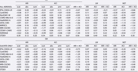
Table 1.Global and Annual Mean Effective Radiative Forcingsa
SW
ARI ACI LW NET
ALL AEROSOL scat abs sum scat abs amt sum ARI + ACI ARI ACI ARI + ACI ARI ACI ARI + ACI
IPSL-CM5A-LR −0.66 0.28 −0.38 −0.24 −0.01 0.15 −0.10 −0.47 0.01 −0.22 −0.21 −0.37 −0.31 −0.68
CanESM2 −0.58 0.17 −0.41 −0.51 0.01 −0.01 −0.50 −0.91 0.11 −0.04 0.07 −0.30 −0.54 −0.84
NorESM1-M −0.63 0.29 −0.34 −0.80 0.03 0.18 −0.59 −0.93 0.13 −0.17 −0.04 −0.21 −0.76 −0.97
CSIRO-Mk3-6-0 −1.13 0.49 −0.64 −0.76 0.08 0.00 −0.69 −1.33 −0.02 −0.21 −0.23 −0.66 −0.89 −1.55
HadGEM2-A −0.53 0.26 −0.27 −1.00 0.06 −0.13 −1.07 −1.34 0.14 −0.05 0.09 −0.13 −1.12 −1.24
GFDL-CM3 −0.91 0.41 −0.50 −0.99 −0.03 −0.13 −1.16 −1.66 0.11 0.02 0.13 −0.39 −1.14 −1.53
MIROC5 −0.66 0.16 −0.50 −0.93 −0.01 −0.28 −1.22 −1.73 0.22 0.27 0.49 −0.28 −0.96 −1.24
MRI-CGCM3 −0.11 0.12 0.01 −1.77 −0.09 −0.23 −2.09 −2.08 0.00 0.95 0.95 0.01 −1.14 −1.13
CESM1-CAM5 −0.33 0.21 −0.13 −1.93 0.06 −0.11 −1.98 −2.11 0.17 0.57 0.74 0.05 −1.41 −1.37
AVERAGE −0.62 0.26 −0.35 −0.99 0.01 −0.06 −1.04 −1.40 0.10 0.13 0.22 −0.25 −0.92 −1.17
STDEV 0.30 0.12 0.20 0.54 0.05 0.16 0.67 0.56 0.08 0.40 0.42 0.22 0.34 0.30
SW
ARI ACI LW NET
SULFATE ONLY scat abs sum scat abs amt sum ARI + ACI ARI ACI ARI + ACI ARI ACI ARI + ACI
IPSL-CM5A-LR −0.62 0.05 −0.57 −0.16 −0.02 0.00 −0.18 −0.75 0.07 −0.02 0.05 −0.50 −0.20 −0.70
CanESM2 −0.51 −0.05 −0.56 −0.46 0.00 −0.04 −0.50 −1.05 0.18 0.00 0.18 −0.38 −0.50 −0.88
CSIRO-Mk3-6-0 −0.82 −0.07 −0.89 −0.36 0.05 −0.09 −0.40 −1.29 0.17 0.03 0.20 −0.72 −0.37 −1.09
HadGEM2-A −0.26 −0.04 −0.30 −0.97 0.04 −0.13 −1.05 −1.35 0.10 0.09 0.19 −0.20 −0.96 −1.16
GFDL-CM3 −0.72 0.02 −0.70 −0.93 0.02 −0.14 −1.05 −1.75 0.16 0.03 0.19 −0.54 −1.02 −1.56
MIROC5 −0.51 −0.04 −0.56 −0.64 −0.02 −0.21 −0.87 −1.43 0.19 0.20 0.39 −0.37 −0.67 −1.03
MRI-CGCM3 −0.05 0.01 −0.04 −0.43 0.01 −0.05 −0.46 −0.50 −0.04 0.06 0.03 −0.08 −0.40 −0.48
AVERAGE −0.50 −0.02 −0.52 −0.56 0.01 −0.09 −0.64 −1.16 0.12 0.06 0.17 −0.40 −0.59 −0.98
STDEV 0.26 0.04 0.27 0.30 0.03 0.07 0.34 0.43 0.08 0.07 0.12 0.21 0.31 0.35
aAll estimates are given in units of W m−2. SW ERFari+aci is broken down into its components using the APRP technique. LW ERFaci is computed as the
change in LW cloud radiative effect, and LW ERFari is computed as LW ERFari+aci−LW ERFari.
across models (which is unknown), the strength of one model’s forcing relative to other models will be unchanged, and the contributors to intermodel spread can be accurately diagnosed. The advantages of the technique are that it does not require sophisticated model diagnostics or additional radiation calls, it can be applied systematically across models, and it allows for a partitioning of the SW forcing terms among many components.
4. Results
[image:5.612.38.579.590.727.2]ERF estimates, including the APRP-estimated decomposition of individual SW components, are provided in Table 1 for both the All-Aerosol and Sulfate-Only runs. ERF components due to nonsulfate aerosols, com-puted as the difference between All-Aerosol and Sulfate-Only values, are given in Table 2. Estimates of LW
Table 2.Global and Annual Mean Nonsulfate Aerosol Effective Radiative Forcingsa
SW
ARI ACI LW NET
NONSULFATE scat abs sum scat abs amt sum ARI + ACI ARI ACI ARI + ACI ARI ACI ARI + ACI
IPSL-CM5A-LR −0.04 0.23 0.19 −0.08 0.01 0.14 0.08 0.27 −0.06 −0.20 −0.26 0.13 −0.12 0.02
CanESM2 −0.07 0.22 0.15 −0.05 0.01 0.03 −0.01 0.14 −0.07 −0.04 −0.11 0.08 −0.05 0.03
CSIRO-Mk3-6-0 −0.31 0.56 0.25 −0.41 0.03 0.09 −0.29 −0.03 −0.19 −0.24 −0.43 0.06 −0.52 −0.46
HadGEM2-A −0.27 0.30 0.03 −0.03 0.01 0.00 −0.02 0.01 0.04 −0.14 −0.10 0.08 −0.16 −0.08
GFDL-CM3 −0.19 0.39 0.20 −0.07 −0.06 0.01 −0.11 0.08 −0.05 −0.01 −0.05 0.15 −0.12 0.03
MIROC5 −0.15 0.20 0.05 −0.29 0.01 −0.07 −0.36 −0.30 0.03 0.06 0.10 0.09 −0.29 −0.21
MRI-CGCM3 −0.05 0.11 0.05 −1.34 −0.11 −0.18 −1.63 −1.58 0.04 0.89 0.93 0.09 −0.74 −0.65
AVERAGE −0.15 0.29 0.13 −0.32 −0.01 0.00 −0.33 −0.20 −0.04 0.05 0.01 0.10 −0.29 −0.19
STDEV 0.11 0.15 0.09 0.47 0.05 0.11 0.59 0.63 0.08 0.39 0.44 0.03 0.26 0.27
Figure 2.(a) Ensemble mean SW effective radiative forcing in the All-Aerosol run and its separation into (b) aerosol-radiation interactions and (c) aerosol-cloud interactions. ERFari is further separated into its (d) scattering and (e) and absorption components, and ERFaci is further separated into its cloud (g) scattering, (h) absorption, and (i) amount components. The ERFari (mask) term shown in Figure 2f measures the effect of the presence of clouds on the ERFari, with positive values indicating that ERFari is less negative owing to the presence of clouds. The sum of Figures 2b and 2c equals Figure 2a. The sum of Figures 2d and 2e equals Figure 2b. The sum of Figures 2g–2i equals Figure2c.
ERFaci are computed as the change in LW CRE. Although the change in LW CRE is an imperfect measure of LW ERFaci due to cloud masking effects as described in section 4.4, we expect it to be less biased than its counterpart in the SW because the aerosol direct effect is much smaller in the LW. LW results are discussed only briefly in the paper and are included in the tables for completeness.
4.1. Spatial Distribution of Ensemble Mean ERF Components
Maps of SW effective radiative forcing components for the All-Aerosol run are shown in Figure 2. ERFari+aci is negative almost everywhere, indicating the widespread cooling effect of aerosol-radiation and aerosol-cloud interactions, but with considerable spatial heterogeneity. Whereas ERFari is large only near emissions sources and falls off to near-negligible levels downwind (Figure 2b), the ERFaci remains large throughout the downwind environment (Figure 2c). Notably, ERFaci is substantially larger than ERFari over the eastern ocean basins, highlighting the role of aerosol in serving as cloud condensation nuclei and increasing the cloud droplet number concentrations of stratocumulus clouds in the models.
ERFari is characterized by a large hemispheric asymmetry, as first noted byKiehl and Briegleb[1993], with a negative scattering component throughout much of the NH and a much smaller component in the SH (Figure 2d). ERFari due to absorption is large only near the emissions sources of absorbing aerosols (e.g., black carbon associated with biomass burning), most notably in Southeast Asia and Equatorial Africa (Figure 2e). The pattern of cloud masking, which causes the ERFari to be less negative than it would be under clear skies, reflects the mean distribution of cloudiness weighted by the pattern of ERFari (Figure 2f ). Thus, it tends to be greatest in the vicinity of or immediately downwind of emissions sources. Cloud masking will be discussed further below.
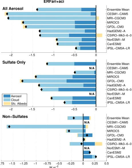
Figure 3.Global and annual mean APRP-derived SW ERFari+aci from the (top) All-Aerosol and (middle) Sulfate-Only runs. (bottom) Estimates of ERFari+aci due to nonsulfate aerosols present in the All-Aerosol run cal-culated by differencing the ERFs from the Aerosol and Sulfate-only runs. Components due to (dark blue) aerosol, (light blue) cloud, and (yellow) surface albedo are shown. Note that the total ERFari+aci, indicated by black diamonds, is the sum of aerosol and cloud components; the sur-face albedo component does not contribute to ERFari+aci but is shown for completeness. Models are sorted in order of their global mean values of SW ERFari+aci (black diamonds) in the All-Aerosol run. The aerosol compo-nent is equivalent to SW ERFari, while the cloud compocompo-nent is equivalent to SW ERFaci. Note that thexaxis range is different in Figure 3 bottom.
4.2. ERFari+aci
Figure 3 shows global mean estimates of ERFari+aci in each model and for the multimodel mean. Results are given for the All-Aerosol (top) and Sulfate-Only (middle) experiments, along with the difference between the two (bottom), which is the con-tribution from nonsulfate aerosols. In the ensemble mean, the All-Aerosol SW ERFari+aci of−1.40 W m−2comes 25% from ERFari (−0.35 W m−2) and 75% from ERFaci (−1.04 W m−2) (Table 1 and Figure 10), in qualitative agreement with the modeling results of bothLohmann et al.[2010] and Shindell et al.[2013]. In All-Aerosol, ERFaci is greater than ERFari in all but the IPSL-CM5A-LR model. However, in Sulfate-Only, three out of the six models (IPSL-CM5A-LR, CanESM2, and CSIRO-Mk3-6-0) have ERFari that exceeds ERFaci. It is noteworthy that CESM1-CAM5 and MRI-CGM3 have not only the largest ERFaci values of all models (possibly because they both allow aerosols to interact with ice clouds; see section 4.4) but also the smallest ERFari values of all mod-els. MRI-CGM3 is the only model with a positive (albeit tiny) direct effect.
Also shown in Figure 3 is the compo-nent of SW radiative forcing due to changes in surface albedo. A modest decrease in surface albedo is found in the CSIRO-Mk3-6-0 and MRI-CGCM3 models’ All-Aerosol runs, which have a large amount of deposition of absorbing aerosol on snow surfaces over the NH land masses and over the Arctic sea ice (not shown). In the other models, which do not include the deposition of black carbon on snow, there is a slight increase in surface albedo, owing to a small increase in snow cover induced by aerosol cooling over NH land masses.
Comparing All-Aerosol and Sulfate-Only experiments gives an estimate of the role of nonsulfate aerosols. We find that nonsulfate aerosols exert a systematically positive ERFari (due to absorption), a negative ERFaci in all models except in IPSL-CM5A-LR, and a positive ERFari+aci in all models except in CSIRO-Mk3-6-0, MIROC5, and MRI-CGCM3 (Figure 3 and Table 2).
4.3. ERFari
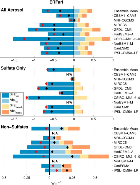
Figure 4.Effective radiative forcing due to aerosol-radiation interactions, separated into aerosol scattering (dark blue) and absorption (light blue) under clear skies, and the cloud masking of aerosol scattering (yellow) and aerosol absorption (orange). The sum of clear-sky terms is shown in red diamonds. Masking is defined as positive if the presence of clouds hides a negative forcing or enhances a positive forcing. The sum of all four terms is shown in black diamonds and is equivalent to the ERFari shown in dark blue bars in Figure 3. Note that thexaxis range is different in Figure 4 (bottom).
because scattering and absorption roughly scale with concentration for many nonsulfate aerosols. In the Sulfate-Only runs, the positive absorption component is negligible, as expected.
The yellow and orange bars in Figure 4 represent the influence of clouds on the scattering and absorption components of ERFari, respectively. We refer to these terms as cloud masking terms, and they are defined such that positive values indi-cate that the presence of clouds hides a negative forcing or enhances a positive forcing. The map of the mul-timodel mean total cloud masking is shown in Figure 2f, and the global mean values for each model are given in Table 3.
[image:8.612.234.519.578.717.2]Scattering of SW radiation by aerosols decreases in the presence of clouds compared to a cloud-free atmo-sphere, as indicated by the positive yellow Scatmaskbar in Figure 4. Phys-ically, this is due to two effects: First, the impact of aerosols will be reduced whenever they are shaded by over-lying clouds, since there will be less radiation to scatter. Second, aerosol scattering has a larger impact on the planetary albedo if the aerosol is located above a dark surface than if it is located above a highly reflec-tive cloud. In the ensemble mean, the presence of clouds acts to reduce by
Table 3.Clear-Sky Values and Cloud Masking of SW ERFari and the Bias inΔCRE With Respect to ERFacia
SW ERFariclr SW ERFarimask
ALL AEROSOL scat abs sum scat abs sum ΔSW CRE Bias
IPSL-CM5A-LR −0.85 0.16 −0.69 0.19 0.12 0.31 0.31
CanESM2 −0.76 0.10 −0.67 0.18 0.07 0.26 0.26
NorESM1-M −0.86 0.16 −0.71 0.23 0.13 0.37 0.40
CSIRO-Mk3-6-0 −1.56 0.29 −1.27 0.43 0.19 0.62 0.52
HadGEM2-A −0.66 0.15 −0.51 0.13 0.11 0.24 0.24
GFDL-CM3 −1.18 0.21 −0.96 0.26 0.20 0.46 0.50
MIROC5 −0.88 0.08 −0.80 0.22 0.08 0.30 0.31
MRI-CGCM3 −0.14 0.07 −0.07 0.03 0.05 0.08 0.03
CESM1-CAM5 −0.45 0.10 −0.35 0.12 0.11 0.22 0.23
AVERAGE −0.82 0.15 −0.67 0.20 0.12 0.32 0.31
STDEV 0.40 0.07 0.34 0.11 0.05 0.16 0.15
aAll estimates are given in units of W m−2. Please refer to Appendix A for the
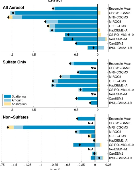
Figure 5.Effective radiative forcing due to aerosol-cloud interaction, separated into components due to changes in cloud scattering (dark blue), amount (light blue), and absorption (yellow). The sum of all three components (ERFaci) is shown in black diamonds, and is equivalent to the ERFaci shown in light blue bars in Figure 3. Note that thexaxis range is different in the bottom panel.
0.20 W m−2(0.16 W m−2in the Sulfate-Only run) the (negative) direct aerosol forcing from scattering effects (Table 3). In contrast, aerosol absorption of SW radiation in the All-Aerosol runs is systematically larger in the presence of clouds compared to a cloud-free atmo-sphere, as noted by the positive orange Absmaskbars. This effect is mainly due to the dependence of aerosol absorption on the underlying albedo. An absorbing aerosol will have a larger impact on the planetary albedo if it overlays a bright cloud than if it overlays a dark ocean. In the ensemble mean, the positive forcing from enhanced atmospheric absorption due to aerosols is roughly 40% smaller under clear-sky conditions (0.15 W m−2) than when clouds are present
(0.26 W m−2; Table 3). Thus, the presence of clouds acts to increase the (positive) direct aerosol forcing from absorption effects in the All-Aerosol run, increasing the heating within the atmosphere by 0.12 W m−2in the ensemble mean. This effect is negligible in the Sulfate-Only runs, since there is no aerosol absorption in the first place.
In sum, the presence of clouds (not their change) makes the negative ERFari sys-tematically smaller in magnitude than it would be in their absence (compare red and black diamonds) because of two reinforcing effects: clouds diminish the negative ERFari from aerosol scattering and enhance the positive ERFari from aerosol absorption. In the multimodel mean of the All-Aerosol runs, clouds reduce the mag-nitude of the negative multimodel mean ERFari by nearly 50% (from−0.67 to−0.35 W m−2) from what it would be under clear skies. In the Sulfate-Only runs, the masking effect is closer to 25% since sulfate aerosols are nonabsorbing and therefore cloud enhancement of absorption cannot contribute.
These masking terms mean that previously used simple approaches for estimating direct aerosol effects will be biased [see alsoGhan, 2013]. Specifically, the change in clear-sky flux is not the same as the ERFari, since the presence of clouds makes the effective radiative forcing from aerosols systematically less nega-tive. Although systematically negatively biased relative to the true direct effect, we find that the change in clear-sky flux is highly correlated with ERFari across models (r= 0.95 in All-Aerosol;r= 1.00 in Sulfate-Only), indicating that it serves as a useful proxy for quantifying intermodel spread in ERFari. However, intermodel spread in the change in clear-sky flux overestimates the “true” ERFari spread by about 60% in All-Aerosol and 40% in Sulfate-Only.
Figure 6.The percentage change in cloud optical depth for (top) high, (middle) midlevel, and (bottom) low clouds as computed from the ISCCP simulator for the All-Aerosol run. Locations in which cloud fraction is less than 2.5% in either the sstClim or sstClimAerosol runs are masked out.
Phase II results [Myhre et al., 2013b], perhaps because additional absorbing species are included among the nonsulfate aerosols or because of the inclusion of rapid adjustments in our ERF estimate. Our number is, on the other hand, smaller than the +0.40 W m−2black carbon radiative forcing reported in AR5 [Myhre et al., 2013a], though the latter is for the period 1750–2011 rather than 1860–2000. It is worth noting, however, that the absorbing effect of black carbon aerosols may be underestimated by up to a factor of 3 in current GCMs [Bond et al., 2013].
4.4. ERFaci
In Figure 5 we break down the ERFaci into components due to aerosol-induced changes in cloud scattering, amount, and absorption. The systematically negative scattering component is by far the dominant contrib-utor to ERFaci in every model. The cloud amount component is negative in all but the IPSL-CM5A-LR and NorESM1-M models’ All-Aerosol runs. The cloud scattering and amount components are quite well corre-lated across models (r= 0.60 in All-Aerosol,r= 0.72 in Sulfate-Only), though it is not obvious why this is the case.
All models considered here except IPSL-CM5A-LR and CanESM2 allow some effect of aerosols on precipi-tation formation, thereby allowing a cloud lifetime effect [Rotstayn et al., 2013]. Generally, the models with these parameterizations have cloud amount increases in the All-Aerosol and Sulfate-Only runs, and there-fore larger negative cloud amount components of ERFaci. It is noteworthy that ERFaci is least negative for the models without the cloud lifetime effect. The cloud absorption component of ERFaci is very small in every model and variable in sign across models. Both sulfate and nonsulfate aerosols enhance cloud albedo, making a systematically negative contribution to ERFaci.
Among all models considered, CESM1-CAM5, MRI-CGCM3, and MIROC5 have the largest values of ERFaci. This is mostly due to large negative cloud scattering components in these models, though MRI-CGCM3 and MIROC5 additionally have large negative amount components. MRI-CGCM3 and MIROC5 are also the only models in which nonsulfate aerosols cause an increase in cloud amount (CESM1-CAM5 cannot be assessed in this regard). Moreover, whereas estimates of LW ERFaci range from moderately negative to marginally positive among the other models, they are large and positive in CESM1-CAM5, MRI-CGCM3, and MIROC5 (Table 1). That these are the only models considered here that have parameterizations for the interaction of aerosols with ice clouds [Rotstayn et al., 2013] implies that aerosol influences on ice clouds may be driving these discernible differences and warrants further detailing of their aerosol-cloud interactions.
Figure 7.As in Figure 6 but for the absolute change in total cloud amount (in %) in each category.
Climatology Project (ISCCP) simulator [Klein and Jakob, 1999;Webb et al., 2001] for the four models in which these data were available. Whereas increases in cloud optical depth are most dramatic at low and midlevels in CanESM2 and HadGEM2-A, optical depth increases more for high clouds than for clouds at any other ver-tical level in both MIROC5 and MRI-CGCM3. These are also the only models in which global mean high cloud fraction increases in response to the aerosol perturbation (Figure 7).
The impacts on SW radiation of cloud changes at each of the three altitude ranges, computed using the ISCCP simulator cloud anomalies and cloud radiative kernels ofZelinka et al.[2012], are shown in Figure 8. Of the four models for which this calculation is possible, only in MIROC5 and MRI-CGCM3 are the contributions to ERFaci from high clouds substantial. In MRI-CGCM3, the contribution from high clouds is more than 3 times as large as the contribution from low clouds. In addition, MIROC5 and especially MRI-CGCM3 have
[image:11.612.62.550.482.706.2]Figure 9.Same as in Figure 6 but for cloud-induced LW radiation changes. Only the high cloud component is shown, as other components are negligible.
large positive LW ERFaci due to aerosol effects on high clouds (Figure 9). In contrast, the other two models have smaller, negative LW impacts from high cloud changes.
In summary, whereas high clouds in CanESM2 and HadGEM2-A become marginally brighter but less exten-sive and exert a positive SW ERFaci and negative LW ERFaci, those in MIROC5 and MRI-CGCM3 become substantially brighter and slightly more extensive and exert both a large negative SW ERFaci and a large pos-itive LW ERFaci. These results reflect the importance of aerosol interactions with ice-phase clouds on both LW and SW radiation.
As noted in section 4.3, the change in clear-sky SW radiation is a negatively biased measure of ERFari because clouds partially mask the direct aerosol effect. For similar reasons, the commonly used change in shortwave cloud radiative effect (CRE =Ctot(Rov−Rclr), whereRis defined as downwelling minus upwelling) as a measure of ERFaci will be systematicallypositivelybiased. As described inGhan[2013],ΔCRE is pos-itively biased with respect to the true aerosol indirect effect because the presence of absorbing aerosol above cloud increasesRovmore than it increasesRclrand the presence of scattering aerosol decreasesRclr more than it decreasesRov. In our decomposition, this positiveΔCRE bias is equivalent to the positive mask-ing effect of clouds on ERFari, plus the (generally small) cloud maskmask-ing of changes in surface albedo (see
Figure 10.The global and annual mean SW ERF values for the (top) All-Aerosol (9 models) and (bottom) Sulfate-Only (7 models) runs, sepa-rated into ERFari and ERFaci. ERFari, the dark blue “Aerosol” portion of the ARI + ACI bar, is separated into its (blue) scattering and (orange) absorp-tion components in the ARI bar. ERFaci, the light blue “Cloud” porabsorp-tion of the ARI + ACI bar, is separated into its (light blue) amount, (dark blue) scattering, and (orange) absorption components in the ACI bar. The sum of terms is indicated by the black diamond, with the intermodel standard deviation of each sum indicated by the horizontal error bar.
Appendix A). As noted above, we find that theΔCRE bias is system-atically positive (Table 3) and derive similar magnitude and patterns of biases asGhan[2013] finds for CAM5. The biases are greatest in the regions with largest ERFari, as expected. In the ensemble mean, theΔCRE biases are 0.31 W m−2for All-Aerosol and 0.16 W m−2for Sulfate-Only. The bias is systematically larger in the All-Aerosol runs due to the presence of absorbing aerosol. AlthoughΔCRE is a biased estimate, we find that it is well correlated with ERFaci across models (r= 0.99 in All-Aerosol;r= 0.96 in Sulfate-Only), indicating that it serves as a useful proxy for quan-tifying intermodel spread in ERFaci. Moreover, intermodel spread inΔCRE only slightly overestimates the “true” spread in ERFaci (by about 12% in All-Aerosol and 5% in Sulfate-Only).
4.5. Global and Ensemble Mean and Spread in ERF Terms
[image:12.612.176.414.395.647.2]compensation of the 0.62 W m−2cooling from aerosol scattering by the 0.26 W m−2warming from aerosol absorption (see also Table 1). Note that this value is in close agreement with both the direct aerosol radiative forcing from the MACC reanalysis of−0.40 W m−2[Bellouin et al., 2013] and the direct aerosol radiative effect estimate of−0.27 W m−2in the AeroCom Phase II simulations [Myhre et al., 2013b], even if one adds on an additional−0.10 W m−2to these estimates to account for rapid adjustments [Boucher et al., 2013].
The net (LW + SW) ERFaci of−0.92 W m−2reported here is roughly midway between the bottom-up (median value of−1.4 W m−2) and residual (−0.45 W m−2) estimates reported in AR5 (note that AR5 values are for 1750-2011). Unlike AR5, in which expert judgement values of ERFari and ERFaci are the same magnitude, we find that net ERFaci is nearly 4 times larger than net ERFari in the ensemble mean. In the Sulfate-Only runs, which have a negligible absorption component, ERFari and ERFaci are closer in magnitude in the ensemble mean.
4.6. Sources of Intermodel Spread in Effective Radiative Forcing 4.6.1. Spread in ERFari+aci
The substantial intermodel spread in ERFari+aci is dominated by the ERFaci component, whose spread (standard deviation of 0.67 W m−2) is over 3 times greater than that of ERFari (standard deviation of 0.20 W m−2; error bars in Figure 3, Table 1).
4.6.2. Spread in ERFari
The spread in ERFari reported in Table 1 is 35% larger in the Sulfate-Only runs (0.27 W m−2) than in the All-Aerosol runs (0.20 W m−2). This is true despite the fact that the spread in ERFari due to both scatter-ing and absorption is larger in the All-Aerosol runs. This result arises because models with larger negative ERFari due to scattering are also those with larger positive ERFari due to absorption in the All-Aerosol runs (r=−0.87). Thus, there is smaller uncertainty in the total ERFari than in its individual components, in agree-ment with the AeroCom Phase II results [Myhre et al., 2013b]. No such compensating effect exists in the Sulfate-Only runs since absorption is negligible.
Intermodel spread in ERFari is driven by both the scattering and absorption components. Intermodel spread in the scattering component of the direct aerosol forcing (0.30 W m−2) is 2.5 times as large as that due to the absorption component (0.12 W m−2). In the absence of clouds, it would be nearly 6 times as large (Tables 1 and 3). The presence of clouds acts to reduce (by 25%) the intermodel spread in direct aerosol forcing due to scattering while increasing (by 70%) the much smaller intermodel spread in direct aerosol forcing due to absorption. In sum, the presence of clouds reduces the intermodel spread in ERFari by nearly 40% (from 0.34 to 0.20 W m−2) from what it would be under clear skies.
4.6.3. Spread in ERFaci
The spread in ERFaci comes primarily from intermodel differences in aerosol effects on cloud scattering, especially in the Sulfate-Only runs, though intermodel differences in the cloud amount component are not negligible. The spread in the scattering component of ERFaci (0.54 W m−2) is 3.4 times larger than that in the amount component (0.16 W m−2).
Some of the intermodel spread in ERFaci is due to differences in how models parameterize their aerosol-cloud interactions, and some spread is due to differences in mean state cloud properties. Here we attempt to quantify these two sources of spread for the cloud scattering and amount components of ERFaci. Each component of ERFaci can be expressed as the product of a mean state cloud property,M, and a cloud property perturbation,P. Then, the spread in ERFaci due to intermodel differences inMholdingPat its ensemble mean value can be compared to spread in ERFaci due to intermodel differences inPholdingMat its ensemble mean value. Further details of the method are described in Appendix B.
Figure 11.Intermodel standard deviation in the SW ERFaci amount and scattering terms, broken down into contribu-tions from intermodel differences in mean state cloud properties and differences in cloud responses.
models had no differences in their mean state cloud properties, the intermodel spread in the ERFaci would remain nearly unchanged or even increase slightly.
However, it is interesting to note that, even if there were no intermodel disagreement in the response of cloud scattering to aerosols, over 20% of the intermodel spread in the cloud scattering component of ERFaci (0.12 out of 0.54 W m−2) would still remain due solely to intermodel differences in mean state total cloud fraction (Figure 11, bottom bar). In summary, the intermodel spread in aerosol indirect effects is dominated by intermodel differences in how clouds respond to aerosols, but even if models all agreed on this effect, there would remain appreciable intermodel spread due to variations in mean state cloud properties. These results are largely insensitive to whether we first normalize each models ERFaci by its ERFari to remove the influence of intermodel differences in aerosol loading.
We caution that this decomposition may underestimate the importance of mean state cloud properties in driving the response to aerosols, and its intermodel spread. This is because it neglects the fact that the change in cloud scattering, and to a lesser extent, the change in total cloud fraction, are themselves depen-dent on the mean state cloud properties. The albedo of clouds that are too optically thick in the control climate will be less sensitive to perturbations in optical depth arising from increased aerosol concentrations than optically thinner clouds [Twomey, 1991]. Likewise, total cloud fraction is bounded by zero and one, so increases in cloud fraction may be limited in regions of extensive cloud cover. Due to the lack of adequate cloud diagnostics we cannot pursue this line of investigation any further.
5. Conclusions
In this study we have applied a technique from the cloud feedback literature to quantify the individual com-ponents of the shortwave effective radiative forcing due to aerosol-radiation interactions and aerosol-cloud interactions in global climate model experiments that are forced by anthropogenic aerosols. The SW ERFari is separated into components due to aerosol scattering and absorption and is further decomposed into values that would occur under clear-skies as well as the degree to which the presence of clouds enhances or diminishes these clear-sky values. The SW ERFaci is separated into components due to changes in cloud amount, scattering, and absorption.
In the ensemble mean, the SW ERFari+aci of−1.40±0.56 W m−2comes 25% from ERFari (−0.35± 0.20 W m−2) and 75% from ERFaci (−1.04±0.67 W m−2). Negative ERFari from aerosol scattering is system-atically greater than positive ERFari from aerosol absorption; thus, the direct effect of aerosols on radiation is to cool the planet. Models with larger negative ERFari due to scattering tend to be those with larger pos-itive ERFari due to absorption (r=−0.87). Thus, there is smaller uncertainty in the total ERFari than in its individual components.
clear-sky conditions. This effect is smaller in the Sulfate-Only runs owing to the lack of aerosol absorption for clouds to enhance. An important implication of cloud masking effects is that commonly used simpler measures of ERFari (i.e., the change in clear-sky flux) are systematically negatively biased, and simpler mea-sures of ERFaci (i.e., the change in cloud radiative effect) are systematically positively biased. In both cases, however, the simpler measures are highly correlated with the “true” ERF values.
The large negative ERFaci, which exceeds the negative ERFari in all but one model analyzed, is primarily due to increases in cloud scattering. The cloud amount component is systematically smaller than the cloud scattering component, but the two are highly correlated across models. The importance of aerosols on ice clouds is made manifest in CESM1-CAM5, MRI-CGCM3, and MIROC5, which have the largest values of both SW and LW ERFaci among all models. In the latter two models (for which ISCCP simulator diagnostics are available), high clouds become substantially brighter and slightly more extensive and exert both a large negative SW ERFaci and a moderately positive LW ERFaci.
The substantial intermodel spread in ERFari+aci is dominated by the ERFaci component, whose spread is more than 3 times greater than that of ERFari. The intermodel spread in ERFaci is dominated by differences among models in how aerosols affect cloud albedo, with a smaller role for differences in how aerosols affect cloud amount. Even if all models agreed on the aerosol-induced enhancement of cloud albedo, however, over a fifth of the spread in the scattering component would remain simply due to mean state differences in cloud amount.
We have also estimated the effects of nonsulfate aerosols by comparing runs in which all anthropogenic aerosols are perturbed with those in which only sulfate aerosols are perturbed. We find that nonsulfate aerosols both scatter and absorb SW radiation, but the latter effect dominates, leading to an ERFari of 0.13±0.09 W m−2, consisting of 0.29±0.15 W m−2of absorption and−0.15±0.11 W m−2of scattering. Nonsulfate aerosols also (primarily) enhance cloud scattering, resulting in an ensemble mean ERFaci of
−0.33±0.59 W m−2. In most models the ERFari+aci from nonsulfate aerosols is small and positive, but in MIROC5 and MRI-CGCM3 it is large and negative, highlighting the role of nonsulfate aerosols in modifying ice cloud properties.
In closing, we note that fixed SST experiments like those used in this study are highly valuable in quantify-ing effective radiative forcquantify-ing and in understandquantify-ing rapid adjustments of clouds and other features of the climate to individual forcing agents. We encourage modeling centers to continue to perform these rela-tively inexpensive fixed SST experiments and to additionally consider other forcings like ozone, stratospheric water vapor, and solar irradiance [see alsoAndrews, 2014]. If absolute accuracy in the diagnosis of ERFari and ERFaci is necessary, it is best to employ the method ofGhan[2013], which requires output from an addi-tional “aerosol-free” radiation call. If small errors in the exact partitioning between ERFari and ERFaci can be tolerated, much insight can be gained (at least in the SW) simply from the standard two-dimensional diag-nostics requested in the CMIP protocol, as we have shown in this study. The details of cloud responses to individual forcings are even more clearly elucidated in models that have implemented the ISCCP simulator (c.f. Figures 5–8) [see alsoZelinka et al., 2013], and cloud responses in these models can be more readily com-pared with observations. Finally, the wide range of ERF values across models highlights the need to assess and evaluate the rapid adjustments and ERFs derived using GCMs with those derived using cloud-resolving models and large eddy simulations [e.g.,Johnson et al., 2004] and to reconcile these estimates with theory and observations.
Appendix A: Formal Breakdown of SW Radiative Budget Components
We separate the net (downwelling minus upwelling) SW radiation at the TOA into components accounting for the overcast (ov) and clear (clr) portions of a scene:
R= (1−Ctot)Rclr+Ctot(Rov). (A1)
assume that any change in noncloud atmospheric scattering and absorption is due entirely to aerosols. We can write the change inRas
ΔR= (1−Ctot)
[𝜕R
clr 𝜕𝛼clrΔ𝛼clr+
𝜕Rclr 𝜕𝛾aerΔ𝛾aer+
𝜕Rclr 𝜕𝜇aerΔ𝜇aer
]
+Ctot
[𝜕R
ov 𝜕𝛼ovΔ𝛼ov+
𝜕Rov 𝜕𝛾aerΔ𝛾aer+
𝜕Rov 𝜕𝜇aerΔ𝜇aer
]
+Ctot
[
𝜕Rov 𝜕𝛾cldΔ𝛾cld+
𝜕Rov 𝜕𝜇cldΔ𝜇cld
]
+ ΔCtot
[
Rov−Rclr
]
.
(A2)
The first bracketed term represents the impact of changes in surface albedo and aerosol scattering and absorption on the net SW radiation in the clear-sky portion of the scene, the second bracketed term rep-resents the impact of changes in surface albedo and aerosol scattering and absorption on the net SW radiation in the overcast portion of the scene, the third bracketed term represents the effect of changes in cloud scattering and absorption on the net SW radiation in the overcast portion of the scene, and the final term is the effect of changes in total cloud fraction on the net SW radiation of the scene.
ERFari is the sum of all terms that involve aerosol scattering (𝛾aer) and absorption (𝜇aer):
ERFari=Ctot
[
𝜕Rov 𝜕𝛾aerΔ𝛾aer+
𝜕Rov 𝜕𝜇aerΔ𝜇aer
]
+ (1−Ctot)
[
𝜕Rclr 𝜕𝛾aerΔ𝛾aer+
𝜕Rclr 𝜕𝜇aerΔ𝜇aer
]
. (A3)
The hypothetical ERFari computed assuming clear skies (Ctot=0) is
ERFariclr= 𝜕Rclr 𝜕𝛾aerΔ𝛾aer+
𝜕Rclr
𝜕𝜇aerΔ𝜇aer. (A4)
The cloud masking of ERFari is therefore
ERFarimask=ERFari−ERFariclr=Ctot
[𝜕(R
ov−Rclr) 𝜕𝛾aer Δ𝛾aer+
𝜕(Rov−Rclr) 𝜕𝜇aer Δ𝜇aer
]
. (A5)
The mask is equal to the sensitivity of radiation to aerosol scattering and absorption under clear skies subtracted from that under overcast skies, multiplied by total cloud fraction. Similarly, ERFaci is expressed as
ERFaci=Ctot
[𝜕R
ov 𝜕𝛾cldΔ𝛾cld+
𝜕Rov 𝜕𝜇cldΔ𝜇cld
]
+ ΔCtot
[
Rov−Rclr
]
, (A6)
where the terms are, respectively, the cloud scattering, absorption, and amount components. This can be compared with the change in cloud radiative effect:
ΔCRE= ΔR− ΔRclr. (A7)
The difference between the change in cloud radiative effect and ERFaci can, after some algebra, be expressed as
ΔCRE−ERFaci=ERFarimask+Ctot
[𝜕R
ov 𝜕𝛼ovΔ𝛼ov−
𝜕Rclr 𝜕𝛼clrΔ𝛼clr
]
. (A8)
Thus, the bias inΔCRE relative to the “true” ERFaci equals the cloud masking of ERFari plus an additional term representing the cloud masking of changes in surface albedo. The masking of changes in surface albedo is computed as the sensitivity of radiation to changes in surface albedo under clear skies subtracted from that under overcast skies, multiplied by total cloud fraction.
Appendix B: Quantifying Sources of Intermodel Spread in ERFaci
As shown in the equation (A6), ERFaci is the product of mean state cloud properties and perturbations to these cloud properties. For example, the ERFaci due to cloud scattering is
ERFaciscat=Ctot
[𝜕R
ov 𝜕𝛾cldΔ𝛾cld
]
and we can define the perturbed quantity,P, to be[𝜕Rov 𝜕𝛾cld
Δ𝛾cld]and mean state quantity,M, to beCtot. Now
for each model,i, we can representPandMin terms of a multimodel mean value (angled brackets) plus a deviation from the mean (prime symbol). The productPMcan then be expanded as follows:PiMi = ⟨P⟩⟨M⟩+⟨P⟩M′
i+P
′
i⟨M⟩+P
′
iM
′
i.Mdepends only on the mean state total cloud amount, whereasPdepends
on the response of cloud albedo to the aerosol perturbation.⟨P⟩M′is the product of the ensemble mean change in cloud scattering with the model-specificCtot; thus, spread in this component arises solely from intermodel spread in mean stateCtot. Similarly,P′⟨M⟩is the product of the model-specific change in cloud scattering with the ensemble meanCtot; thus, spread in this component arises solely from intermodel spread in the change in cloud scattering.P′M′is the covariance term. By definition, intermodel spread in⟨P⟩⟨M⟩is zero. We perform this same decomposition for the cloud amount component by settingPtoΔCtotandM to[Rov−Rclr].
References
Andrews, T. (2014), Using an AGCM to diagnose historical effective radiative forcing and mechanisms of recent decadal climate change,
J. Clim.,27(3), 1193–1209, doi:10.1175/JCLI-D-13-00336.1.
Bellouin, N., J. Quaas, J. J. Morcrette, and O. Boucher (2013), Estimates of aerosol radiative forcing from the MACC re-analysis,Atmos. Chem. Phys.,13(4), 2045–2062, doi:10.5194/acp-13-2045-2013.
Bond, T. C., et al. (2013), Bounding the role of black carbon in the climate system: A scientific assessment,J. Geophys. Res. Atmos.,118, 5380–5552, doi:10.1002/jgrd.50171.
Boucher, O., et al. (2013),Clouds and Aerosols, chap. 7, Cambridge Univ. Press, Cambridge, U. K., and New York.
Donohoe, A., and D. S. Battisti (2011), Atmospheric and surface contributions to planetary albedo,J. Clim.,24(16), 4402–4418, doi:10.1175/2011jcli3946.1, times Cited: 17 Battisti, David /A-3340-2013 Battisti, David /0000-0003-4871-1293 17.
Ghan, S. J. (2013), Technical note: Estimating aerosol effects on cloud radiative forcing,Atmos. Chem. Phys.,13(19), 9971–9974, doi:10.5194/acp-13-9971-2013.
Johnson, B. T., K. P. Shine, and P. M. Forster (2004), The semi-direct aerosol effect: Impact of absorbing aerosols on marine stratocumulus,
Q. J. R. Meteorol. Soc.,130(599), 1407–1422, doi:10.1256/qj.03.61.
Kiehl, J. T., and B. P. Briegleb (1993), The relative roles of sulfate aerosols and greenhouse gases in climate forcing,Science,260(5106), 311–314, doi:10.1126/science.260.5106.311.
Klein, S. A., and C. Jakob (1999), Validation and sensitivities of frontal clouds simulated by the ECMWF model,Mon. Weather Rev.,127, 2514–2531, doi:10.1175/1520-0493(1999)1272.0.CO;2.
Lohmann, U., L. Rotstayn, T. Storelvmo, A. Jones, S. Menon, J. Quaas, A. M. L. Ekman, D. Koch, and R. Ruedy (2010), Total aerosol effect: Radiative forcing or radiative flux perturbation?,Atmos. Chem. Phys.,10(7), 3235–3246.
Myhre, G., et al. (2013a),Anthropogenic and Natural Radiative Forcing, chap. 8, Cambridge Univ. Press, Cambridge, U. K., and New York. Myhre, G., et al. (2013b), Radiative forcing of the direct aerosol effect from AeroCom Phase II simulations,Atmos. Chem. Phys.,13(4),
1853–1877, doi:10.5194/acp-13-1853-2013.
Rotstayn, L., and J. Penner (2001), Indirect aerosol forcing, quasi forcing, and climate response,J. Clim.,14(13), 2960–2975, doi:10.1175/1520-0442(2001)014<2960:IAFQFA>2.0.CO;2.
Rotstayn, L. D., M. A. Collier, A. Chrastansky, S. J. Jeffrey, and J. J. Luo (2013), Projected effects of declining aerosols in RCP4.5: Unmasking global warming?,Atmos. Chem. Phys.,13(21), 10,883–10,905, doi:10.5194/acp-13-10883-2013.
Shindell, D., et al. (2013), Radiative forcing in the ACCMIP historical and future climate simulations,Atmos. Chem. Phys.,13(6), 2939–2974, doi:10.5194/acp-13-2939-2013.
Taylor, K. E., M. Crucifix, P. Braconnot, C. D. Hewitt, C. Doutriaux, A. J. Broccoli, J. F. B. Mitchell, and M. J. Webb (2007), Estimating shortwave radiative forcing and response in climate models,J. Clim.,20(11), 2530–2543, doi:10.1175/JCLI4143.1.
Taylor, K. E., R. J. Stouffer, and G. A. Meehl (2012), An overview of CMIP5 and the experiment design,Bull. Am. Meteorol. Soc.,93(4), 485–498, doi:10.1175/BAMS-D-11-00094.1.
Twomey, S. (1991), Aerosols, clouds and radiation,Atmos. Environ. Part A,25(11), 2435–2442, doi:10.1016/0960-1686(91)90159-5. Webb, M., C. Senior, S. Bony, and J. J. Morcrette (2001), Combining ERBE and ISCCP data to assess clouds in the Hadley Centre, ECMWF
and LMD atmospheric climate models,Clim. Dyn.,17, 905–922, doi:10.1007/s003820100157.
Zelinka, M. D., S. A. Klein, and D. L. Hartmann (2012), Computing and partitioning cloud feedbacks using cloud property histograms. Part I: Cloud radiative kernels,J. Clim.,25(11), 3715–3735, doi:10.1175/JCLI-D-11-00248.1.
Zelinka, M. D., S. A. Klein, K. E. Taylor, T. Andrews, M. J. Webb, J. M. Gregory, and P. M. Forster (2013), Contributions of different cloud types to feedbacks and rapid adjustments in CMIP5,J. Clim.,26(14), 5007–5027, doi:10.1175/jcli-d-12-00555.1.
Acknowledgments