Rochester Institute of Technology
RIT Scholar Works
Theses
Thesis/Dissertation Collections
5-12-2015
Allocation of Workers Utilizing Models with
Learning, Forgetting, and Various Work Structures
Austin T. Chacosky
Follow this and additional works at:
http://scholarworks.rit.edu/theses
This Thesis is brought to you for free and open access by the Thesis/Dissertation Collections at RIT Scholar Works. It has been accepted for inclusion in Theses by an authorized administrator of RIT Scholar Works. For more information, please [email protected].
Recommended Citation
Rochester Institute of Technology
Allocation of Workers Utilizing Models with Learning, Forgetting, and Various
Work Structures
A Thesis
Submitted in partial fulfillment of the requirements for the degree of
Master of Science in Industrial Engineering
in the
Department of Industrial & Systems Engineering Kate Gleason College of Engineering
by
Austin T Chacosky
DEPARTMENT OF INDUSTRIAL AND SYSTEMS ENGINEERING
KATE GLEASON COLLEGE OF ENGINEERING
ROCHESTER INSTITUTE OF TECHNOLOGY
ROCHESTER, NEW YORK
CERTIFICATE OF APPROVAL
M.S. DEGREE THESIS
The M.S. Degree Thesis of Austin Chacosky
has been examined and approved by the
thesis committee as satisfactory for the
thesis requirements for the
Master of Science degree
Approved by:
Dr. Scott E. Grasman, Thesis Advisor Date
AND
Dedication
This thesis is dedicated to my friends and family. Their accomplishments have continuously
Acknowledgements
This thesis would not have been possible without the support of many people. I offer many thanks
to my advisor, Dr. Scott Grasman, for reading my numerous revisions and for his guidance in
preparation of this research work. I would not have undertaken this work without the
encourage-ment and support of Dr. Mike Hewit to whom I am very grateful. I would also like to thank my
committee member, Dr. Michael Kuhl, for his guiding service and support. Additional thanks go to
Dr. Ruben Proano for sparking my interest in Operations Research and for sharing his computing
resources used for this work. Thanks to the Rochester Institute of Technology for providing me an
Allocation of Workers Utilizing Models with Learning, Forgetting,
and Various Work Structures
Abstract
Much of the literature on cross-training and worker assignment problems focus on simulating
pro-duction systems under cross-training methods. Many have found that for specific systems some
methods of allocating workers are better performing than others in terms of overall productivity and
ability to deal with change. This has lead researchers to create mathematical programming models
with a goal of finding optimal levels of cross-training by changing worker allocations. Learning and
forgetting curves have been a key method to improve the solutions produced by the optimization
models, but learning curves are often nonlinear causing increased solving times. Because of this,
most works have been restricted to modeling small, simple production systems.
This thesis studies the expansion of worker allocation models with human learning and
for-getting to include variable work structures, thus allowing the models to be used to address a larger
set of problems than previously possible. A worker assignment model with flexible inventory
con-straints capable of representing different production structures is constructed to demonstrate the
expansion. Utilizing a reformulation technique to counteract the increased solve times of learning
curve incorporation, the scale of the production systems modeled in this work is larger than in
similar works and closer to the scale of systems seen in industry. Production systems with multiple
products and corresponding due dates are modeled to better represent the production environment
in industry. Investigative tests including a 24 factorial experiment are included to understand the
performance of the model. The output of the optimization model is a schedule of worker
assign-ments for the planning horizon over all of the tasks in the modeled system. Production managers
could apply the schedule to their existing lines or run what-if scenarios on line structure to better
understand how alternative structures may affect worker training and line productivity over the
Contents
1 Introduction 7
2 Literature Review 10
3 Mathematical Programming Formulation of Worker Allocation Models with
Learning and Forgetting 19
3.1 Sets, Parameters, and Variables . . . 20
3.2 Worker Allocation Model with Learning and Forgetting . . . 21
3.3 Reformulation Technique . . . 24
3.3.1 Reformulation Variables & Parameters . . . 26
3.3.2 Reformulation Constraints . . . 27
3.4 Practicing Reduction . . . 28
4 Research Strategy 30 4.1 Model Responses . . . 30
4.2 Experimental Design Factors . . . 30
4.3 Generation of Factor Random Values . . . 34
4.4 Algorithm Tuning . . . 34
5 Results 36 5.1 Experiment 1 . . . 38
5.2 Experiment 2 . . . 52
6 Discussion 55
7 Conclusions and Future Work 56
8 Bibliography 60
1
Introduction
Faisal Hoque once wrote,“Constant change is the new dynamic of the global economy, making
agility more necessary than ever” [Hoque, 2009]. In production systems, change often means
vari-able workloads, new products, untrained workers, and new production structures. Dealing with
these changes is an ever important problem for production managers. A common solution is to
reallocate workers to where they are needed. Transferring labor between areas with a surplus of
workers and those with a deficit can provide relief when demands shift. The problem of deciding
which workers will cover which tasks grows quickly with the number of workers and tasks. Soon
the possible allocations become too large for production managers to evaluate and choose the
so-lution which best satisfies their objectives. Because of the often vast number of combinations of
workers and tasks, worker allocation problems are great applications of mathematical programming
optimization. The objective of such programs is commonly to minimize the gap between the need
for workers and supply of labor by allocating the workforce to where it is needed. When there
are many workers to reallocate and the impacts of those decisions are vast, using mathematical
modeling can make a world of difference.
Worker allocation models are not the complete answer though. Sometimes there are needs
that cannot be filled with the current workforce. Even when the capital and labor are available,
the problem can be training. Forethought and planning are often key to success in business.
Cross-training is one way that production managers can prepare for changes to their business.
Cross-training involves teaching workers to perform multiple tasks. This simple concept has many
benefits. First, when workers know more than one or two tasks they can be reallocated to fill in
when other workers are sick, are out on vacation, or when additional labor is needed elsewhere.
Workers have a better chance of filling gaps. Second, cross-trained workers are mentally stimulated
when asked to learn new tasks and get less bored. Workers are happy to be challenged. Without
cross-training, workers are specialized in specific tasks and can become discontent [Nembhard and
Osothsilp, 2004]. In the past, before labor reform, this was not uncommon [Smith, 1776].
The study of industrial productivity is not something new. In the first chapter of his famous
work, “On the Wealth of Nations”, published in 1776, Adam Smith explains the benefits of what
he calls the Division of Labor. Smith states that in a manufacturing setting when work is split
into equal parts and given in equal share to workers, the productivity of each worker and the
Book 1, Smith states that when workers specialize in certain tasks, they get very good at those
specific tasks and the systems, as a whole, can produce more products [Smith, 1776]. Productivity
was an important factor to businesses then, it also is today, so Smith’s writing is of value. In a
later chapter, Smith notes that specialization can lead to worker dissatisfaction with work due to a
separation of the laborer from the product and the daunting repetition of specialized work [Smith,
1776]. This led to the idea of job rotation and eventually cross-training.
Cross-training workers is now a heavily adopted idea in many fields, but it is not a trivial
endeavor. Cross-training can be hard to implement well. Managers often rely on researchers,
cre-ating models to simulate cross-training policies, to better understand how cross-training workers
will affect production. Those models often focus on parameters such as task tenure, worker
mul-tifunctionality, and cross-training level, and how they affect productivity [Nembhard and Shafer,
2008]. As cross-training methodologies in industry involve workers rotating through different tasks,
task tenure is a measure of how often workers change tasks. Interruptions from learning lead to
workers forgetting their training. The relationship between task tenure and forgetting will be
fur-ther discussed later. The term worker multifunctionality refers to the number of different jobs on
which a worker is trained. Finally, cross-training level refers to the number of workers that are
training on the same job. A complete cross-training program must include levels for task tenure,
worker multinationality, and cross-training level. A good cross-training program has levels for the
parameters which balance cross-training benefits with its costs [Hewitt et al., 2013].
While cross-training has been shown to be useful in increasing flexibility of production
sys-tems, cross-training also has non-obvious costs that can depend on the structure of the systems.
These costs include direct training costs associated with instruction and materials for training,
de-creased productivity during the training process, and the dede-creased productivity due to forgetting
when workers are removed from primary task. Yang [2007], Sayin and Karabati [2007],
Nemb-hard and Norman [2007], Bokhorst and Gaalman [2009], Molleman and Slomp [1999], NembNemb-hard
and Osothsilp [2004], Malhotra et al. [1993] have proposed that there exists an optimal level of
cross-training for production systems that balances worker flexibility and system productivity.
To model the costs of cross-training, works such as Sayin and Karabati [2007], Nembhard and
Norman [2007], Nembhard and Osothsilp [2004], Malhotra et al. [1993] have utilized experiential
learning curves. Because job rotation involves placing workers on tasks that are new to them, there
are some negative impacts to cross-training that relate to human learning. It takes workers some
better model the rate at which workers acquire skill, learning curves have recently been used in
cross-training models. Incorporating learning into worker allocation cross-training models can lead
to gains in model validity, but often greatly increase formulation complexity due to the non-linearity
of useful learning curves [Sayin and Karabati, 2007, Nembhard and Norman, 2007].
Worker allocation models with learning are not currently designed to represent all systems.
Decreased productivity during training and worker forgetting is increasingly difficult to include in
worker allocation models with high fidelity, but has been accomplished on a small scale by
incorpo-rating functions of experiential learning into models of systems with cross-training. Modeling the
learning of workers in systems with multileveled product structures, involving many workers and
numerous products have largely been left unstudied in the cross-training modeling scope because
of solving difficulties. Through the use of new reformulation methods, which transform the model
from a nonlinear mixed integer program into a linear mixed integer program, those systems now
can be explored to see if results and conclusions from works studying smaller systems can be used
to explain behaviors of larger production systems of differing structures.
Specifically, in Dual Resource Constrained (DRC) systems, where both employees and capital
equipment are constrained, at least some employees must be trained on more than one task to cover
the tasks. Because of this, the loss of productivity due to worker learning is an issue in DRC
job-shop systems. When a worker is learning to operate a machine in a DRC system, there is one less
machine for a trained operator to be productive on and the cross-trained employee is taken off of a
task where he could have been more productive. For an overview of DRC studies see Hottenstein
and Bowman [1998]. This work focuses on expanding existing worker allocation models that include
human learning and forgetting in order to make cross-training worker allocations in DRC systems
with various work structures. Discussed later, this thesis introduces a worker allocation model with
learning, forgetting, and a flexible work structure to model various systems which practitioners
2
Literature Review
Because of its many benefits, cross-training and worker allocation problems are well represented
in the literature. Works that include human learning are of a particular interest in this work, and
those, while seeming to grow in recent popularity, are seen in much fewer numbers. Previous
laboratory and empirical studies have identified some aspects of cross training that have been
shown to affect the effectiveness of worker flexibility on a system. The aspects relating to this
thesis are summarized in the following table:
Worker
Multifunctionality The number of tasks the worker is trained on. Task Redundancy The number of workers trained on the same job.
Cross-training Distribution
The distribution of Worker Multifunctionality and Task Redundancy across
workers.
Task Tenure The length of time which a worker trains on a task before rotating to another
task to train.
Task Similarity The effect that learning a task has on the a worker’s productivity on other
analogous tasks of similar form.
Learning Rate The rate at which workers acquire skill on tasks during training.
Forgetting Rate The rate at which workers dispossess skill on tasks when not training.
Staffing Level The ratio of workers to tasks.
Worker Attrition The permanent loss of workers.
Absenteeism The temporary loss of workers due to sickness or vacation.
Due Dates The planned production schedule and associated deadlines.
Multiple Products The number of various products the system produces.
Worker Similarity The level of homogeneity between worker parameters.
The following subsections discuss some of these aspects.
Worker Multifunctionality, Task Redundancy, and Cross-training Distribution
There has been recent research regarding the subject of creating effective worker assignments.
Much of that research has used the assumption of constant worker productivity levels (e.g.
Molle-man and Slomp [1999], Bokhorst and GaalMolle-man [2009], and Campbell [2010]). Many of those models
out-put performance indicators are affected by certain cross-training methods such as Skill-Chaining,
a method which workers have overlapping task responsibilities [Hopp and Oyen, 2004]. Molleman
and Slomp [1999] show the effects of worker absenteeism, task redundancy, and worker
multifunc-tionality on system performance metrics in a descriptive manor. They identify task redundancy
as an effective way of countering absenteeism under varying levels of worker multifunctionality.
Cross-training with heterogeneously productive workers is shown to have differing effects on DRC
systems from those seen in Single Resource Constrained (SRC) Systems [Bokhorst and Gaalman,
2009]. Yang [2007] identifies that certain levels of cross-training distribution across the workforce are
well performing. They show that in resource constrained systems small increases in cross-training,
specifically cross-training one or two workers per department, can yield a large portion of the total
cross-training benefits possible. This recommendation is in conflict with the managerial
sugges-tions put forth by Molleman and Slomp [1999] who recommend a uniform level of cross-training
across all workers. The conflict is in light of the similarity in how the authors chose to model
worker efficiencies. In particular, both Molleman and Slomp [1999] and Yang [2007] utilize
con-stant worker efficiencies where experienced workers operate better than standard and inexperienced
workers operate at less than standard efficiency for the duration of the simulation. Both papers do,
however, cite research done by Malhotra et al. [1993] which models variable worker efficiency as a
function of past experience as a possible option. Neither paper uses learning or forgetting functions.
Learning and Forgetting
Malhotra et al. [1993] addresses arguments that in the acquisition of a cross-trained workforce,
firms will face decreased productivity during times of training due to human learning. Nembhard
and Norman [2007] point out that incorporating individual learning and forgetting into
cross-training worker allocation decisions is an effective way to advise managers on addressing important
skill mix, job sequencing, and job rotation challenges.
There are a handful of papers in the literature which have used learning models in studies on
production and workforce planning. Biskup and Simons [2004] and Corominas et al. [2010] utilize
models of learning to better schedule and sequence machining jobs. Jaber and Bonney [1996]
demonstrate the usefulness of including forgetting in manufacturing decisions and how it relates to
human learning. Mazzola et al. [1998] include forgetting along with learning of a workforce to solve
Karabati [2007] note the distinct complexity challenge that worker assignment models face when
choosing to include learning curves.
Nembhard and Uzumeri [2000b,a], Nembhard and Osothsilp [2001], Jaber [2006], Jaber et al.
[2003], Jaber and Sikstr¨om [2004] utilize worker performance data to formulate and analyze learning
and forgetting functions for use workforce allocation modeling efforts. They also compare and
contrast models of learning and forgetting. The literature points out two main competing learning
curves: the Learn Forget Curve Model (LFCM) discussed by Jaber and Bonney [1996] and the
Hyperbolic Recency Model introduced by Nembhard and Uzumeri [2000a]. Both the LFCM and
the HRM track the improvement of a worker’s productivity. The LFCM estimates a worker’s time
to complete replications of a task. The HRM estimates the output of a worker over a standard
time bucket. Because many workforce planning models separate time into discrete time buckets
the HRM can be easily included in period based worker allocation models. Jaber and Sikstr¨om
[2004] compares the LFCM and the HRM directly and shows slight differences in favor of the
LFCM. Jaber and Sikstr¨om [2004] uses seven characteristics, identified in Jaber et al. [2003], that
models of learning and forgetting should have to compare the LFCM and the HRM. The seven
characteristics follow:
1. Levels of forgetting depend on the amount of prior learning;
2. Levels of forgetting depend on the length of time away from a task;
3. Rate of learning after interruption is the same as original learning rate;
4. Power-function can represent forgetting;
5. Learning and forgetting are mirror images of each other;
6. There is a positive relationship between forgetting rate and learning rate; and
7. Model distinguishes between types of tasks: cognitive or manual.
Jaber and Sikstr¨om [2004] notes that the LFCM conforms to characteristics (1) through (6)
while noting that the HRM has some issues. Particularly, they note that the HRM violates Jost’s
Law, a finding in the literature on human memory which suggests that older memories last longer
than fresher memories. Despite this, Nembhard and Osothsilp [2001] test both the LFCM and
HRM against empirical data and found that the HRM performed best. Additionally, Nembhard
in optimization models.
Attrition
The work of Malhotra et al. [1993] represents the first work to discuss the effects of worker
learning and attrition on DRC systems. The work is a descriptive simulation of workers being
placed in 6 functionally different departments to acquire worker flexibility. By including worker
learning into the evaluation of cross-training schemes, the costs of those schemes due to decreased
productivity during training can be modeled. Worker learning is modeled with the log-linear model
learning curve which requires two parameter inputs, a learning rate factor and the time required
to produce the first unit of output. See Nembhard and Uzumeri [2000b] for an in-depth discussion
of the log-linear learning curve.
Malhotra et al. [1993] study the effect of labor attrition on a system in that manor. Losing a
skilled laborer in a system, in which labor is already constrained, can be a major set back [Malhotra
et al., 1993]. Worker attrition is modeled in the work by setting an annual percentage of workers
who leave at an assigned time. Workers who leave the systems are replaced instantly by workers
who are completely untrained. The effect of attrition of trained workers was compared to that of
attrition of less flexible workers in order to understand the performance impacts of losing
multi-skilled workers in a learning environment. Malhotra et al. [1993] show that small levels of worker
multifunctionality can counter-act the effects of labor attrition even in instances of slow learning
workers, but in such cases the production loss due to worker learning is much greater. While
they model individual learning using the log-linear learning curve to better estimate the effects of
acquiring new skills, the authors note that future research should focus on better understand the
effects of forgetting and relearning on worker skill acquisition.
Task Similarity
Olivella [2007] identifies task similarity as an important factor in learning tasks. The task
sim-ilarity effect, for this thesis, is defined as the induced increase in productivity on a second, related
task caused by learning a task with which it shares similar characteristics. As an example,
con-sider a student who is learning a certain programming language; some of the training the student
language. The task similarity effect would dictate that the student’s training on either language
will benefit his training on both. Corominas et al. [2010] suggest that the inclusion of task
sim-ilarity in worker assignment models including individual learning has been absent because of the
mathematical complexity it creates. With the assumption of no task similarity effects, works like
Malhotra et al. [1993] that do not include task similarity take on the risk of underestimating the
productivity of workers in training whom may have carry over skills from other tasks.
Absenteeism
Many researchers have found worker absenteeism to be a very useful factor to consider in
cross-training models as absence of workers puts additional stress on the remaining workers and is a
main driver of cross-training efforts [Yang, 2007, Nembhard et al., 2005, Brusco, 2008, Molleman
and Slomp, 1999]. Absenteeism is shown to be a decrement to system performance in almost all
system performance metrics [Molleman and Slomp, 1999]. It is thus, when facing uncertain worker
attendance, important to consider when making staffing decisions.
Literature Summary Table
Table 1: Research Focus in the Literature Aspects Discussed Supporting Works Worker Multifunctionality T ask R e du ndancy Cr oss-tr aining Distribution T ask T enur e T ask Similarity L e arning R ate F or getting R ate Staffing L evel Worker A ttrition A bsente eism Due Dates Multiple Pr o ducts Worker Similarity
Agnihothri et al. [2003] X X X
Biskup and Simons [2004] X X
Bokhorst and Gaalman [2009] X X X X
Brusco [2008] X X X
Campbell [2010] X X
Corominas et al. [2010] X X X
Hopp and Oyen [2004] X X X X
Iravani et al. [2007] X X X
Jaber and Bonney [1996] X X X
Jaber et al. [2003] X X X X
Jaber and Sikstr¨om [2004] X X
Jaber [2006] X X
Malhotra et al. [1993] X X X X X
Mazzola et al. [1998] X X X
McDonald [2004] X X X
Molleman and Slomp [1999] X X X X X X
Nembhard [2001] X X X X
Nembhard and Osothsilp [2004] X X X X X
Nembhard and Shafer [2008] X X X X
Sayin and Karabati [2007] X X X X X X X X
Research Gap
The previous section has identified various aspects of cross-training that have should be
consid-ered when working with worker allocation problems. Most previous studies that include learning
are simulation studies which describe how systems are affected by changes in cross-training policies.
The simulation papers have shown that certain characteristics in how workers are cross-trained can
have significant impacts on system performance. While some of the works in the literature describe
the differences in methodologies, this thesis will take a prescriptive approach to the problem. The
goal of this research is to design a modeling approach that is robust and can be applied to various
work structures that can allow managers to make better staffing decisions. While the incorporation
of learning curves has been shown to be helpful in understanding the costs and benefits of
cross-training, the increase in solve times associated with of doing so has restricted models to small scale
examples of simple work structures. Table 2 shows how the scope of this work compares to four
[image:17.612.73.528.377.678.2]closely related works from the literature.
Table 2: Research Gap
Model Attributes Supporting Works Pr escriptive Multiple Pr o ducts Due Dates L e arning F or getting T ask Similarity Heuristic vs. Optimal Solution Work Structure Corominas
et al. [2010] X X X X X Approximation Sequentially Scheduled Tasks
Malhotra
et al. [1993] X X Exact Random Sequence
Nembhard and Norman [2007]
X X X Exact Single Flow
Sayin
and Karabati [2007]
X X X Approximation Independent Tasks
This Work X X X X X Exact Flexible Work Structure
minimizing the time it takes to complete all tasks. A Learning and Forgetting function controls
the time it takes workers to complete a task. An interesting concept implemented by Corominas
et al. [2010] is induced learning through similar tasks. Corominas et al. [2010] assume a concave
learning function and approximate constraints with linear expressions to address the computational
complexity of the model of including Learning and Forgetting with Task Similarity. Task Similarity
is not considered in this work, but is of substantial interest for future work. Corominas et al. [2010]
do not include inventory tracking constraints or due dates, but does allow for setting precedence
constraints between tasks. The precedence relationships control when a task can be started in a
Finish-to-Start manor, tasks can only be started once their preceding task is completed. The ability
to set precedence relationships will be included in this work, allowing the creation of various work
structures, but will take the form of inventory constraints instead of Finish-to-Start task ordering.
Malhotra et al. [1993] study the effects of worker attrition on a DRC job-shop under various
simulated cross-training policies. Workers gain experience following learning curves as they rotate
through various tasks. While learning is considered, forgetting is not. Forgetting is a large concern
when workers are rotated through multiple jobs and is considered in this thesis. In the simulation
of Malhotra et al. [1993], jobs (orders) are routed through six departments where workers have been
allocated. Each job is randomly assigned a sequence through the system and a due date. Order
due dates cause stress in DRC systems and how they effect the cross-training decisions is of interest
in this work. Product due dates will be included in this work to investigate that effect.
Nembhard and Norman [2007] demonstrate a worker allocation model of a single serial
produc-tion line with inventory buffers between tasks with worker learning and forgetting. The modeled
system is a single serial flow production line with one product. The simple structure and small
scale of the modeled production line are seen in industry, but this work focuses on larger more
stratified systems with multiple products and due dates. Nembhard and Norman [2007] introduce
options for a objective function, but the objective chosen is to maximize the production out of
the last task in the line over the planning horizon. Using random assignments to represent worker
allocations based on worker preferences, they show how managers can benefit from using worker
allocation models to make important staffing decisions. Nembhard and Norman [2007] demonstrate
the benefits of introducing learning and forgetting curves and show that there is a optimal level of
cross-training. Their work uses an interesting Learning and Forgetting function based on the HRM
which is also used in this thesis. That experiential learning model is used in this work as well as a
Sayin and Karabati [2007] take an interesting approach to the problem of assigning workers.
Sayin and Karabati [2007] introduce a general framework for allocating workers to departments
based on labor requirements, department utility weight, and worker skill levels utilizing sequential
optimization objectives of minimizing departmental labor shortage and maximizing worker learning.
The approach tries to build a better performing set of workers through intelligent work assignments.
The model, designed for use in both production and service settings, uses the hyperbolic learning
curve to estimate worker skill acquisition through assignments, but they do not consider systems
with multiple products or due dates. Also, due to computational challenges Sayin and Karabati
[2007] elect to use a single-period model solved repetitively as opposed to a multi-period model
utilized in this thesis. A single-period approach is unable to make decisions that consider
long-term challenges.
Using a recent exact reformulation technique [Hewitt et al., 2013] to combat solve time
lim-itations, a key contribution of this work is to create a flexible model framework that is capable
of modeling systems in which tasks can be done in parallel and are larger than the single flow
processes found in works such as Corominas et al. [2010], Sayin and Karabati [2007], Nembhard
and Norman [2007], and Malhotra et al. [1993] that are common to many prescriptive models of
this kind. Unlike Nembhard and Norman [2007] and Sayin and Karabati [2007], multiple products
with separate due dates and quantities are included to represent the environment in which DRC
job-shops operate. The following section describes the model which will sit at the backbone of
the work. Specific proposed modeling additions will be discussed in the Research Strategy section.
The experiments will explore how the model reacts to changes in due dates, demand, and work
structure have on the levels of worker flexibility, system output, and solve times. A description of
3
Mathematical Programming Formulation of Worker Allocation
Models with Learning and Forgetting
Consider a worker-task assignment problem for a DRC within a multi-tiered manufacturing
environment. The various production lines have different configurations through which inventory
flows. Assume that the machines on which the tasks are performed are connected by WIP buffers.
Many lines share workers and their production is planned together. Also, many of the products
are produced on many of the same machines and share components which means that workers may
pull inventory from the same buffer for different products. Products are often only differentiated
by tasks at the end of the lines. An example system structure for the problem considered is shown
[image:20.612.241.374.344.540.2]in Figure 1.
Figure 1: Example Work Breakdown Structure Model Product Flow
Consider that the multiple products may have different due dates that should be met or else
risk the loss of sales. Larger facilities with many production lines and products often utilize models
to allocate workers within large departments to meet due dates for the products.
Nembhard and Norman [2007] introduce a worker allocation model which utilizes a human
learning and forgetting curve. Hewitt et al. [2013] later reformulate that model to decrease solve
times, potentially allowing for larger models to be solved. The model formulation discussed in the
The following definitions are made to construct the worker-task assignment model:
• There are I workers available to perform tasks
• There areJ sequential tasks to be completed within the system, and each task is done at a
separate workstation
• Time is separated into T periods, where a worker performs only one task during each time
period
• There is buffer storage between the workstations. However, the size of this buffer storage can
be constrained
• The rate of learning and forgetting is a function of the time a worker has spent performing a
particular task, the worker’s learning rate and the worker’s forgetting rate
• Workers are heterogeneous with respect to learning and forgetting rates and initial
produc-tivity
3.1 Sets, Parameters, and Variables
The purpose of the model is to help managers allocate workers to tasks in an effective manor.
The model takes data related to the tasks that need to be completed such as the number of tasks,
how product flows between the tasks, and the standard output expected per planning period on
each task as parameters. Also taken as parameters, are data related to the workers that are
avail-able such as the number of workers and their learning parameters. The learning parameters which
include the workers’ initial productivity on the tasks, their learning rates, their forgetting rates,
and maximum productivity are estimated using data collected from the workers’ past performance.
The model utilizes the worker parameters and task parameters to allocate workers in such a way
as to maximize the output of the system with consideration of workers’ learning and forgetting
parameters when making decisions on worker cross-training.
Sets:
• I = {1, ...,I}- set of all workers
• J = {1, ...,J}- set of all tasks
• T = {1, ...,T} - set of all periods
• EndT asks⊂ J - set of tasks which are at the end on the line which have no parents
Variables:
• Xijt - binary - indicates if worker iis assigned to produce at task j in periodt
• Pijt - productivity of worker iat taskj in periodt
• Oijt - output of worker iat taskj in periodt
• Bjt - buffer (inventory) of taskj in periodtwhich task j fed
• Wjt - binary - indicates if task j has met its demand in periodt
Parameters:
• BIj - initial buffer at task j
• BEj - ending inventory in buffer at task j
• Lij - learning rate of worker i at task j
• Fij - forgetting rate of worker i at task j
• Iij - initial productivity of worker i at task j
• Kij - steady state productivity rate of worker i at task j
• Djt - demand to be met at task j by the end of period t
• Sj - standard single period output of a worker on task j
• Cj,j0∈ Parentsj - units of j output required for one output of j’
• δ - parameter for weighting the importance of meeting due dates in the objective function
• U - minimum allowed utilization of any assigned worker in a given period
3.2 Worker Allocation Model with Learning and Forgetting
Maximize X i∈I X j∈EndT asks X t∈T
Oijt +
X
t∈T
X
j∈J
δ∗Wjt (1)
Oijt≤Pijt∗Xijt∗Sj ∀i∈ I j∈ J t∈ T (2)
Oijt≥Pijt∗Xijt∗Sj∗U ∀i∈ I j∈ J t∈ T (3)
Bj1 =BIj−
X
i∈I
X
j0∈ Parentsj
Cjj0∗Oij01+
X
i∈I Oij1
∀j∈ J, j6∈ EndTasks
Bjt =Bj(t−1)−
X
i∈I
X
j0∈Parentsj
Cjj0∗Oij0t+
X
i∈I Oijt
∀j6∈ EndTasks, t∈ T, t6= 1
(5)
BjT ≥BEj ∀j ∈ J, j 6∈ EndTasks (6)
X
j∈J
Xijt≤1 ∀i∈ I, t∈ T (7)
X
i∈I
Xijt≤1 ∀j∈ J, t∈ T (8)
X
i∈I t
X
q=1
Oijq ≥Djt∗Wjt ∀j∈ EndTasks, t∈ T (9)
Pijt=Iij+Kij
1−exp
− 1 Lij t X q=1 Xijq exp 1 Fij t X q=1
Xijq−t
∀i∈ I, j ∈ J, t∈ T
(10)
The objective function (1) maximizes the output of the end tasks over the production period
and encourages meeting due dates by setting high values forδ. The output of each assigned worker
is constrained by the worker’s achieved productivity on the task and the task’s standard single
period output.
Constraint (5) is an inventory constraint which ensures that product flows into and out of the
correct buffer without being lost. Constraint (5) allows a worker to pull inventory out of a buffer in
the same period as another worker is adding to the same buffer. This constraint could be altered to
reflect transfer delays from production to buffers. Constraint (4) populates the buffers with initial
inventory. Due to end of horizon effects of the model, Constraint (6) is included to ensure that
the buffers for the tasks are left at their targeted end inventory levels by the end of the planning
horizon. The ending inventories were set as the initial inventory levels for the experimentation in
this work. Without Constraint (6) inventory often flows downstream in the system leaving the line
or lines barren at the end of the planning horizon.
It is assumed that workers may not switch between jobs in a single period, so Constraint (7)
may not be performed by more than one worker. Constraint (8) represents this assumption and
constrains worker assignments such that there can be at most 1 worker on any task per period.
Only allowing one worker per task is representative of systems with heavy machine or other capital
constraints. Parameters could be added to represent a constraint on work stations corresponding
to each task. This would allow a larger number of workers to be assigned to the task. Balancing
lines could be achieved in that fashion. Due date logic is represented in Constraint (9). When the
sum of the output of a product is equal to the amount required by the due date, the corresponding
Wjt can take a value of 1. The productivity of every worker is calculated in Constraint (10) as
a function of the learning and forgetting parameters. The exponential model of human learning
and forgetting used in this work is used in Nembhard and Norman [2007] and has an interesting
characteristic; a worker’s productivity in a given period depends only on the number of replications
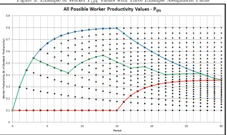
completed of a task. This effect is shown in Figure 2. Each curve represents a production plan
where 15 replications of the task are performed during 30 periods. The convergence of the curves
at period 30 indicates that the productivity in period 30 is the same regardless of when the 15
task replications were performed. Thus, at period 30, we need only know how many times the
task was done in the preceding 29 periods to calculate the current productivity. The reformulation
[image:24.612.89.517.437.672.2]technique, discussed later, is based on this fact.
Figure 2: Example Learning Curves for Sample Worker Under Different Task Assignments
task or minimize the time until due dates are met. Implementing the objective which attempts to
maximize every task’s output when in the presence of an unbalanced line and infinite buffer capacity
leads to poor product flow and overproduction in upstream tasks. An alternative objective function
which encourages cross-training is discussed in the next section.
3.3 Reformulation Technique
Hewitt et al. [2013] has identified a reformulation technique and applied it to worker
alloca-tion models with learning with promising results. The following subsecalloca-tions discuss the addialloca-tion
constraints and variables that transform the model from a Mixed Integer Non-Linear Problem to
a Mixed Integer Problem resulting in much more manageable solve times. For a more complete
discussion of the reformulation see Hewitt et al. [2013].
The basic concept of the reformulation says that if a non-linear equation has variables with a
finite and countable domain then constraints and binary variables can be added to represent that
non-linear equation without approximation. While it is used to address non-linear learning and
forgetting curves in this work, the general form of the reformulation can be applied to a vast array
of functions.
Consider the functionf(∗) which does not have to be non-linear but, again, non-linear functions
are of particular interest. Let g(Y) be a linear equation andY be a vector of binary variables. Let
g(Y) have a finite and countable domain contained in SetK. Consider the function r =f(g(Y))
which needs to be modeled with linear constraints and binary variables. Since g(Y) has a finite
and countable domain, f(g(Y)) has a finite and countable range which can be found through
enumeration. LetZk be a vector of binary variables that indicate which item kin SetK is chosen.
The addition of the following constraints complete the remodeling:
r=X
k∈K
f(k)Zk (11)
g(Y) =X
k∈K
kZk (12)
X
k∈K
Zk= 1 (13)
domain. Solving for 13,23, and 33 yields 1,8,and 27. With the addition of three binary variables
Z1, Z2,and Z3 and a constraint such that Z1+Z2+Z3 = 1 the equation X = 1Z1+ 8Z2+ 27Z3
can represent the original equation X = (g(Y))3. The original non-linear equation can then be
replaced with the two linear equations by adding the binary variables and constraints. The use of
the technique in this work to transform the model from a mixed integer nonlinear program to a
mixed integer program is explained below.
The productivity of a worker in a given period is a function of the number of replications he has
performed on a given task. The number of replications a worker could have performed,k, in a given
period t is of finite and countable domain, specifically k ∈ Z{1, .., t} as a worker could not have
performed a number of replications greater than the number of opportunities he had to perform
the task. Substituting possible values of kforPt
q=1Xijq in Constraint(10) yields the productivity of a worker ion a taskj in a period twho has done the taskk times (Pijtk).
Figure 3 shows all the possible productivity levels for an example worker. With the addition
of binary variables Zijtk we can reformulate the nonlinear Constraint (10) in the same way as the
above equationX = (g(Y))3. The necessary variables and constraints to perform the reformulation
Figure 3: Example of Worker Pijtk Values with Three Example Assignment Paths
3.3.1 Reformulation Variables & Parameters
The following variables and parameters are required for the reformulation.
Zijtk - binary - indicates if workerihas been assigned to taskj ktimes before and including period twhere k≤t∈ T
Pijtk - parameter precalculated outside of model following equation (14) - Productivity of workeri
who has performedkreplications on task j before and including period twherek≤t∈ T
Pijtk =Iij +Kij
1−exp
−1 Lijk
exp
1
Fij(k −t)
∀i∈ I, j ∈ J, t∈ T, k < t∈ T
(14)
3.3.2 Reformulation Constraints
The following constraints effectively replace constraint (10) using the reformulation variables and
parameters.
t
X
k=1
(k∗Zijtk)≤ t
X
c=1
Xijc ∀i∈ I, j ∈ J, t∈ T (15)
t
X
k=1
Zijtk =Xijt ∀i∈ I, j ∈ J, t∈ T (16)
Oijt≤Xijt∗M ∀i∈ I, j ∈ J, t∈ T (17)
Oijt≤Sj∗ t
X
k=1
(Zijtk∗Pijtk) ∀i∈ I, j ∈ J, t∈ T (18)
Oijt≥U∗Sj∗ t
X
k=1
(Zijtk∗Pijtk) ∀i∈ I, j ∈ J, t∈ T (19)
T
X
t=k
Zijtk ≤1 ∀i∈ I, j ∈ J, k∈ T (20)
The productivity of the worker is set as a parameter defined by the index k representing the
number of replications of worker i has performed task j by period t. Instead of solving the
ex-ponential function as a part of the optimization, the feasible values are passed into the model as
parameters calculated in constraint (14). Binary variables then decide which productivity values
are to be used at which times. The k index in the variable Zijtk represents the number of times
a worker has been assigned to a task as does the sum of Xijt over the time. Constraint (15)
ensures that values the chosen values of Zijtk correspond with the assignments up to the current
period. Without Constraint (15) workers would not follow their learning and forgetting curves.
Constraint (16) ensures that when worker i is assigned to a task j one of the variables Zijtk is
set high and when worker iis not assigned Constraint (16) ensures that no Zijtk takes on a high
value. Constraint (17) ensures that the X variables take values of 1 when corresponding worker
task standard production rate, the Z decision variable, and the productivity. Constraint (19) sets
the output of a worker to be greater than the product of the minimum worker utilization, the task
standard production rate, theZ decision variable, and the probability. Constraint (20) essentially
ensures that each worker can only perform a nth replication of a task once. For example, a worker cannot be assigned to a task for the 5th time more than once.
3.4 Practicing Reduction
The original model formulation allowed for the possibility that a worker be assigned to a
task but not produce anything. While workers do not produce any output, their assignment is
still included in the productivity calculations. Hence, they learn but do not produce anything,
so these events are refers to as practicing. Examine constraint (2) to see how a worker’s output
can be 0 while a worker is assigned to a task. Because the model uses experiential learning and
forgetting curves where learning is based on actual completion of a task, the presence of practicing
yields overestimate of a worker’s productivity since the learning curve assumes that workers always
produce as much as they can. Changing the inequality in Constraint (2) to an equal-to inequality
would eliminate the practicing, but would greatly restrict the flexibility of worker assignments.
The change would require workers to be 100% utilized during their assignments. In an unbalanced
line, requiring workers to be fully utilized makes assignments difficult and often makes lines less
productive. Because of the worker learning rate heterogeneity, perfectly balanced lines are seldom
seen, so a different solution is needed.
Constraints (18) and (19) in combination, aim to control practicing while setting a minimum
worker utilization. Constraint (18) sets the maximum productivity for a worker and Constraint
(19) ensures that if the worker has been assigned to the task his utilization on that task is at least
100∗U% of his maximum productivity at that time. Higher values ofU reduce worker “practicing”
which occurs when a worker is assigned to a task but performs the task less times than expected
but is counted as having learned an amount which corresponds with his maximum productivity.
A value of 0 forU could yield episodes of worker practicing, thus overestimating his productivity
in future periods. Alternatively, in the presence of an unbalanced line a value of 1.0 for U would
lead to poor product flow requiring assigned workers to be 100% utilized with zero waiting time
allowed. This leads to many periods where most workers are not assigned to any task as they
according to their worker utilization requirements. Constraint (20) also controls another possibility
of practicing. Without constraint (20) worker could repeat task replications. For example, a worker
could work steadily on a task for 5 periods, gaining skill following his learning curve and then, in
the next period, the worker could perform as though it was his first time being assigned on the
4
Research Strategy
In this section, we discuss how individual experimental factors will be included in the
analy-sis. The goal of this work is to demonstrate how the model can allocate workers to tasks under
different system structures. The model optimally allocates workers by maximizing the production
of demanded items while considering inventory constraints. How differing inventory constraint
structures affect optimal worker allocations and ultimately the productivity of the system has been
left unstudied due to problem size constraints observed when solving similar models with human
learning and forgetting Sayin and Karabati [2007]. The strategy used in this work is to run multiple
models with differing system configurations and compare the solutions. In this way, the effects of
work structure on cross-training can be better understood. The experiments will show how the
model could help managers of systems with various work structures better utilize their workforce.
4.1 Model Responses
To evaluate the performance of the model, two performance metrics are considered: the model
solution time and the production of the products in the system. The solve time of an experiment is
an important metric to track as anyone seeking to use the model needs to know how long the model
will likely take. Longer solve times are a concern for industrial use as production changes can occur
rapidly, requiring quick response. Solve times will be reported in seconds. The production of a
system is the second performance metric of interest. After model termination, the objective value
is reported which represents how many due dates were met and how much product the system
produced under the solution at the time of model termination. There may arise differences in
production due to due dates, worker set, or another design factor which need be explored.
4.2 Experimental Design Factors
The list of experimental factors follows:
1. The number of periods. This factor is set at 25 periods. While there is interest in using math programming models for long-term individual assignments, today’s firms face the need
to react quickly to things such as worker attrition, consumer demand changes, or new product
introduction. The planning horizon of the model is approximately one month and 25 periods
2. The number of tasks. This factor is set at 15 tasks. Hewitt et al. [2013] identifies this as a desirable increase from comparable studies. Larger increases in quantity of tasks yields
numerous possible work structures as more tasks can be performed in parallel. The chosen
level of tasks is closer to industrial examples and allows a multitude of structures and instances
to be tested.
3. The number of workers. This factor is treated at one level with 7 workers corresponding to a staffing level of 50%, identified as common in DRC systems by Molleman and Slomp
[1999], to gauge the effect of the worker-task ratio on performance metrics. The idea of using
less than full staffing levels is that DRC systems need to have fewer workers than machines
as the job shop type work done is these systems does not require work to be done on all the
machines at the same time. An increase in staffing level may decrease the amount of worker
multifunctionality seen in the solutions as workers will not need to rotate as often. Hewitt
et al. [2013] show that, surprisingly, as the number of workers increases, the problem becomes
easier to solve.
4. Worker Skill Mix. This is a group of factors which are generated together to create an heterogenous set of workers. Two randomly generated worker sets are tested for the
experiments to show how worker mix affects performance of the model.
(a) Worker Forgetting Rate. For each task, workers are assigned a random forgetting rate
between 10 and 35 where lower values represent faster forgetting.
(b) Worker Learning Rate. For each task, the workers’s learning rates are treated at a
random level between 2 and 10 where lower values represent faster learning.
(c) Worker Steady State Productivity. For each task, the workers are assigned are assigned
a random steady state productivity between 0.5 and 0.9.
(d) Worker Initial Productivity. For each task, the workers are assigned are assigned a
random initial productivity between 0.1 and 0.9.
5. Product Demand. The product demand quantity for each end product is assigned a value between 2 and 9. Larger demanded quantities will likely yield greater worker
mulitfunction-ality and lower task tenure while workers have to switch tasks more often to push product
6. Due Dates. Due dates and multiple products are being modeled following the logic presented in Corominas et al. [2010]. The differing product structures include those which have multiple
products which must be accounted for. A due date is considered to be met if the demand of
a product is fulfilled before the assigned due date which is between period 10 and period 25.
Not all due date are required to be met, but meeting due dates is highly desirable and given
high weight of 1000 in the objective function.
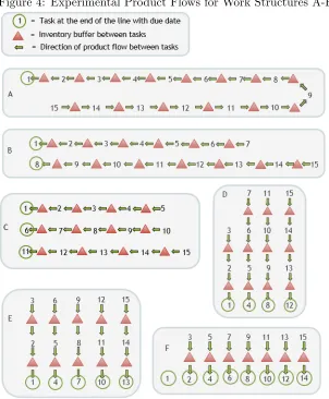
7. Work Structure. This factor is treated at multiple levels. Different structures may have a different number of end tasks with differing demands. A graphical representation of the
work structures can be seen in Figure 4 below. The number of units of output from task
j required to complete task j0 (Uj,j0∈ Parentsj) is also random between pairs of j and j0 for each work structure tested. Additionally, the standard production rate (Sj) which represents
the difficulty of a tasks is set to a random level of 1 or 2 for each task. Figures 4 and 5
show how product flows through the chosen experimental work structures (labeled A-K).
The structures do not encompass all the possible flows the model could be used to solve but
are used to demonstrate the flexibility of the implemented inventory constraints to cover a
larger set of systems than seen in the literature. Work structures A through F consist of
simpler linear production flows starting with a single flow in structure A and increasing to
eight parallel flows in structure F. These or very similar structures can be found in industry
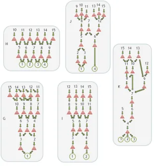
and vary the number of tasks that can be performed in parallel. Work structures G through
K are less common orientations of the same 15 tasks and are included to demonstrate the
robustness of the modeling method. Structures G through K include numerous instances of
tasks which require multiple inputs from other tasks, a characteristic seen in industry, but
seldom observed in the literature.
8. Task Standard Production Rate. To ensure that the production lines in the systems being tested are close to balanced the standard productivity rates for individual tasks are set
to be within ± 1-10% of the balanced line productivity rate. Imbalanced lines are avoided
because they yield results in which workers are often not allocated to tasks due to waiting
Figure 5: Experimental Product Flows for Work Structures G-K
4.3 Generation of Factor Random Values
Random values for the experimental factors are generated using the Python function randint().
The randint() function produces pseudo-random integers contained in the range passed during call.
The randint() function is part of the “random” library in Python and has roots in the random()
function which produces pseudo-random floats in the range (0.0, 1.0]. Both random() and randint()
use the Mersenne Twister, a widely used generator, at their core [van Rossum, 2011].
4.4 Algorithm Tuning
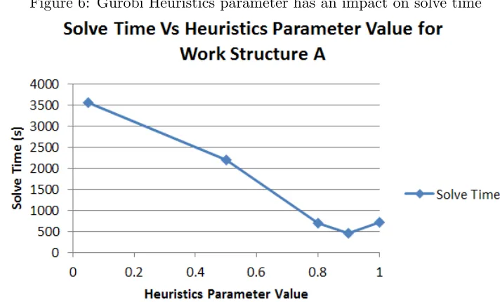
In implementing the model it may be necessary to adjust some solver settings to find better
solutions faster. Gurobi offers algorithm tuning tools which repetitively solve models under different
Because the solve times for the models in this work are so large, the standard Gurobi parameter
tuning tools were not considered. Some initial testing revealed that when the solver used a heuristics
solution, the optimality gap was decreased by finding a new incumbent solution. Experimentation
with Gurobi’s Heuristics parameter was found to have an interesting impact on the solve time of
the models as shown in Figure 6. For Work Structure A, the best performing level tested for the
[image:36.612.124.480.212.427.2]Heuristics parameter was 0.9 and thus was used for the rest of the experimental testing.
Figure 6: Gurobi Heuristics parameter has an impact on solve time
Computational Environment
To study the computational effectiveness of the model, the instances of the experimentation
were solved using Gurobi 5.1 to a relative optimality tolerance of 0.75% or an absolute optimality
tolerance of 7. Prior testing pointed to these tolerances to balance model solve times and solution
quality. Experiments were performed on a computer cluster where each node has 32-64 cores with
AMD Opteron 2.2 GHz or AMD Interlagos 2.6 bulldozer processors and 128-256 GB of memory.
For experimentation, the model instances were run on 6 cores with 24 GB of memory. When solving
each instance of the model, Gurobi was given a time limit of 15 hours.
Model Investigations
first experiment is an exploratory experiment which is meant to demonstrate the flexibility of the
model. The second experiment is 24 factorial experiment which is meant to explore how system
[image:37.612.167.448.165.350.2]structure, product demand, product due dates, and worker sets affect the model responses.
Table 3: Experimental Design
Factors Factor Levels
Experiment 1
Worker Skill Mix Worker Set 1
Product Demand Random ∈{2..9} for each product Due Dates Random Period ∈{10..25}
Work Structure All 11 Work Structures∈{A..K}
Experiment 2
Worker Skill Mix Worker Sets{1,2}
Product Demand Demand∈{3,8} for each product Due Dates Periods{12,22} for each product Work Structure Work Structures{A, J}
5
Results
Table 4 shows a sample allocation solution for Structure A taken from the algorithm tuning
Table 4: Sample Solution for Structure A
Worker
0 1 2 3 4 5 6
Period Tasks
1 7 13 14 8 9 6 15
2 7 13 2 8 10 11 15
3 7 5 3 12 9 11 15
4 4 5 14 8 10 9 15
5 7 13 14 12 3 9 1
6 7 13 14 8 10 2 1
7 4 13 2 12 3 11 1
8 4 13 2 12 10 6 15
9 4 5 14 12 3 9 1
10 7 13 14 8 3 9 11
11 4 13 14 8 10 9 11
12 7 5 11 12 10 6 15
13 7 13 2 12 15 6 11
14 12 13 14 11 3 6 15
15 4 5 14 8 3 9 11
16 4 5 14 12 10 9 11
17 4 5 2 11 3 6 1
18 7 5 2 8 10 6 1
19 4 13 2 12 10 9 1
20 4 5 2 8 3 6 9
21 7 5 2 12 10 6 11
22 4 1 2 12 3 9 15
23 7 13 2 11 3 6 1
24 4 5 14 8 3 15 1
Workers perform and focus on between 2 and 3 tasks throughout the planning horizon. With a
staffing level of 50%, that level of worker multifunctionality is to be expected.
To contrast Table 4, Table 5 shows a sample allocation solution for Structure J observed during
Experiment 2 that shows the differences between the allocations for two work structures. The
model was run to an absolute optimality gap of 7 units. The chosen gap is used for the experiments
because it was found to allow the models to solve in a reasonable amount of time while producing
Table 5: Sample Solution for Structure J
Worker
0 1 2 3 4 5 6
Period Tasks
1 12 14 15 5 6 11 13 2 12 14 15 9 6 7 13 3 8 14 15 4 6 7 13 4 12 14 15 4 6 10 13 5 8 14 15 4 6 7 13 6 12 14 15 4 6 3 13 7 12 14 15 4 6 7 13 8 12 14 15 4 6 2 13 9 12 14 2 4 6 1 13 10 12 14 15 4 6 10 13 11 12 14 15 4 6 3 13 12 12 14 15 4 6 9 13 13 1 14 15 9 6 7 11 14 12 14 15 4 6 7 13 15 12 14 15 5 6 7 13 16 12 14 15 4 6 1 13 17 12 14 15 4 6 1 13 18 12 2 15 4 3 1 13 19 12 14 15 4 6 13 11 20 12 14 15 5 6 4 13 21 NONE 8 2 4 11 7 13 22 NONE 3 15 NONE 6 10 11 23 NONE 8 15 9 6 7 2 24 5 NONE NONE 4 12 10 8
Compared to the solution seen in Table 4, some workers perform and focus on fewer tasks
throughout the planning horizon. Additionally, worker multifunctionality is not evenly distributed
across the workers. Many workers focus on a single task while Worker 5 performs many tasks.
This result may be because the production route to task 4 is simpler than that to task 1, causing
more work to be done on tasks 13,14,15,12,and 6. Use Figure 5 for reference of structure J. There
also seems to be significant end of period effects in this sample result for structure J. In particular,
worker allocations follow a steady pattern up until the last few periods. The end of period effects
are an artifact of the model formulation and effort could be taken in future work to eliminate them.
5.1 Experiment 1
Figure 7 plots the solution times after relative optimality gap was reduced to under 0.75% reported
Figure 7: Solve time results for Experiment 1
We observe that Gurobi, given most of the tested work structures, is able to produce quality
solutions in reasonable time frames. However, the cases with the most complex structures with
many parallel tasks, I and J, take the longest to solve. Interestingly, the case with work
struc-ture K, which is similar to I and J, was solved in a similar amount of time as many of the other
cases. The case with work structure B took longer than anticipated. While work structure B has
two parallel lines, not too different from work structure A, C, or D, the case was required much
more time to find an optimal solution than other, similar cases. Interestingly, all three structures
that took longer to solve than other structures had 2 products. It may be the case that the long
production lines paired with the multiple due dates for the products are driving up the solution
times. While structure K does have long production lines and three products, the products are
dates on structure J is explored further in Experiment 2.
[image:41.612.116.484.155.504.2]Figure 8 reports the average units produced per product line for the cases tested in Experiment 1.
Figure 8: Production results for Experiment 1
Work structures A through D have very similar average values, while cases with work structure
E through K have different average values of production. A replication of the experiment may show
that the variation in production may be due to the random standard production rates.
Table 6 - 14 represent the solutions generated in Experiment 1. Tables for Structures I and J
Table 6: Experiment 1 Solution for Structure A
Worker
0 1 2 3 4 5 6
Period Tasks
1 14 10 2 8 4 3 15
2 14 5 13 7 6 9 4
3 15 12 13 7 5 11 1
4 4 12 13 8 3 9 2
5 14 5 NONE 12 6 11 15
6 4 11 13 8 15 7 1
7 4 12 13 10 14 5 15
8 5 7 13 10 1 6 9
9 10 NONE 2 14 6 5 3 10 4 9 11 8 NONE 5 12 11 7 10 NONE 14 4 5 12
12 2 4 NONE 11 6 9 3
13 4 5 2 8 11 9 3
14 12 1 2 14 NONE 13 3 15 2 15 NONE 8 10 7 11 16 NONE 7 3 15 6 10 NONE
17 2 9 11 8 6 13 1
18 2 13 9 10 3 NONE 1
19 2 4 11 3 10 13 1
20 15 7 3 14 9 NONE 12 21 15 12 NONE 14 6 7 11 22 1 11 3 15 NONE 5 12
23 4 5 2 14 11 13 10
24 1 12 5 8 9 13 3
Table 6 represents the assignment solution for work structure A in Experiment 1. Every worker
except worker 3 is not assigned to a task in at least one period and perform many of the same
Table 7: Experiment 1 Solution for Structure B
Worker
0 1 2 3 4 5 6
Period Tasks
1 4 15 2 8 3 13 11 2 4 5 2 14 13 9 15 3 4 5 13 12 14 6 11 4 1 10 13 12 15 9 4 5 7 15 10 5 3 6 14 6 12 7 2 5 3 6 11 7 4 11 13 14 9 7 1 8 12 7 13 14 3 6 11 9 10 7 14 5 3 6 9 10 15 10 2 5 3 7 4 11 14 7 15 5 3 6 1 12 7 10 11 12 15 9 1 13 4 9 13 5 3 12 1 14 4 5 2 14 3 6 13 15 7 5 2 8 14 6 1 16 4 10 2 5 15 6 11 17 4 7 13 8 3 6 14 18 12 10 13 8 7 9 1 19 7 11 2 8 15 6 12 20 4 5 7 8 3 6 1 21 14 5 13 10 3 9 4 22 15 5 10 12 7 6 11 23 7 5 13 8 15 9 1 24 14 11 2 8 15 9 12
Table 7 represents the assignment solution for work structure B in Experiment 1. Unlike
the solution for work structure A, in the solution for structure B workers do not have periods of
inactivity. Workers also exhibit longer average task tenure and perform fewer tasks than in the
Table 8: Experiment 1 Solution for Structure C
Worker
0 1 2 3 4 5 6
Period Tasks
1 14 5 13 11 10 8 15
2 14 7 9 12 10 8 15
3 14 13 2 12 10 3 15 4 15 14 13 4 10 8 9
5 7 10 2 12 8 3 1
6 13 7 5 NONE 9 8 11
7 5 11 8 9 15 4 1
8 4 13 5 14 3 11 1
9 2 13 14 12 8 9 1
10 NONE 5 13 12 9 4 8 11 13 7 10 11 15 4 14 12 2 3 13 12 15 6 11
13 1 5 8 2 6 3 15
14 NONE NONE 8 11 15 3 1 15 4 5 8 12 6 NONE 3
16 6 5 11 2 9 7 3
17 4 1 11 15 3 13 12 18 NONE 3 8 NONE 4 11 2
19 5 3 14 10 6 4 8
20 NONE 7 8 11 14 6 9
21 7 13 8 5 9 4 1
22 14 7 13 12 6 8 10 23 8 NONE NONE 11 1 4 2
24 15 5 14 11 3 9 2
Table 8 represents the assignment solution for work structure C in Experiment 1. Many workers
Table 9: Experiment 1 Solution for Structure D
Worker
0 1 2 3 4 5 6
Period Tasks
1 7 13 2 9 3 11 1
2 14 13 2 8 3 11 1
3 9 10 2 5 3 8 1
4 6 10 2 NONE 3 11 1
5 12 7 2 11 3 9 1
6 6 5 2 10 3 11 1
7 5 1 2 NONE 3 9 11
8 5 10 2 8 3 14 15
9 7 10 14 8 3 9 1
10 7 10 2 NONE 3 8 15
11 12 NONE 13 8 3 9 4
12 6 1 13 8 3 9 15
13 4 NONE 2 5 3 6 1
14 15 12 NONE 5 8 NONE 4 15 4 NONE NONE 10 1 11 2
16 4 12 NONE 5 1 7 2
17 4 NONE NONE 5 6 NONE 1 18 14 1 2 NONE 13 11 3
19 1 9 2 NONE 6 8 NONE
20 5 9 2 NONE NONE 8 1 21 NONE NONE 2 NONE 9 7 1
22 14 5 2 NONE 11 8 1
23 NONE 2 5 10 4 6 3
24 NONE 3 2 15 1 7 4
Table 9 shows the results for structure D which, out of all of the solutions, shows the most
periods when workers are not assigned to any task. Unlike in the previous solutions workers perform
Table 10: Experiment 1 Solution for Structure E
Worker
0 1 2 3 4 5 6
Period Tasks
1 9 5 2 8 3 4 1
2 9 NONE 2 8 3 4 1 3 9 NONE 2 8 3 13 1 4 9 NONE 2 8 3 6 1 5 9 NONE 2 7 3 5 1
6 9 7 2 8 3 5 1
7 NONE 14 2 8 3 10 1 8 15 12 2 7 3 10 1 9 13 6 2 5 3 NONE 1 10 15 11 2 5 3 6 1 11 12 7 14 15 3 13 1 12 14 9 2 NONE 3 13 1
13 12 7 2 8 3 4 1
14 15 13 2 7 3 11 1 15 14 10 2 NONE 3 NONE 1 16 15 NONE 2 7 3 13 1 17 15 11 2 NONE 3 13 1 18 14 NONE 2 11 3 7 1 19 NONE NONE 2 11 3 13 1 20 14 9 2 8 3 NONE 1 21 13 1 2 10 3 9 4 22 7 9 2 10 3 NONE 1 23 12 1 2 15 3 5 4 24 14 7 2 15 8 6 1
Table 10 represents the assignment solution for work structure E in Experiment 1. Workers
2, 3, and 6 perform primarily only one task and because of that, the solution for structure E has
the lowest average values for task redundancy and worker multifunctionality and highest value for
Table 11: Experiment 1 Solution for Structure F
Worker
0 1 2 3 4 5 6
Period Tasks
1 9 13 2 8 15 11 1
2 9 13 5 8 10 4 1
3 9 12 11 8 15 7 1
4 9 13 14 8 3 11 1
5 9 12 11 8 3 4 1
6 14 5 11 7 10 4 1
7 9 13 2 7 3 11 1
8 9 12 2 8 10 5 1
9 14 13 12 8 4 NONE 1 10 14 13 6 10 15 11 1 11 7 5 14 2 15 NONE 1 12 6 12 14 10 15 11 1 13 4 13 NONE 10 15 3 1 14 NONE 12 2 11 6 3 1 15 14 12 3 10 15 13 1
16 4 5 3 11 15 6 1
17 14 12 2 10 NONE 4 1 18 2 9 5 10 12 NONE 1
19 4 11 3 8 6 5 1
20 10 5 3 NONE 6 11 1 21 2 15 14 11 6 7 1 22 11 2 3 9 10 NONE 1 23 NONE 13 2 11 10 NONE 1 24 9 11 15 10 3 7 1
Table 11 represents the assignment solution for work structure F in Experiment 1. The solution
shows workers assigned to their initial tasks for multiple periods and worker 6 only assigned to task