White Rose Research Online URL for this paper:
http://eprints.whiterose.ac.uk/83611/
Version: Accepted Version
Proceedings Paper:
Saat, FAZM and Jaworski, AJ (2013) Oscillatory flow and heat transfer within parallel-plate
heat exchangers of thermoacoustic systems. In: Proceedings of the World Congress on
Engineering 2013. Lecture Notes in Engineering and Computer Science. World Congress
on Engineering 2013, 3-5 July 2013, London, UK. Newswood Limited , 1699 - 1704. ISBN
9789881925299
eprints@whiterose.ac.uk https://eprints.whiterose.ac.uk/ Reuse
Unless indicated otherwise, fulltext items are protected by copyright with all rights reserved. The copyright exception in section 29 of the Copyright, Designs and Patents Act 1988 allows the making of a single copy solely for the purpose of non-commercial research or private study within the limits of fair dealing. The publisher or other rights-holder may allow further reproduction and re-use of this version - refer to the White Rose Research Online record for this item. Where records identify the publisher as the copyright holder, users can verify any specific terms of use on the publisher’s website.
Takedown
If you consider content in White Rose Research Online to be in breach of UK law, please notify us by
Abstract—Oscillatory flows past solid bodies are a feature typical for thermoacoustic systems. Understanding such flows is one of the keys for improving the system performance. This work investigates oscillatory flows around parallel-plate heat exchanger through numerical modeling developed based on the experimental data obtained in-house within a standing-wave thermoacoustic setup. Attention is given to developing a model that can explain the physics of phenomena observed in the experimental work. Four drive ratios (defined as maximum pressure amplitude to mean pressure) were investigated: 0.3%, 0.45%, 0.65% and 0.83%. The suitability of selected turbulence models for predicting the flow phenomena at varied drive ratios has been tested. Discussion of results is based on the velocity profiles and vorticity contours within the flow. Associated heat transfer phenomena are also discussed.
Index Terms—parallel-plate heat exchanger, turbulence, transition, oscillatory/thermoacoustic flows.
I. INTRODUCTION
scillatory flows around solid bodies are a typical feature in thermoacoustic systems. These are developed based on a thermoacoustic effect which occurs when an acoustic wave interacts with a solid boundary in the presence of temperature gradient, and which produces cooling effects or generates acoustic power when a suitable phasing between pressure and velocity occurs. Comprehensive reviews on thermoacoustics can be found in [1]. Thermoacoustic technologies are attractive due to the lack of moving parts in the thermodynamic process, which makes them simple, reliable and inexpensive.
The oscillatory flow around the internal structures of thermoacoustic systems has been investigated in various experimental and numerical works. Several interesting features were discussed including the evolution of vortex structures at the end of plates [2], entrance effect [3], flow structures between stack plates [4] and viscous dissipation [5], to name but a few. Theoretical [1] and numerical works (cf. [5]), related to thermoacoustic processes, typically
Manuscript received March 05, 2013; revised April 05, 2013. F. A. Z. Mohd Saat would like to thank the Government of Malaysia and Universiti Teknikal Malaysia Melaka, Malaysia for sponsoring her studies.
F. A. Z. Mohd Saat is with the Department of Engineering, University of Leicester, University Road, LE1 7RH United Kingdom, on leave from Universiti Teknikal Malaysia Melaka, Malacca, Malaysia (email:fazms1@le.ac.uk)
A. J. Jaworski is with the Department of Engineering, University of Leicester, University Road, LE1 7RH, United Kingdom (corresponding author; phone: +44(0)1162231033; fax: +44(0)1162522525; e-mail: a.jaworski@le.ac.uk).
assume a laminar flow (limited to very low drive ratios). The critical Reynolds numbers for transition to turbulence in an oscillatory flow were reviewed in [6]. The experimental results of [6] agree with the critical Reynolds number, Rec=2um/( 2 f)1/2=400, suggested by [7], with um, and f
representing the velocity magnitude at the center of pipe, kinematic viscosity and frequency, respectively. The flow regions were categorized as laminar, transitional and turbulent. However, oscillatory flows of Rec higher than 400
were shown experimentally [8] to experience a stage of relaminarization where the velocity profiles match the laminar prediction during the initial stage of the acceleration phase and change to turbulent-like profiles at the later phase, before turning back to laminar. An additional complication in the transition/relaminarization processes will be the appearance of temperature dependencies in fluid properties, compressibility effects, or additional forces such as gravity [9]. The presence of temperature field was shown experimentally to cause asymmetry to the flow [10]. Natural convection effects were also observed [11]. The heat loss has been numerically estimated through the introduction of a heat sink/source to obtain the heat transfer predictions close to experiment [12]. This approach gave a general idea about the magnitude of heat losses occurring in the experiment. Detailed investigation is needed to identify the mechanism that contributes to these losses. The natural convection was shown to have a small effect on the flow and heat transfer of the previous investigation [13]. Here, the influence of flow drive ratio on the fluid mechanics and heat transfer processes will be presented.
II. COMPUTATIONAL MODELING
A. Transport Equations
The numerical calculations are carried out by solving the appropriate transport equations that govern the flow. For brevity, the equations are shown in index notation [14, 15]: Continuity equation;
0
i j
u x
t
(1)
Momentum/Reynolds Equation;
ui Smi x j u i u j x
ij j x i F i x
p j
u i u j x t
i u
2 ' '
'
(2)
Energy equation;
Oscillatory Flow and Heat Transfer Within
Parallel-plate Heat Exchangers of Thermoacoustic
Systems
Fatimah A.Z. Mohd Saat and Artur J. Jaworski
ui
ij eff Shj x T eff k j x p E i u i x E t
, (3)
where 2 2 i p u p T c E
(4)
ijk k j i i j ij x u x u x u 3
2 . (5)
Here subscripts i,j=1,2,3 correspond to the components of x, y and z respectively. The terms , u, p, t, F, cp, k, E and ij
represent the density, velocity, pressure, time, external force, heat capacity, thermal conductivity, internal energy and stress tensor, respectively. All terms correspond to the values of mean flow except the fluctuating components, u’i,j,
also known as Reynolds stresses. The effective stress tensor (ij)eff has the same formulation as equation (5) but with the
mean viscosity, , replaced by the effective viscosity,
eff= + t. Similarly, the effective thermal conductivity,
keff=k+kt replaces k. Turbulent thermal conductivity is
calculated as, kt= tcp/Prt and turbulent Prandtl number, Prt.
has a constant value of 0.85. The eddy viscosity, t, is
calculated using turbulence model. The terms Sm and Sh are
the user-defined features available in ANSYS FLUENT 13. Note that, equations (1)-(3) represent the transport equations of the form of Reynolds-averaged Navier-Stokes (RANS) equation for turbulent flow. For a laminar flow, the momentum equation has a similar form to equation (2) but without the Reynolds stresses term ( ui’uj’ and ui’2).
Similarly, the energy equation representing laminar flow is solved using equation (3) but with the absence of turbulent contribution ( t and kt) in the effective viscosity, eff, and
effective thermal conductivity, keff. The equation governing
laminar flow was also presented in [13]. The Reynolds stresses are solved through additional equations provided by the turbulence model. Turbulence is assumed isotropic so that Boussinesq hypothesis is applicable to relate the Reynolds stresses to the mean velocity gradient as follows:
ij k k t i j j i t j i x u x u x u u
u
k 3 2 ' ' (6)
The term, k=(u1’2+u2’2+u3’3)/2, is known as the turbulent
kinetic energy. The Kronecker delta, ( ij=1 if i=j and ij=0 if
ij) was introduced to correctly model the normal
component of the Reynolds Stress [14]. Several RANS turbulence models were tested in this study. It was found that a four-equation transition Shear-Stress Transport (SST) model and a two-equation SST k- model were the most suitable for the flow investigated. These additional equations were introduced to solve for turbulent viscosity,
t, and turbulent kinetic energy, k, to obtain the
Reynolds-stresses using equation (6). The details of the additional equations and related empirical constants for SST k- and transition SST are defined in [16] and [17], respectively. The values for all empirical constants proposed in both papers are retained for the study. For the internal flow, small modifications were made to two of the constants in transition SST model following suggestion from [18]. The equations are solved with an application of appropriate setting in commercial software ANSYS FLUENT 13.
B. Physical Domain
The computational domain used in this study is based on the experimental setup presented in [11]. The domain covers the full height of the test section with multiple-plate area as in the experiment. In previous investigation [13], a two
dimensional model covering the full length and height of the experimental setup was developed. The model was shown to give good predictions of flow structures for a drive ratio of 0.3%, in agreement with experiment [13]. The full length model allows the verification of the phase changes between pressure and velocity from the computational model to follow the definition from the experiment. It was also found that the pressure and velocity in the flow far away from the heat exchanger can be estimated fairly well by the linear thermoacoustic theory. This indicates that the use of a shorter model is also acceptable provided that the boundary is far enough for the incoming/outgoing oscillatory flow not to interfere with plate structure [5, 14]. In this study, the computational domain was developed to cover a length of 270 mm either way from location m of the joint, as shown in
Fig. 1
Due to flow asymmetrycaused by the natural convection as observed in [13], the height is set to 86 mm to cover all the 10 parallel-plates used in the experiment. The selection of short model is favorable because it is computationally less expensive than the first model that covers the full length of the two-dimensional area.
C. Solver selection and boundary conditions
Laminar model was solved using Navier-Stokes equation and RANS equation was used for turbulence model. A pressure-based solver was used for all models with the application of Pressure-Implicit with Splitting Operators (PISO) algorithm for the pressure-velocity coupling. Second order discretization was selected for discretization of time, transport equation and turbulent equations. The boundary conditions were calculated from the lossless equation [1, 12] and given as:
kax ft
a P
P1 cos 1cos2 (7)
kax ft c
a P
m'2 sin 2 cos2 (8)
Fig. 1. Schematic diagram of the experimental setup and the selected computational domain (top); meshed area of the computational domain (middle); enlarged view of the area for plotting velocity profiles and vorticity contour (bottom).
[image:3.595.289.542.51.295.2]0 . 2 1
x x x
T (9)
Oscillating pressure, P1, and mass flux, m’2, are assigned at
locations x1 and x2, respectively. These are shown in Fig. 1.
The wave number, ka=2 f/c, is constant because frequency,
f, is fixed at 13.1 Hz. The terms c and Pa refer to speed of
sound and oscillating pressure measured at pressure antinode, respectively. The phase, , is set to follow the standing wave criterion where pressure and velocity are 90
out of phase. Condition (9) was set at boundaries x1 and x2
so that when the flow reverses, the temperature of the reversed flow is equal to the temperature of cells next to the boundary. The temperature at the heat exchanger wall has a profile taken from measurements [11]. The resonator walls are adiabatic. The mean pressure was set to 0.1 MPa. Nitrogen was used as the working medium and was modeled as an ideal gas.
A
seventh order polynomial equation [19] was selected to model temperature-dependent mean thermal conductivity, k, while thetemperature-dependent mean viscosity, , follows a power law model [1]. The influence of gravity was modeled with gravitational acceleration set to 9.81 m/s2. Additional boundary
conditions for turbulence model were set at the boundaries,
x1 and x2, by assigning a value of turbulence intensity, I, and
turbulence length scale, l, defined as:
Re 18
16 . 0
'
a ver a ge
u u
I (10)
D
07 . 0
l (11)
The Reynolds number, Re= umD/ , is calculated using
velocity at location m, um, obtained from [11] and the gap
between plates, D = 6 mm, as shown in Fig. 1. The density,
, and viscosity, , used in equation (10) were taken at 300K.
The sensitivity of the results to these inlet conditions was tested by changing the value of turbulence intensity, I, to be
the value calculated using velocity at the boundaries. The velocity at the boundaries was calculated using equation from lossless theory. It was found that the solution is insensitive to the turbulence boundary conditions. This shows that the computational domain is sufficiently long to avoid the interaction between the flow around the plates and the inlet/outlet flows into/out of the domain.
[image:4.595.302.544.50.228.2]The solution was also tested for grid independency. Three mesh densities were tested: 37620, 45910 and 52830 elements. The medium mesh density of 45910 was found sufficient to provide grid independent solution. As seen in Fig. 1, the mesh density is higher near the wall, plate edges and within the area near the joint, with an increase ratio of 1.1. Analysis was done after the flow reached a steady-oscillatory state. In this study, it was defined as a state where pressure and velocity did not significantly change from one cycle to another. This was done by monitoring the pressure and velocity at location x2 as shown in Fig. 2. It
was found that the steady-oscillatory state based on the monitored pressure and velocity was achieved after 7 cycles. However, the iteration was continued until 70 cycles to reach a steady oscillatory-state in the temperature field.
The steady oscillatory state in temperature is defined as a state where temperature profiles are similar to experiment. As seen in Fig. 3 the temperature keeps a steady profile starting at 70 cycles onwards. The maximum time needed
for the iterations to reach 70 cycles is 180 hours (7 days) using a supercomputer with four-core AMD Opteron CPU’s running at 2.3Hz and 16 GB RAM. Fig. 3 shows that even at 490 cycles, the magnitude of temperature profile is still far from experiments. Reaching the state similar to experiment will be computationally very time consuming. The iterations are stopped at 70 cycles assuming steady-oscillatory state is achieved as the profiles shows similar trend to experiment. Prior to this decision, several attempts were made to investigate the possibility of setting the initial temperature to a value, T=300 K, or profiles, T=T(x,y),
[image:4.595.307.547.253.431.2]closer to experiment. However, the implementation of the initial profile leads to ambiguities especially related to the
Fig. 3. Temperature in the open area, 38mm next to the hot heat exchanger
Fig. 4. A relationship between pressure, velocity and gas displacement for twenty phases of a flow cycle.
[image:4.595.325.531.455.600.2]
Fig. 2. Pressure and velocity monitored at boundary x2.
difficulties in matching the natural convection effects. Hence, current model was initialized at 300 K and run for 70 cycles instead. The convergence was set to 10-4 for all
the transport equations. The calculation was carried out with a time step of 1/1200f.
In this paper, the phase is defined according to Fig. 4. Phase 1 was set for the maximum value of the oscillating pressure at location x2. All other phases follow by equally
dividing a flow cycle to 20 phases.
III. RESULTS AND DISCUSSION
A. Oscillatory flow without the influence of temperature
Initially, the flow was modeled using laminar model. The validity of the model was first tested with the heat exchanger surfaces set as adiabatic. The resulting velocity profiles between the heat exchanger plates agree very well with experimental data (cf. Fig. 5).
Fig. 6 shows the vorticity contour plotted for selected
phases representing the acceleration and deceleration of the oscillatory flow during the stage of suction and ejection.
The contours were plotted within the heat exchanger plates similar to the “viewing area” in the experiment [11], also shown in Fig. 1. During suction stage, from 1 to 10, the fluid is flowing in the positive direction into the plates, as defined in Fig. 4. The flow reverses at the ejection stage defined from 11 to 20. The vorticity, , from the numerical model is calculated as:
y u x v
(12)
Where, u and v are the velocity component in the x and y
direction of the flow. Fig. 6 shows the flow evolution within one cycle. A small vortex appears at the end of plates as flow starts to flow into the channel at 1. The vortex gets weaker as it moves into the channel and disappears completely before 8. A similar feature appears at the other end of the channel when the flow changes direction at 11. The laminar model was shown to capture well the features of the oscillatory flow at 0.3% drive ratio.
B. Oscillatory flow with the effect of temperature
The laminar model was then applied to the flow with the heat exchanger walls set at a constant temperature profile obtained by fitting the experimental measurement of temperature at the heat exchanger’s wall [11]. Fig. 7 shows the velocity profiles in selected phases for a flow with a drive ratio of 0.3%.
The comparison was done at 10 mm away from the joint above the cold heat exchanger as indicated in Fig. 1. In general, the velocity profiles calculated from the numerical model have the same shape to the experimental profiles. The maximum difference in magnitude is 0.03 m/s, equivalent to a 5% error compared to experiment. The flow was also modeled using transition SST and SST k- to check possible phenomena of transition or turbulence in the flow. All models appeared to give similar profiles. Laminar model was shown sufficient to model the flow at 0.3% drive ratio.
The velocity measured near the wall suffers from the uncertainty caused by thermophoresis of the seeding particles [20]. The thermophoretic force causes the particles to move away from the wall. The seeding particles also migrate away from the joint. For this reason, a comparison of vorticity plot between the plates cannot be done across the whole channel due to some of the experimental velocity data missing.
Fig. 8 shows the velocity profiles for flow modeled at drive ratios of 0.45%, 0.65% and 0.83%. It was found that transition SST model was the best for 0.45% drive ratio, giving the best predictions of the velocity profiles. For a higher drive ratio of 0.65% turbulent model appeared to be the best. It also gives a good agreement with experiments
[image:5.595.45.291.265.637.2]Fig. 5. Axial velocity profile plotted at 10mm away from the joint above cold heat exchanger at a drive ratio 0f 0.3%.
Fig. 7. Axial velocity profile plotted at 10mm away from the joint above cold heat exchanger at a drive ratio 0f 0.3%.
[image:5.595.50.288.267.438.2] [image:5.595.310.548.282.468.2] [image:5.595.46.290.450.637.2]
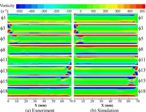
for 0.83% drive ratio. Vorticity contours calculated from both laminar and turbulent model are shown in Fig. 9, together with experimental results for comparison. Laminar model predicted that the flow disturbance was strong between the plates. The disturbance crosses the location 10 mm away from the joint causing changes to velocity profile at 8 as shown in Fig. 8(c). Turbulent model dissipates the kinetic energy of the flow to give a velocity profile similar to experiment. The resulting vorticity contours from the turbulent model were closer to experiment than those predicted by the laminar model.
All the drive ratios investigated in this study correspond to a critical Reynolds number, Rec, less than 400. The need for
using turbulent models was not expected. The resulting velocity magnitudes at location m for all the drive ratios
investigated are tabulated in table I. It is shown that the laminar model is sufficient to model the flow at 0.3% drive ratio. Transition model gave better predictions for 0.45%
drive ratio, but the difference in magnitude is not much improved. Turbulent model gave a very good comparison to experiment for 0.83% drive ratio. The profiles of velocity for drive ratio 0.65% were well estimated by the turbulent model, but the difference in magnitude is quite significant.
The velocity magnitudes tabulated in table I can also be used to represent the gas displacement, =um/2 f. It follows
that the drive ratios of 0.3%, 0.45%, 0.65% and 0.83% correspond to the gas displacement of 16, 23, 36 and 47 mm, respectively. Clearly, the gas particle in the flow with drive ratio higher than 0.65% moves more than half of the total length of the heat exchanger channel (70 mm). Then the flow reverses and moves over an approximately similar distance. The forward and backward movements of the gas particle bring the energy of the vortex structures at the end of plates into the channel. Vortex structures of a selected phase, 8, are shown in Fig. 10 for drive ratios of 0.3% and 0.83%. Clearly, the vortex strength for the wake appearing at the end of plates for 0.83% drive ratio can create a strong disturbance when it is pushed back into the channel. This could be a possible explanation for the appearance (and the need for) turbulence in this drive ratio as a means of dissipating the flow energy.
The disturbance is also complicated by the effect of thermal expansion that causes the gas particle to move at different magnitude for two halves of one cycle as suggested in [13]. Note that the critical Reynolds number, Rec, suggested in the literatures is obtained for a fully
developed flow in a relatively long pipe. The short length of the plates investigated here prohibits the flow of high drive ratios to reach a fully developed region. Most heat exchangers are short and a practical system works with high drive ratio. This study suggests that turbulence is likely to
(a) Experiment
(b)Laminar model
[image:6.595.56.510.51.538.2](c) SST k- model
Fig. 9. Vorticity contour from (a) experiment, (b) laminar model and (c) SST k- model between the heat exchanger’s plates at 0.83% drive ratio.
TABLE I
COMPARISON OF VELOCITY AMPLITUDE BETWEEN NUMERICAL MODELS Drive ratio Velocity amplitude at point m, (m/s)
(%) Experiment Laminar Transition SST SST k-w
0.3 1.30 1.32 1.32 1.32
0.45 1.90 1.99 1.98 2.00
0.65 2.97 3.07 2.86 2.84
0.83 3.84 4.40 - 3.73
(a)
(b)
[image:6.595.49.291.66.538.2](c)
occur within heat exchangers of high performance systems working in oscillatory flow condition.
C. Heat transfer
Finally, the wall heat transfer calculated from the model was compared to the experimental data. Heat flux, q, for all
models was averaged over horizontal length, x, and phase,
, and calculated as:
dxd
l
wa ll dy dT k l c h
q
2
0 0 2
1
, (13)
The subscript c and h refers to cold and hot heat exchanger,
respectively. Here, the mean thermal conductivity, k, was
used to calculate the heat flux obtained from laminar, transition SST and SST k- model [15]. Reynolds number is calculated as Re= umD/ .
Fig. 11 shows that the heat flux predicted from the numerical models and experiments increases with an increase of drive ratio. The Reynolds number calculated from the turbulent model was consistently closer to experiment with a good match of velocity discussed earlier. Turbulent model brings the magnitude of heat flux slightly closer to experiment.
IV. CONCLUSION
Whilst turbulent model was shown to predict the velocity profiles for a flow with drive ratio higher than 0.45% better, the prediction of heat transfer is still not satisfactory, particularly at cold heat exchanger working at drive ratio of 0.65% and 0.83%. Investigation on the turbulent heat transfer model could be something interesting to explore. It is also worth noting that modeling heat accumulation through proper initialization procedure may also be the solution. Nevertheless, the trend qualitatively agrees with experiment.
ACKNOWLEDGMENT
F. A. Z. Mohd Saat would like to acknowledge the support and technical contributions from Dr. Xiaoan Mao at the University of Leicester. The numerical modeling was done using the SPECTRE and ALICE High Performance Computing Facility at the University of Leicester.
REFERENCES
[1] G. W. Swift, “Thermoacoustics: a unifying perspective for some engines and refrigertors”, Acoustic.Soc.Am., 2002.
[2] X. Mao, and A. J. Jaworski, “Application of particle image velocimetry measurement techniques to study turbulence characteristics of oscillatory flows around parallel-plate structures in thermoacoustic devices”, Meas. Sci. Tech. 21, 2010, 035403.
[3] A. J. Jaworski, X. Mao, X. Mao and Z. Yu, “Entrance effects in the channels of the parallel plate stack in oscillatory flow conditions”,
Experimental Thermal and Fluid Sciences, 33(3), 2009, 495-502.
[4] D. Marx, P. Blanc-Benon, “Computation of the mean velocity field above a stack plate in a thermoacoustic refrigerator”, C. R. Mecanique
332, 2004, 867-874.
[5] A. S. Worlikar and O. M. Knio, “Numerical simulation of a thermoacoustic refrigerator. Part I:unsteady adiabatic flow around the stack”, J. Comp. Phys. 127, 1999, 424-51.
[6] M. Ohmi, M. Iguchi, K. Kakehashi, and T. Masuda, “Transition to turbulence and velocity distribution in an oscillating pipe flow”,
JSME, Vol.25, No. 201, 1982, pp 365-371.
[7] P. Merkli and H. Thomann, “Transition in oscillating pipe flow”, J. Fluid Mech., Vol. 68, part3, 1975, pp 567-575.
[8] R. Akhavan, R. D. Kamm and A. H. Shapiro, “An investigaton of transition to turbulence in bounded oscillatory Stokes flows Part1. Experiments”, J. Fluid Mech., vol. 225, 1991, pp 395-422
[9] R. Narasimha and K. R. Sreenivasan, “Relaminarization of Fluid Flows”, Advances in Applied Mechanics, Academic Press, Burlington,
MA, 1979, pp 221-309.
[10] L. Shi, Z. Yu, and A.J. Jaworski, “Application of laser-based instrumentation for measurement of time-resolved temperature and velocity fields in thermoacoustic system”, Int. Journal of Thermal Sciences, 49, 2010, 1688-1701.
[11] L. Shi, X. Mao and A. J. Jaworski, “Application of planar laser-induced fluorescence measurement techniques to study the heat transfer characteristics of parallel-plate heat exchangers in thermoacoustic devices”, Meas. Sci. Technol., 21, 2010, 115405.
[12] A. J. Jaworski and A. Piccolo, “Heat transfer processes in parallel-plate heat exchangers of thermoacoustic devices-numerical and experimental approaches”, Applied Thermal Engineering, 2012, 42,
145-153.
[13] F. A. Z. Mohd Saat, A. J. Jaworski, X. Mao and Z. Yu, “CFD modeling of flow and heat transfer within the parallel plate heat exchanger in standing wave thermoacoustic system”, Proc. 19th International Congress on Sound and Vibration, 8-12 July, Vilnius,
Lithuania.
[14] H. K. Versteeg and W. Malalasekera, An introduction to computational fluid dynamics the finite volume method, 2nd edition,
England: Pearson Education Limited, 2007, ch 3.
[15] H. Schlichting and K. Gersten, Boundary layer theory, 8th revised and
enlarged edition, India: Springer-Verlag, 2001, p 76,416-507. [16] F. R. Menter,”Two-equation eddy-viscosity turbulence models for
engineering applications”, AIAA Journal, Vol. 32, No. 8, 1994,
1598-1605.
[17] F. R. Menter, R. Langtry, S. Volker, “Transition modeling for generl purpose CFD codes”, Flow turbulence combust, 77, 2006, 277-303
[18] R. D. Lovik, J. P. Abraham, W. J. Minkowycz and E. M. Sparrow, “Laminarization and turbulentization in a pulsatile pipe flow”.
Numerical Heat Transfer, Part A, 56, 861-879, 2009.
[19] T. N. Abramenko, V. I. Aleinikova, L. E. Golovicher and N. E. Kuz’mina, “Generalization of experimental data on thermal conductivity of Nitrogen, Oxygen and air at atmospheric pressure”, J. Eng. Phys. Thermophys, 63, 892-897, (1992).
[image:7.595.51.292.52.147.2][20] L. Talbot, R. K. Cheng, R. W. Schefer and D. R. Willis, “Thermophoresis of particles in a heated boundary layer”, J. Fluid Mech.,Vol. 101, part 4, 1980, pp 737-758.
Fig. 11. Heat flux at the cold and hot heat exchanger.
(a) Drive ratio = 0.3% (b) Drive ratio = 0.83% Fig. 10. Vorticity contour of 8 plotted at the end of cold heat exchanger at a drive ratio of (a) 0.3% and (b) 0.83%.
[image:7.595.62.274.464.621.2]