Mining News Content for Popularity Prediction

(1)

Rochester Institute of Technology

RIT Scholar Works

Theses Thesis/Dissertation Collections

5-28-2015

Mining News Content for Popularity Prediction

Moayad Alshangiti

Follow this and additional works at:http://scholarworks.rit.edu/theses

This Thesis is brought to you for free and open access by the Thesis/Dissertation Collections at RIT Scholar Works. It has been accepted for inclusion in Theses by an authorized administrator of RIT Scholar Works. For more information, please contactritscholarworks@rit.edu.

Recommended Citation

(2)

Mining News Content for

Popularity Prediction

By

Moayad Alshangiti

Thesis submitted in partial fulfillment of the requirements for the

degree of

Master of Science in Information Technology

Rochester Institute of Technology

B. Thomas Golisano College

of

Computing and Information Sciences

Department of Information Sciences and Technologies

(3)

Rochester Institute of Technology

B. Thomas Golisano College

of

Computing and Information Sciences

Master of Science in Information Technology

Thesis Approval Form

Student Name: Moayad Alshangiti

Thesis Title: Mining News Content for Popularity Prediction

Thesis Committee

Name

Signature

Date

Dr. Qi Yu, chair

Dr. Jai Kang, committee

(4)

Abstract

The problem of popularity prediction has been studied extensively in

various previous research. The idea behind popularity prediction is that

the attention users give to online items is unequally distributed, as only a

small fraction of all the available content receives serious users attention.

Researchers have been experimenting with di↵erent methods to find a way

to predict that fraction. However, to the best of our knowledge, none of

the previous work used the content for popularity prediction; instead, the

research looked at other features such as early user reactions (number of

views/shares/comments) of the first hours/days to predict the future

pop-ularity. These models are built to be easily generalized to all data types

from videos (e.g. YouTube videos) and images, to news stories. However,

they are not considered very efficient for the news domain as our research

shows that most stories get 90% to 100% of the attention that they will ever

get on the first day. Thus, it would be much more efficient to estimate the

popularity even before an item is seen by the users. In this thesis, we plan

to approach the problem in a way that accomplishes that goal. We will

nar-row our focus to the news domain, and concentrate on the content of news

stories. We would like to investigate the ability to predict the popularity of

news articles by finding thetopics that interest the users and theestimated

audience of each topic. Then, given a new news story, we would infer the

topics from the story’s content, and based on those topics we would make

a prediction for how popular it may become in the future even before it’s

(5)

List of Figures

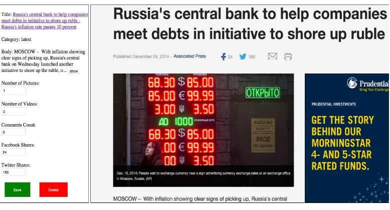
1 An example of what the user sees when browsing foxnews.com . . . 2

2 An example for a regression model line fit through explanatory variable points . . . 7

3 An example of the provided popularity metrics with each story. This particular story had 27 Facebook shares, 80 Twitter shares/tweets, and 86 comments . . . 16

4 The complete crawling process used to collect the stories and their popularity metrics . . . 17

5 A story example of the PHP portal created to manually review all the stories in the dataset . . . 18

6 An example of the text cleaning process . . . 19

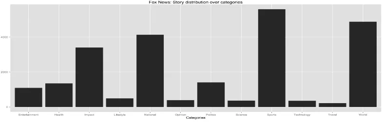
7 The Fox News dataset distribution over categories . . . 20

8 The Huffington Post dataset distribution over categories . . . 21

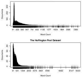
9 Word count per story for both datasets . . . 21

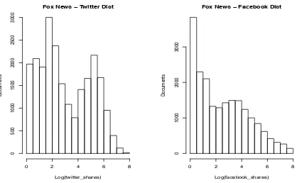
10 The distribution of popularity for Fox News dataset . . . 22

11 The distribution of popularity for The Huffington Post dataset . . . 22

12 The amount of attention (number of Twitter shares) received per story on day1, day2, and day3 for the Fox News dataset . . . 23

13 Linear regression behaviour with di↵erent K values for the Fox News dataset . . . 27

14 Linear regression behaviour with di↵erent K values for the Huffi n-gton Post dataset . . . 27

15 Kendall rank correlation coefficient performance with di↵erent K values for the Fox News dataset . . . 29

(8)

List of Tables

1 An example of the matrix generated by TF-IDF . . . 4

2 An example of a regression model data points . . . 7

3 Classification model performance with di↵erent K values for the

Fox News dataset . . . 30

4 Classification model performance with di↵erent K values for the

Huffington Post dataset . . . 31

5 A summary of the best results found for the regression, ranking,

and classification models . . . 32

6 A comparison between the RMSE of the original content matrix

and the summarized version produced by our approach . . . 32

7 Model performance on the Fox News dataset when predicting for

Twitter shares . . . 33

(9)

1

Introduction

1.1

Overview

The news domain attracts a significant amount of users’ attention. Both

tra-ditional newspapers (e.g. The New York Times) and non-traditional electronic

news websites (e.g. Engadget) compete to build the biggest possible user base.

To measure their success, news providers track the number of views, comments,

and/or shares on social media for each of their articles/blogs. Using those

met-rics, they observed that out of the large number of published articles/blogs, only a

small percentage receives serious user attention. The ability to predict that small

percentage is crucial for the news business and a key factor for the success of

one news provider over the other as popularity prediction can help in forecasting

trends, planning for advertisement campaigns, and estimating future profit/costs.

In general, accurate popularity prediction can lead to improvements in: (1)

advertisement planning, (2) profit/cost estimation, (3) recommender systems

per-formance, as users can be directed to the interesting/popular part of the data,

(4) search engines design and implementation, as items with higher predicted

popularity can be ranked higher than the items with lower predicted popularity,

(5) published material, as the interest and preferences of the majority of users

is understood better, and (6) system administration, as it can help with caching

strategies, traffic management, and possible bottleneck identification.

The complexity of the problem is far greater than it sounds as too many factors

play a role in explaining the attention of users for specific items. Nonetheless, we

could break those factors into extrinsic factors (unrelated to the characteristics of

the item, e.g. a recommendation from a friend) and intrinsic factors (related to the

item, e.g. the title of a video). The extrinsic factors have been covered in various

previous studies (Lerman & Hogg, 2010; He, Gao, Kan, Liu, & Sugiyama, 2014;

Kim, Kim, & Cho, 2012; Lerman & Hogg, 2012; J. G. Lee, Moon, & Salamatian,

(10)

[image:10.595.210.424.71.212.2]

Figure 1: An example of what the user sees when browsing foxnews.com

received that much attention. This lack of attention is due to the complexity in

capturing those intrinsic factors, and to the notion that building models around

the intrinsic factors (e.g. based on the text of news stories), may lead to a solution

that is not easily extended to other data types such as images or videos— which

might be considered an issue for researchers aiming for a general solution. In this

thesis, we focused on building a model that uses the intrinsic factors of a news

story to explain its popularity with less focus on building a general solution.

1.2

Proposed Approach

We will investigate the use of content in popularity prediction. We believe that

the content of a story matters in determining whether it will be popular or not.

The basic intuition behind our approach is that when most users browse their

favorite news source (e.g. Fox News), they only see the story’s title and the media

(images/videos) used with the story as seen on Figure 1. Next, they evaluate

whether they find the topic of the story (inferred from the title) or the media used

with the story, interesting or not, and based on that, they decide whether to read

or skip the story. Thus, we can assume that most users have a list of topics that

they find interesting, and that they use that list to find their next story to read.

Since each news source usually has a large base of the same loyal readers, we can

assume that a set of latent topics exist and may be unique to that news source,

(11)

and their estimated audience, we can build a rough estimation of how popular

that topic will be the next time around. Moreover, to capture the possible user’s

interest in the media used in the story (e.g. set of images or videos), we will

keep track of how many images and/or videos exist in each story. Compared with

existing methods, this is a much better approach for the news domain as we can

make predictions even before an item is released to the public.

We will approach the problem using regression, ranking, and classification

mod-els. Approaching the problem using a regression model means that we will try to

predict the exact number of attention (e.g. comments/views/shares). Whereas,

approaching it using a ranking model, means that we will try to predict the

rank-ing/order of stories by the amount of attention they will receive from highest to

lowest. Finally, in the classification model, instead of predicting a continuous

value, we will try to classify whether a story will be popular or not.

1.3

Thesis Organization (Outline)

In the remainder of this thesis, we will first cover some necessary background

information in section 2 that the reader should know to fully comprehend the

presented work. In section 3, we discuss the previous research done to solve the

problem of popularity prediction in sect. In section 4 we discuss how we gathered

the data needed for this research, and explain all the cleaning process and any

data transformations we did on the dataset, and end this section with an overall

analysis of the dataset. Finally, we discuss our experiment and results in sections

(12)

Terms News Articles (Documents)

iPhone 6 released! Android vs. iOS 2014 smartwatch list

Apple 0.8 0.5 0.3

Google 0.0 0.5 0.2

iPhone 0.9 0.2 0.0

Android 0.0 0.8 0.2

iOS 0.2 0.9 0.3

[image:12.595.127.509.71.189.2]

App Store 0.0 0.7 0.0

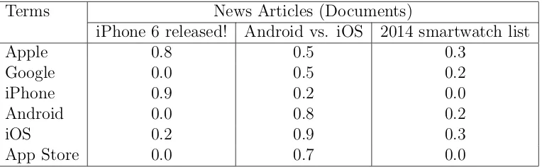
Table 1: An example of the matrix generated by TF-IDF

2

Background

2.1

Term Frequency - Inverse Document Frequency

(TF-IDF)

This is one of the most popular algorithms in the field of information retrieval. It

is mainly used to find the most important words that describe the content of a

document. Given a set of documents, TF-IDF will output a document-term matrix

with values that represent the weight (i.e. importance) of wordi in document j.

An example of what TF-IDF would output given a set of articles about

tech-nology can be seen in Table 1. The numbers represent the TF-IDF weight

(impor-tance score) of term i (e.g. Apple) to article j (e.g. iPhone 6 released). As seen

in Table 1, such a technique can help tremendously in understanding the content

of documents— or articles in our case.

As explained by (Je↵rey David Ullman, Anand Rajaraman, 2015), TF-IDF

finds the words that describe a document based on the observation that important

words that describe the documents are the least frequent words; whereas, the

most frequent words carry the least significance in explaining the content of the

document. This observation might feel a bit counter-intuitive but it has been

proven that the most frequent words are actually stop words that do not carry

(13)

mentioned observation, TF-IDF was introduced with following equations:

T Fi,j =

fi,j

maxk(fk,j)

(1)

IDFi =log(

N ni

) (2)

Wi,j =T Fi,j ⇥IDFi (3)

The first equation (1) captures theterm frequency TFij (i.e. number of

occur-rences) of term i in article j and divides it by the maximum frequency found for

term i among all the articles in the corpus. For example, if we were looking at

articlej (e.g. iPhone 6 released) where the termi (e.g. Apple) occurred two times

and we know that the maximum occurrence of the same term i was nine times at

another article k in the corpus, then the TFij value for the term i and article j is

2/9.

The second equation (2) uses the inverse document frequency IDFi to properly

scale down/up the value of TFij through dividing the total number of documents

by the number of documents that mentions term i in the corpus. For example,

if we had a total of three articles in our corpus and the term i (e.g. Google) has

been mentioned in two documents out of the three, then the IDFi for term i is

log(3

2).

The third equation (3) is used to calculate the final weight score of TF-IDF

for term i and article j by simply multiplying the values from the first and second

equations.

It is important to point out that, for simplicity reasons, we are not explaining

that there’s a need for additional text processing before using TF-IDF such as word

stemming. However, readers should be aware that all the required text processing

(14)

2.2

Non-negative Matrix Factorization (NMF)

In recent years, non-negative matrix factorization (NMF) has become well-known

in the information retrieval field. NMF is used to find two non-negative matrices

whose product can approximate the original matrix; thus, resulting in a smaller

compressed version (D. D. Lee & Seung, 1999). It was used in a number of

computer science fields including computer vision, pattern recognition, document

clustering, and recommender systems. The technique has shown tremendous

suc-cess especially after it won the Netflix challenge (Koren, Bell, & Volinsky, 2009) by

greatly improving their movie recommendation system. In a movie

recommenda-tion setting, the system usually maintains data about users and the ratings given

for items by each user in the form of a matrix. However, that matrix is usually

very sparse as users rarely rate items, which is where NMF comes in. NMF tries

to approximate that matrix as an inner product of two low-rank matrices, as seen

in equation (4), in order to capture the latent feature space that explains why user

u gave that specific rating to itemi.

Vu,i ⇡Wu,k⇥Hk,i (4)

The W matrix shows us the level of influence that the factors in the latent space

have on the taste of useru; whereas, theH matrix would shows us the importance

of the latent space factors in rating itemi. Then, given those two matrices,we can

approximate values for the empty slots in the original matrix. This technique won

the Netflix challenge, and since then has been used in many domains, but to the

best of our knowledge, has never been used in the popularity prediction domain.

2.3

Linear and Logistic Regression

Regression is a statistical approach for modeling the relationship between a

re-sponse variable y, and one or more explanatory variables (i.e. features). The

(15)

X (Model Feature) Y (Model Response)

0.5 0.2

1 1.5

1.5 2.5

2 1.8

[image:15.595.201.432.71.159.2]

3 2

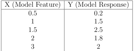
Table 2: An example of a regression model data points

fit throughout the feature points that would explain their relationship with the

response variable. For example, based on the data in Table 2, a typical scenario

would be to predict the value of the response variable y based on the value of the

explanatory variablex. As seen in Table 2, we know the value ofy whenx is_{0.5,

1, 1.5, 2, 3_}, and using a regression model we can predict the value ofy for other

[image:15.595.204.428.405.627.2]

values of x (e.g. when X is 4) by fitting a line through the data points as seen in

Figure 2. For instance, using our fitted line, we predict that y will be 4 whenx is

4.

x axis y axis

0 1 2 3 4

Figure 2: An example for a regression model line fit through explanatory variable points

In general, when we use a simple regression model, we try to fit the best line

between the given points that would minimize the distance measured vertically

between the points and the model line. Next, we use the fitted line to make

(16)

value of the response variable y; whereas, in logistic regression, the fitted line is

used to break the observations into two classes (e.g. popular/not-popular), so for

example, we could label all points that fall above the fitted line as class A (e.g.

popular) and all points that fall below the fitted line as classB (e.g. not-popular).

In our work, we use linear regression to predict the exact number of shares

(i.e. the response variable) using the hidden topics found in the content (i.e.

explanatory variables). Moreover, we use logistic regression to classify stories as

either ”popular” or ”not-popular” using the same set of explanatory variables.

2.4

Performance Measures

2.4.1 Root Mean Square Error (RMSE)

To measure the performance of a regression model, a number of performance

metrics can be used; among those is Root Mean Square Error or RMSE. The

RMSE is used to measure the di↵erence between the true and predicted values

using the following formula:

r

(1

n)⇤

X

(predicted actual)2 ₍₅₎

where n is the number of observations in the dataset, predicted is a vector

repre-senting the predicted values, and actual is a vector representing the true values.

2.4.2 Kendall Rank Correlation Coefficient

The Kendall Correlation Coefficient is a statistical test that measures the similarity

between two orderings through the following formula:

(nc) (nd)

1

2n(n 1)

(6)

where nc is the number of concordant pairs, nd is the number of discordant

pairs, and n is the number of observations. The Kendall Correlation Coefficient

(17)

two rankings, and -1 means that the two rankings are opposites. For instance,

if vector-1 is _{1,2,3,4_}, vector-2 is _{4,3,2,1_}, and vector-3 is _{1,2,3,4_}, and we

want to measure the correlation between vector-1 and the other two vectors using

Kendall Correlation Coefficient. Then, using the given formula, we will find that

the correlation between vector-1 and vector-2 would be -1; whereas, the correlation

between vector-1 and vector-3 would be +1. Thus, it gave us a good indication of

the similarity in the ordering between the two vectors.

2.4.3 Accuracy, Precision, Recall, and F-score

Unlike the previous models, to measure the performance of a classification model,

multiple metrics are needed as follows:

First, there is the accuracy metric that measures the overall performance of

the classification model. It uses the following formula:

Accuracy= T P +T N

T P +F P +F N +T N (7)

where TP is the number of correct classifications for the positive class, TN is

the number of correct classifications for the negative class, FP is the number of

incorrect classifications for the positive class, and FN is the number of incorrect

classifications for the negative class. Simply put, it divides the number of correct

classifications by the total number of classifications — both correct and incorrect

classifications.

Second, there is the precision metric that measures the accuracy of the positive

class predictions, specifically, out of all the positive class predictions, how many

were correct? This intuition is captured by the following formula:

P recision= T P

T P +F P (8)

Third, there is the recall metric that measures how accurate is our classification

(18)

we accurately classify as positive? This intuition is captured by the following

formula:

Recall = T P

T P +F N (9)

Finally, there is the f-score metric which is a measure that acts as a weighted

average of precision and recall. This means that the f-score measure is a mean for

us to determine how well our model is doing on both precision and recall as seen

in its formula:

f-score= 2⇤P recision⇤Recall

P recision+Recall (10)

It’s important to note in here that the reason why we used Precision and Recall

is that those measures focus on the positive class (i.e. popular class) which is our

main focus. Remember that the goal of popularity prediction is to find the popular

fraction of stories using those measures, and thus we can determine how well we’re

(19)

3

Related Work

Szabo and Huberman were the first to notice that there is a linear relationship

be-tween the log-transformed long-term popularity of a given item and its early view

patterns (Szabo & Huberman, 2010). Based on that observation, they proposed

a linear regression model on a logarithmic scale that predicts the total number

of views for a future date using the number of views from an earlier date. They

tested their model using YouTube videos and Digg stories— a popular user-driven

news website where users post links to news articles and collectively vote them

up or down. They were able to estimate the popularity with only 10% error rate

using a simple linear model.

A follow up study on that approach suggested that not all dates are equally

important in terms of the attention they get; thus, using di↵erent weights for

di↵erent days would improve the overall model. That simple change resulted in

up to 20% improvement in accuracy (Pinto, Almeida, & Gon¸calves, 2013).

A similar study investigated the ability to predict the number of comments for

a future date based on the number of comments from an earlier date. They tried

three di↵erent techniques: a simple linear model, a linear model on a logarithmic

scale that was suggested by Szabo and Huberman , and a constant scaling model.

Surprisingly, their results showed that the simple linear model outperformed the

other two models (Tatar, Antoniadis, de Amorim, & Fdida, 2012).

The previously mentioned approaches are simple and accurate but they rely

on the early view patterns which is a problem when it comes to news articles as

they have a short life span. It would be much more convenient if the popularity

was predicted even before the public sees the articles.

Another study on popularity prediction argued that merely using the number

of comments to predict popularity is not enough. Thus, they argued that using

social influence, represented by the number of friends a user has, would result

in a better ranking accuracy for popularity prediction. To test their claim, they

(20)

results that prove how considering other features such as social influence can help

in popularity prediction (He et al., 2014).

Moreover, Lerman and Hogg studied predicting the popularity of news on

Digg by considering the website layout and by modeling user voting behavior

explicitly as a stochastic model. They found that the two most important factors

for popularity prediction are the quality of the story and the social influence of

users in Digg. They built a model that evaluates how interesting a story is (story’s

quality) based on the early user reactions to it through the voting system. Then,

based on how interesting the story is and how connected the submitter is (social

influence), they predicted the final voting count that a story will receive (Lerman

& Hogg, 2010, 2012).

Also an interesting model based approach was suggested in a di↵erent study

where they worked on predicting the number of votes based on exploiting users

voting behavior. They argued that users are either mavericks or conformers where

mavericks are users that vote based on the opinion of the majority, and conformers

are users who vote against the opinion of the majority, and that when a user votes,

one of those two personalities prevail. Based on that, they built a model that

incorporated both the suggested user personalities and the early number of votes

to predict the future number of votes for a given item (Yin, Luo, Wang, & Lee,

2012).

With a di↵erent focus, a study characterized the popularity patterns of YouTube

videos and demonstrated the impact of referrers (i.e. source of incoming links)

on popularity prediction (Figueiredo, Benevenuto, & Almeida, 2011; Figueiredo,

2013).

Using a di↵erent approach, another study predicted the probability that a

thread in a discussion forum will remain popular in the future using a biology

inspired survival analysis technique. They identified risk factors such as the

to-tal number of comments and the time between the thread creation and its first

(21)

input, they output a metric for popularity that shows the probability of whether

a thread will remain popular in the future or not (J. G. Lee et al., 2010).

It’s worth mentioning that some work has approached this problem as a

clas-sification problem as well where they predict whether an item will be popular or

not (Wu, Timmers, Vleeschauwer, & Leekwijck, 2010; Bandari, Asur, &

Huber-man, 2012; Kim et al., 2012). An example of such work is where the authors

used reservoir computing which is a special type of neural networks to predict the

popularity of items based on early popularity data (Wu et al., 2010). However,

their model was complex and could not outperform the simpler linear regression

model suggested by Szabo and Huberman. Also, another study focused on

ana-lyzing the popularity of news blogs (Kim et al., 2012). They used SVM, baseline,

and similar matching to classify blogs. Their results show that they were able to

predict whether an article will be popular or not after eight hours from submission

with an overall accuracy of 70% .

The only attempt, to the best of our knowledge, which tries to predict the

popularity of items without incorporating early popularity metrics was in 2012,

where researchers attempted to predict the popularity of news articles based on

factors related to the content (Bandari et al., 2012). They considered the

fol-lowing factors: the news source, the article’s category, the article’s author, the

subjectivity of the language in the article, and number of named entities in the

article. Their results show that they were able to predict ranges of popularity

(classification) with accuracy up to 84% without considering other factors that

have been extensively used in previous research such as early view/comment/vote

data or social influence. They evaluated their work on a one-week worth of news

dataset from 1350 di↵erent news source that they collected using a news

aggrega-tor API service. We align ourselves with this kind of work. However, they only

used features extracted from the content, not the content itself.

This research di↵ers from this work and all the previous research in that it

(22)

specifically the news content. Also, the approach suggested in this research makes

predictions even before an item is released as it does not rely on data from the

(23)

4

Dataset

4.1

Data Collection

We used Alexa, which is an Amazon.com company for web analytics, to find two

popular news sources to crawl for stories. Based on Alexa, The Huffington Post

and Fox News are among the top-20 most visited news websites in the United

States and among the most famous around the world. For that reason, we started

crawling the two websites for stories on December 24th, 2014 and stopped on

March 15th, 2015 which gave us approximately three months’ worth of data.

PHP was used to read all the RSS feeds provided by both websites. Fox News

had 12 RSS feeds broken down by di↵erent categories; whereas, The Huffington

Post had 20 RSS feeds, also broken down by categories. It was a straight XML

document read for all the RSS feeds. The RSS provided the title, category, and the

link to each story. Next, the HTML structure of each website was analyzed and

four patterns were found in common between the stories of Fox News, and three

patterns forThe Huffington Post. Using those patterns, all the links were crawled

to get the complete text for each story. All the data was stored in a MySQL

database to allow for complex queries — if needed. An hourly job was scheduled

to read the RSS of both websites for new stories through the whole period, and a

separate job was scheduled every 30 seconds to crawl the full body for the stories

using the links stored in the MySQL database.

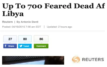
Next, to get the popularity metrics (number of comments/Facebook and

Twit-ter shares), found with every story as seen in Figure 3, a separate script was needed

as those metrics were populated through JavaScript after the page loads, and since

PHP only retrieves the static HTML files prior to any JavaScript manipulation,

it wasn’t possible to retrieve those metrics with it. Thus, a combination of our

JavaScript code, CasperJS1_{, and PhantomJS}2 _{was used to crawl the two websites}

for popularity metrics. The script used stimulates a browser request, and then it

1_{http://casperjs.org/}

(24)

[image:24.595.228.409.71.184.2]

Figure 3: An example of the provided popularity metrics with each story. This particular story had 27 Facebook shares, 80 Twitter shares/tweets, and 86 com-ments

waits 10 seconds to allow for any existing JavaScript to execute and manipulate

the HTML, then it pulls the final HTML code which includes the actual

popu-larity metrics. A separate job was scheduled for each website to run the script

every second and pull the popularity metrics for the stories stored in the MySQL

database based on their publication day.

We started collecting the popularity metrics for each story on daily basis for a

period of seven days starting from the publication day. Previous research (Szabo

& Huberman, 2010) shows that by the end of the first day, users lose interest in

Digg news stories. It is worth mentioning that we also collected the category each

story falls under and the number of images/videos contained in the body of each

story.

To run the previously mentioned jobs, two Amazon Elastic Compute Cloud

or EC2 machines were configured and used throughout the crawling period. The

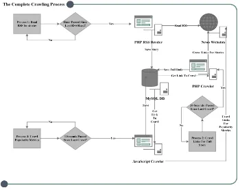
whole crawling process is summarized in Figure 4.

4.2

Data Cleaning

Since the dataset was collected through an automated process that may fail from

time to time, it was necessary to manually check the stories in the dataset to

confirm its consistency and integrity. Thus, after the data collection was complete,

a simple PHP portal was created, as seen in Figure 5, which pulls stories from the

(25)

[image:25.595.142.492.71.349.2]

Figure 4: The complete crawling process used to collect the stories and their popularity metrics

story on the right side (using the story’s link), and then a manual comparison

between the two was made. If a story was missing its body, then it would be

discarded. If a story had the wrong number of images, number of videos, number

of final Twitter shares, or number of final Facebook shares, it would be updated.

After that process was complete, 20% of the stories in the dataset were removed,

mostly due to broken links or links pointing to external websites that the crawler

wasn’t familiar with, and thus couldn’t crawl.

4.3

Data Preparation

First, we combined the title and body of each story, and then we removed

whites-pace, numbers, Punctuation, HTML tags, and stop words. Next, we enforced

lower case letters and applied word-stemming on the whole body of text. Figure 6

shows an example of a before and after for an example text. It’s worth mentioning

that we found the Text Mining Package to be a great help in accomplishing this

(26)

[image:26.595.122.511.68.278.2]

Figure 5: A story example of the PHP portal created to manually review all the stories in the dataset

Before Processing:

Graduate study in a computing discipline that only focuses on traditional

com-puting approaches is not flexible enough to meet the needs of the real world.

New hardware and software tools are continually introduced into the market.

IT professionals must have a specific area of expertise as well as be adaptable

and ready to tackle to the next new thing-or just as often, retrofit available

technologies to help their users adapt to the latest trends. The MS in

informa-tion sciences and technologies provides an opportunity for in-depth study to

prepare for today”s high-demand computing careers. Companies are

drown-ing in data-structured, semi-structured, and unstructured. Big data is not just

high transaction volumes; it is also data in various formats, with high velocity

change, and increasing complexity. Information is gleaned from unstructured

sources-such as Web traffic or social networks-as well as traditional ones; and

information delivery must be immediate and on demand.

After Processing:

graduat studi comput disciplin focus tradit comput approach flexibl enough

(27)

pro-fession must specif area expertis well adapt readi tackl next new thingor just

often retrofit avail technolog help user adapt latest trend ms inform scienc

technolog provid opportun indepth studi prepar today highdemand comput

career compani drown datastructur semistructur unstructur big data just high

transact volum also data various format high veloc chang increas complex

in-form glean unstructur sourcessuch web traffic social networksa well tradit one

inform deliveri must immedi demand

Figure 6: An example of the text cleaning process

Second, we removed very short stories. Since we are exploring the possible

use of content to predict popularity, we must have stories with enough content

(words). Thus, we decided to remove all stories with fewer than 40 words.

Third, we removed outliers from the dataset. We used the Extreme Studentized

Deviate test or ESD which uses the following formula to find the outliers in the

dataset:

[mean (t_⇤SD), mean+ (t_⇤SD)] (11)

where SD is Standard Deviation and t is a threshold value that we determine

based on our data. As seen by the formula, the ESD test declares any point

more than t standard deviations from the mean to be an outlier value. We found

three to be a good value for the t threshold. We used ESD on both Twitter and

Facebook shares and kept only the stories that fall between the upper and lower

bounds.

Fourth, we generated two text files, one for each news source, with the complete

dataset. The text files contain the following for each story: 1) story id, 2) story

text, 3) story category, 4) story image count, 5) story video count, 6) story Twitter

(28)

[image:28.595.121.513.76.202.2]

Figure 7: The Fox News dataset distribution over categories

4.4

Data Exploration and Analysis

This section will explore the content of the dataset:

4.4.1 Dataset size

The initial Fox News dataset had approximately 27,000 stories. However, after we

cleaned and prepared the dataset for analysis, the Fox News dataset size dropped

to 23,363 stories. As for the Huffington Post dataset, it had approximately 29,000

stories and was cut down to 23,583 stories after cleaning and preparing the dataset.

4.4.2 Story distribution over categories

The Fox News dataset has 12 categories/sections for news stories. The distribution

of the stories in the dataset can be seen in Figure 7. We can see that most stories

are from the sports, world (i.e. international news), and national (i.e. local news)

categories/sections.

As for the Huffington Post dataset, there’s a larger variety of categories/sections.

The dataset has 20 categories/sections, as seen in Figure 8, with a the majority

of stories being from the blogs, world (i.e. international news), and entertainment

category/section.

4.4.3 Average number of words

The Fox News dataset word count distribution can be seen in Figure 9 which

(29)

[image:29.595.121.514.76.200.2]

Figure 8: The Huffington Post dataset distribution over categories

0

100

200

300

Fox News Dataset

Word Count

Documents

41 203 385 567 751 933 1138 1377 1624 1864 2096 2383

0

20

40

60

80

The Huffington Post Dataset

Word Count

Documents

41 641 1394 2233 3073 3901 4786 6653 8127 9033

Figure 9: Word count per story for both datasets

90 and 500 words. As seen in Figure 9, the Huffingon Post dataset average number

of words is 273 word per story which is higher than the Fox News dataset but it

had a very similar distribution with word count falling between 100 and 700 words

for most of the dataset.

4.4.4 Popularity Distribution

The metrics we are using to measure popularity are Twitter and Facebook shares.

[image:29.595.168.456.249.529.2]

(30)

Fox News − Twitter Dist

Log(twitter_shares)

Documents

0 2 4 6 8

0 500 1000 1500 2000 2500 3000

Fox News − Facebook Dist

Log(facebook_shares)

Documents

0 2 4 6 8

0

1000

2000

[image:30.595.203.412.71.200.2]

3000

Figure 10: The distribution of popularity for Fox News dataset

The Huffington Post − Twitter Dist

Log(twitter_shares)

Documents

0 1 2 3 4 5 6 7

0 500 1000 1500 2000 2500

The Huffington Post − Facebook Dist

Log(facebook_shares)

Documents

0 2 4 6 8 10

0 500 1000 1500 2000 2500

Figure 11: The distribution of popularity for The Huffington Post dataset

just merely clicking or viewing the story as it requires the user to interact with the

story by clicking on the share button. The distribution of those two metrics on a

logarithmic scale can be seen in Figure 10 and 11 for the Fox News and Huffington

Post datasets respectively.

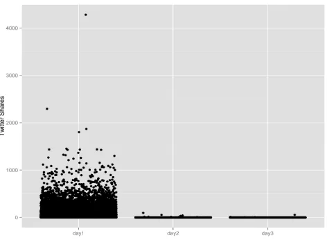
4.4.5 Attention on 1st day vs. following days

For both the Fox News dataset and Huffinton Post dataset, we found that news

stories do received 90%-100% of all the attention they will ever get during the first

day as seen in Figure 12 — which shows the number of Twitter shares received

by Fox New stories on the first, second, and third day. This proves our point that

unlike YouTube videos where a video may still be relevant and attracts attention

for years to come, news stories have a very short life span, a few hours in some

cases, which shows how important it is to predict the popularity even before the

[image:30.595.203.412.238.365.2]

(31)

[image:31.595.198.434.74.247.2]

Figure 12: The amount of attention (number of Twitter shares) received per story on day1, day2, and day3 for the Fox News dataset

5

Experiment

5.1

Approach Summary

We summarize our suggested approach here and give further details in the following

section:

• We built a matrix that represents the content of our dataset using term

frequency-inverse document frequency (TF-IDF). The TF-IDF matrix was

built using the text of the stories (both title and body). This can be

gener-alized to any domain as long as the content can be represented as a matrix.

• We applied non-negative matrix factorization (NMF) to the TF-IDF matrix

to find the latent topics that help in explaining the user’s interest in each

story. Moreover, NMF helped in summarizing the original term-based matrix

which gave us a smaller matrix that is much more computationally efficient

to use for model training and prediction. In our case, it resulted in an up to

90% smaller matrix and gave us better accuracy than the original term-based

matrix.

• We integrated the other features that we extracted from the content to the

(32)

story’s category, the number of images, and number of videos found in the

body of each story.

• We used the final matrix in our regression, ranking, and classification models

to predict the popularity of news stories.

5.2

Constructing the Terms Dictionary

When we built the terms dictionary, which is the first step to build the TF-IDF

matrix, we found that it had a large number of terms for both datasets due to

infrequent terms (terms that occur in only a few stories). For that reason, we had

to pick a threshold that would allow us to drop the infrequent terms and lower

the final TF-IDF matrix size. We picked two thresholds, a low one (20), and a

high one (80). This means that for the low threshold (20), we dropped all the

terms that occurred in fewer than 20 stories; whereas, for the high threshold we

dropped all the terms that occurred in fewer than 80 stories. Next, we compared

the performance of both on predicting popularity using a regression model, and

compared the results between the two. We found the error rate di↵erence to be

minimal. This may be due to the fact that the less frequent a term is, the less

useful it is to help in other stories in the dataset. As a result, we used the matrix

with the high threshold (80) in our model evaluation as it is a smaller matrix,

which makes it computationally more efficient. After applying our threshold, the

Fox News dataset dictionary had 4822 terms; while, the Huffington Post dataset

dictionary had 6107 terms.

5.3

Building the TF-IDF Matrix

The TF-IDF matrixAhas rows that represent stories and columns that represent

terms (from the dataset dictionary), where element Ai,j represents the TF-IDF

weight of term j in story i. Based on that, the A matrix for the Fox New dataset

(33)

dataset had 23,583 rows and 6107 columns.

5.4

Discovering Hidden Topics using NMF

To explain how we used NMF to discover the hidden topics, let’s assume that there

arem articles andn distinct terms. We use a matrixA₂Rm₊⇥n to denote the

TF-IDF matrix, whereAij represents the TF-IDF weight of word j in article i. Note

that entries in the TF-IDF matrix all take non-negative real values. In this regard,

thei-th row ofArepresents articleiwhile thej-th column ofArepresents termj.

NMF computes two low-rank matrices G2Rn⇥K

+ and H2RK+⇥m to approximate

the original TF-IDF matrix A, i.e., A⇡GH0. More specifically,

aj ⇡

K

X

k=1

Gjkhk (12)

where aj is the j-th column vector in A, representing term j, and hk is the k-th

column of H. Eq. 12 shows that each term vector aj is approximated by a linear

combination of the column vectors in H weighted by the components of G. In

practice, we have K ⌧m and K ⌧n. Hence, H can be regarded as a new basis

that contains a lower number of basis vectors than A. These new basis vectors

capture the latent topics that characterize the underlying content of the articles.

Consequently, G is the new representation of the articles using the latent topics.

It can also be regarded as a projection of A onto the latent topic space H.

To apply NMF, we need to choose a factorization rankK, so we experimented

with di↵erent values forK until we found the value that gave us the best accuracy

for each of the models. In our experiment, we built seven matrices, each with a

di↵erent K value as follows: 200, 400, 500, 1000, 1500, 2000, and 3000. Next,

we used those matrices with all three models and documented the results in the

(34)

5.5

Integrating Heterogeneous Features

The hidden topics discovered using NMF are expected to provide a good and

compact approximation of the TF-IDF matrix, which captures the content of

the news articles. The remaining challenge is how to exploit the new content

representation to achieve popularity prediction. Recall that entries Gjk’s for k 2

[1, K] essentially denote the importance or weight of each of theK topics in article

j. Therefore, if we treat topics as features to describe the content of articlej,Gjk’s

can be used as the feature values in a popularity prediction model. Meanwhile,

as part of our collected data, the numbers of Twitter and Facebook shares show

people’s interest in an article, which provides a natural indicator of its popularity.

Therefore, we choose these numbers as the response of our popularity prediction

model.

Besides the hidden topics, some other features embedded in a news article may

also be useful for popularity prediction. For example, we also included the story’s

category as a feature in our model based on our observation that the category of

a story plays a big role in determining its future popularity. Moreover, we noticed

that there is a fraction of stories where the attention is not on the textual part

of the story but the media used in the story whether that be a set of images or

videos. Thus, we decided to use the number of images and the number of videos

used within a story as features in our model as well.

5.6

The Regression Prediction Model

We propose to exploit a multivariate regression model to integrate these

heteroge-neous set of features for popularity prediction. We trained the model with 10-fold

cross validation. The in-sample (training) and out-of-sample (testing) errors can

be seen in Figure 13 for the Fox News dataset, and in Figure 14 for the Huffington

Post dataset— when predicting for both Twitter and Facebook shares. We used

Root Mean Square Error (RMSE) to evaluate the linear regression model.

(35)

200 500 1500 3000 1.15 1.20 1.25 1.30 1.35

Twitter Training Error

K−value (Factorization Rank)

RMSE

200 500 1500 3000

0.675

0.680

0.685

0.690

0.695

Twitter Testing Error

RMSE

200 500 1500 3000

1.25

1.30

1.35

1.40

1.45

Facebook Training Error

RMSE

200 500 1500 3000

0.735

0.745

0.755

Facebook Testing Error

[image:35.595.185.422.101.343.2]

RMSE

Figure 13: Linear regression behaviour with di↵erent K values for the Fox News

dataset

200 500 1500 3000

1.70

1.75

1.80

1.85

Twitter Training Error

RMSE

200 500 1500 3000

0.95

0.97

0.99

1.01

Twitter Testing Error

RMSE

200 500 1500 3000

1.45

1.50

1.55

1.60

Facebook Training Error

RMSE

200 500 1500 3000

0.83

0.84

0.85

0.86

0.87

Facebook Testing Error

RMSE

Figure 14: Linear regression behaviour with di↵erentK values for the Huffington

[image:35.595.185.423.455.697.2]

(36)

value, we get a lower in-sample (training) error. This held true for both datasets

and when predicting for both Twitter and Facebook shares.

For the Fox News dataset, we observed that when predicting for Twitter shares,

we got a U-shape where K is 1000, and an almost U-shape with Facebook where

K is 2000. Thus, we picked a K value of 1000 when predicting for Twitter and a

K value of 2000 when predicting for Facebook.

For the Huffington Post dataset, we observed that when predicting for twitter

shares, the simpler model gave the best out-of-sample (testing) error; whereas,

when predicting for Facebook, we get our U-shape pattern again where K is 500.

Thus, we picked a K value of 500 when predicting for Twitter and Facebook

shares.

5.7

The Ranking Prediction Model

We used the predictions of the linear regression model to solve this as a ranking

problem. For each factorization rankK, we sorted vector-1 which has the correct

ordering of stories by the number of shares from highest to lowest, and vector-2

which has our predicted values of shares sorted from highest to lowest as well,

and we compared the two vectors. To compare the two vectors, we used Kendall

rank correlation coefficient, and we demonstrated the in-sample (training) and

out-of-sample (testing) results in Figure 15 and in Figure 16.

In general, we noticed that the ranking correlation increased and decreased

based on how well the linear regression model performed. Thus, for the in-sample

(training) results, we found that the correlation increases as we increased the

factorization rank K; moreover, the out-of-sample (testing) results for the Fox

News dataset, acted similarly to the linear model in that the highest correlation

was whenK is 1000, when predicting for Twitter shares, and 2000 when predicting

for Facebook shares. The values we picked for K when training the linear model,

are the best ones for the ranking model as well. As for the Huffington Post

(37)

200 500 1500 3000 0.54 0.56 0.58 0.60 0.62

Twitter In−sample

K

endall r

ank correlation

200 500 1500 3000

0.542

0.546

0.550

0.554

Twitter Out−of−sample

K

endall r

ank correlation

200 500 1500 3000

0.50

0.52

0.54

0.56

0.58

Facebook In−sample

K

endall r

ank correlation

200 500 1500 3000

0.495

0.500

0.505

0.510

Facebook Out−of−sample

K

endall r

[image:37.595.185.422.72.312.2]

ank correlation

Figure 15: Kendall rank correlation coefficient performance with di↵erentK values

for the Fox News dataset

both Facebook and Twitter shares.

5.8

The Classification Prediction Model

We chose to break the dataset up into 25% popular stories and 75% unpopular

stories to make it more realistic as popular stories in real-world data represent

only a fraction of the available content. Thus, we labeled the top 25% most shared

stories in both datasets as popular, and labeled all other stories as not-popular.

We used logistic regression for classification and we experimented with di↵erent

values for the factorization rank K in here as well. To measure the performance

we used common classification measures: accuracy, precision, recall, and f-score.

The in-sample and out-of-sample results can be seen on table 3 for the Fox News

dataset, and table 4 for the Huffington Post dataset.

In general, we observed that for the in-sample results (training), we got a

similar pattern to that of the other models where we get a higher accuracy and

f-score as we increase the factorization rank. This is seen for both datasets.

(38)

200 500 1500 3000

0.20

0.25

0.30

Twitter In−sample

K

endall r

ank correlation

200 500 1500 3000

0.140

0.150

0.160

Twitter Out−of−sample

K

endall r

ank correlation

200 500 1500 3000

0.38 0.40 0.42 0.44 0.46 0.48

Facebook In−sample

K

endall r

ank correlation

200 500 1500 3000

0.345

0.355

0.365

Facebook Out−of−sample

K

endall r

[image:38.595.184.423.84.322.2]

ank correlation

Figure 16: Kendall rank correlation coefficient performance with di↵erentK values

for the Huffington Post dataset

Metric Twitter Accuracy (in-sample)

K=200 K=500 K=1000 K=2000

Accuracy 0.7993 0.8195 0.8351 0.8711

Precision 0.6359 0.6785 0.7063 0.7692

Recall 0.4531 0.5221 0.5778 0.6885

F-score 0.5292 0.5901 0.6356 0.7266

Twitter Accuracy (out-of-sample)

Accuracy 0.7902 0.8018 0.8003 0.7998

Precision 0.6104 0.6317 0.6194 0.6054

Recall 0.4329 0.4871 0.5112 0.5611

F-score 0.5065 0.5501 0.5601 0.5824

Facebook Accuracy (in-sample)

Accuracy 0.8018 0.8218 0.8592 0.8774

Precision 0.6367 0.6743 0.7406 0.7773

Recall 0.4613 0.5396 0.6623 0.7065

F-score 0.5350 0.5995 0.6993 0.7402

Facebook Accuracy (out-of-sample)

Accuracy 0.796 0.8082 0.8217 0.8198

Precision 0.6226 0.6431 0.6557 0.6469

Recall 0.4442 0.5039 0.5870 0.5965

F-score 0.5185 0.5650 0.6194 0.6207

Table 3: Classification model performance with di↵erent K values for the Fox

[image:38.595.183.451.395.710.2]

(39)

Metric Twitter Accuracy (in-sample)

K=200 K=500 K=1000 K=2000

Accuracy 0.7556 0.761 0.7729 0.7881

Precision 0.51964 0.56275 0.62173 0.64366

Recall 0.07417 0.12376 0.19491 0.30962

F-score 0.1298 0.2029 0.2968 0.4181

Twitter Accuracy (out-of-sample)

Accuracy 0.7549 0.7504 0.7451 0.7269

Precision 0.5092 0.4690 0.4487 0.3920

Recall 0.07161 0.1173 0.1622 0.2019

F-score 0.1256 0.1877 0.2383 0.2665

Facebook Accuracy (in-sample)

Accuracy 0.7743 0.7855 0.802 0.8235

Precision 0.61051 0.63502 0.6730 0.7123

Recall 0.26402 0.32965 0.4017 0.4907

F-score 0.3686 0.4340 0.5031 0.5811

Facebook Accuracy (out-of-sample)

Accuracy 0.7612 0.7673 0.7633 0.7559

Precision 0.5502 0.5664 0.5422 0.5154

Recall 0.2330 0.2866 0.3274 0.3554

[image:39.595.180.453.69.383.2]

F-score 0.3274 0.3806 0.4083 0.4207

Table 4: Classification model performance with di↵erent K values for the Huffi

n-gton Post dataset

dataset, as seen in Table 3, we get a higher f-score as we increase the value forK

but the overall accuracy starts to drop afterK is 500 when predicting for Twitter

shares, and 1000 when predicting for Facebook shares. The same pattern is seen

for the Huffington Post in Table 4, where the f-score value increases with higher

K value; whereas, the overall accuracy starts to drop after K is 200 for Twitter

(40)

Model Used Fox News Dataset Huffington Post Dataset

Twitter Facebook Twitter Facebook

Regression RMSE 0.6742068 0.7312376 0.9445133 0.824276

Ranking Kendall Correlation 0.5547424 0.5119817 0.1657863 0.3693125

[image:40.595.108.533.74.147.2]

Classification Accuracy 80% 82% 75% 76%

Table 5: A summary of the best results found for the regression, ranking, and classification models

Dataset Original Content Matrix Summarized Content Matrix

Twitter Facebook Twitter Facebook

Fox News 0.761400 1.219993 0.6742068 0.7312376

[image:40.595.110.521.209.270.2]

The Huffington Post 1.123824 1.004408 0.9445133 0.824276

Table 6: A comparison between the RMSE of the original content matrix and the summarized version produced by our approach

6

Results and Discussion

6.1

Results Summary

Table 5 has the best results for the regression, ranking, and classification models

based on the results of the testing sample. Overall, we had better results with the

Fox News dataset than the Huffington Post dataset in all three models. We would

like to highlight the drastic di↵erence done to the size of the original content

ma-trix. For instance, in the regression model, the original term-based content matrix

for Fox News had 4822 columns and was cut down to 1000 columns (20% the

original size) when predicting for Twitter shares, and to 2000 columns (41% the

original size) when predicting for Facebook shares. Also, the original content

ma-trix for Huffington Post had 6107 columns and was cut down to 500 columns (8%

the original size) when predicting for Twitter and Facebook shares. This drastic

size reduction lead to a summarized representation that is much more

computa-tionally efficient for model training and prediction. Moreover, to prove that the

new representation, which uses the latent topics for prediction, performs much

better than the original content matrix, we compared the two using a regression

(41)

Model Used RMSE Kendall Correlation Accuracy

Features-without-content 0.8382228 0.3241783 0.7741

Content-without-features 0.710004 0.5272800 0.7793

[image:41.595.128.506.71.131.2]

Content-with-features 0.6742068 0.5547424 0.7983

Table 7: Model performance on the Fox News dataset when predicting for Twitter shares

6.2

Model Evaluation

To evaluate our model and show the importance of utilizing content when

predict-ing the popularity of items, we compare the followpredict-ing models as we try to predict

the total number of Twitter shares on both dataset:

• Features-without-content model: We only used the category, number of

im-ages, and number of videos as features for this model. We did not incorporate

the content.

• Content-without-features model: We used only the content without any of

the other features.

• Content-with-features model: We used both content and features.

For the comparison done on the Fox News dataset, shown in Table 7, we observe

that the biggest improvement happens when the content is considered. We can

see that the lowest performance happens when considering the features only; then

a jump in performance happens when we consider the content, and then a good

improvement happens when we merge the two which proves that the content can

greatly impact the performance, and when merged with any other features, it can

improve the overall accuracy.

Moreover, we show that it can be combined with other models to improve

their overall accuracy. We used the S-H Model that uses linear regression on a

logarithmic scale proposed by (Szabo & Huberman, 2010) which is considered

the simplest and most accurate model to date. The model uses the early user

(42)

Model Used RMSE

S-H 0.2871537

S-H with-content 0.2810069

[image:42.595.206.423.70.132.2]

S-H with-content-n-features 0.2769502

Table 8: Improving the S-H Model performance by utilizing the content

used the number of Twitter shares received on the first day to predict the final

number of Twitter shares. Note that in the news domain, as previously mentioned,

most stories receive 90% to 100% of the attention they will ever get on the first

day! This means that in reality this model may not be the best model for the news

domain as what matters is the level of attention that the story will get on the first

day and not after. It is unfair to compare our model against the S-H model as we

predict even before an item is released to the public. Thus, we instead prove that

we can improve it by leveraging the content using our suggested approach as seen

in Table 8. The RMSE was already very low when using the S-H model but we

were able to get an even lower value when we included the content, and we got an

(43)

7

Conclusion

In this work, we’ve discussed the short life span nature of news stories, and

ex-plained how it is more efficient to predict the popularity of stories even before they

are released to the public. To tackle this challenge, we have investigated the

abil-ity to use the content of news stories for popularabil-ity prediction. We presented an

approach that uses non-negative matrix factorization to discover the latent topics

that explain the user’s interest in the content of a given story. Then, using these

topics, we estimated the popularity of other stories. To show the e↵ectiveness of

our approach, we evaluated our work on two real-world datasets and showed how

utilizing the content can increase the overall performance whether the goal is to

use a regression, ranking or a classification model. Moreover, we showed how our

approach summarized the term-based matrix, that represents the content, and

reduced its size by up to 90% without losing any prediction accuracy. In contrast,

our summarized version, had higher overall accuracy than the original term-based

matrix. Finally, we proved that the content can be used with other models to

improve their overall performance for popularity prediction. We summarize our

major contributions as follows:

• We suggested a non-negative matrix factorization (NMF) based approach

that utilizes content information to achieve popularity prediction. We used

the popularity of news stories as a motivating example, but the proposed

approach can be applied to other domains where popularity of the items

need to be estimated before the items are released to the public.

• We showed how our approach can summarize the content and produce a

matrix up to 90% smaller than the original term-based matrix, which makes

it much more computationally efficient for model training and prediction.

• We proved that our summarized content representation can produce better

(44)

• We conduct a comprehensive set of experiments to evaluate the performance

of our proposed method on two real-world datasets.

• We showed how our approach can be merged with other models to improve

(45)

8

Future Work

In this work, we have only used the textual content of stories. A possible

exten-sion of this work would be to study other content types such as images/videos

and how utilizing their content using our approach can help in predicting their

popularity. Moreover, the current work drops all terms that do not occur in at

least x number of stories; whereas, a better approach might be to first evaluate

the term importance, and based on that, a decision of whether the term should

be dropped or kept is made. We could measure how popular the term is in social

media (e.g. Twitter), and use that to evaluate the term’s importance. Another

approach, would be to use the Stanford Entity Resolution Framework 3 _{to find}

important entities, and use that to determine if a term should be kept or not.

Finally, the use of social influence may by investigated to improve this work by

studying the users who tweeted the stories and the content of their tweets.

(46)

References

Bandari, R., Asur, S., & Huberman, B. (2012). The Pulse of News in

Social Media: Forecasting Popularity. ICWSM. Retrieved from

http://www.aaai.org/ocs/index.php/ICWSM/ICWSM12/paper/download/4646%26lt%3B/4963

Feinerer, I., Hornik, K., & Meyer, D. (2008, March). Text mining infrastructure

in r. Journal of Statistical Software, 25(5), 1–54.

Figueiredo, F. (2013). On the prediction of popularity of trends and

hits for user generated videos. In Proceedings of the sixth acm

in-ternational conference on web search and data mining - wsdm ’13

(p. 741). New York, New York, USA: ACM Press. Retrieved

from http://dl.acm.org/citation.cfm?doid=2433396.2433489 doi:

10.1145/2433396.2433489

Figueiredo, F., Benevenuto, F., & Almeida, J. M. (2011). The tube

over time. In Proceedings of the fourth acm international

con-ference on web search and data mining - wsdm ’11 (p. 745).

New York, New York, USA: ACM Press. Retrieved from

http://portal.acm.org/citation.cfm?doid=1935826.1935925 doi:

10.1145/1935826.1935925

He, X., Gao, M., Kan, M.-Y., Liu, Y., & Sugiyama, K. (2014).

Predict-ing the popularity of web 2.0 items based on user comments.

Proceed-ings of the 37th international ACM SIGIR conference on Research &

development in information retrieval - SIGIR ’14, 233–242. Retrieved

10.1145/2600428.2609558

Je↵rey David Ullman, Anand Rajaraman, J. L. (2015). Data Mining Chapter. In

Mining of massive datasets (2edition ed.). Cambridge University Press.

Kim, S.-D., Kim, S., & Cho, H.-G. (2012). A model for

(47)

Pro-ceedings of the 6th International Conference on Ubiquitous

Informa-tion Management and CommunicaInforma-tion - ICUIMC ’12, 1. Retrieved

10.1145/2184751.2184764

Koren, Y., Bell, R., & Volinsky, C. (2009). Matrix factorization

tech-niques for recommender systems. Computer, 42–49. Retrieved from

https://datajobs.com/data-science-repo/Recommender-Systems-[Netflix].pdf

Lee, D. D., & Seung, H. S. (1999, October). Learning the parts of objects by

non-negative matrix factorization. Nature, 401(6755), 788–791. Retrieved

fromhttp://dx.doi.org/10.1038/44565

Lee, J. G., Moon, S., & Salamatian, K. (2010, August). An Approach to

Model and Predict the Popularity of Online Contents with

Explana-tory Factors. 2010 IEEE/WIC/ACM International Conference on Web

Intelligence and Intelligent Agent Technology, 623–630. Retrieved from

http://ieeexplore.ieee.org/lpdocs/epic03/wrapper.htm?arnumber=5616467

doi: 10.1109/WI-IAT.2010.209

Lerman, K., & Hogg, T. (2010). Using a model of social

dynam-ics to predict popularity of news. In Proceedings of the 19th

in-ternational conference on world wide web - www ’10 (p. 621).

New York, New York, USA: ACM Press. Retrieved from

http://portal.acm.org/citation.cfm?doid=1772690.1772754 doi:

10.1145/1772690.1772754

Lerman, K., & Hogg, T. (2012). Using Stochastic Models to Describe and

Predict Social Dynamics of Web Users (Vol. 3) (No. 4). Retrieved

10.1145/2337542.2337547

Pinto, H., Almeida, J. M., & Gon¸calves, M. a. (2013). Using early view

(48)

the sixth acm international conference on web search and data mining

-wsdm ’13 (p. 365). New York, New York, USA: ACM Press. Retrieved

10.1145/2433396.2433443

Szabo, G., & Huberman, B. a. (2010, August). Predicting the

popular-ity of online content. Communications of the ACM, 53(8), 80. doi:

10.1145/1787234.1787254

Tatar, a., Antoniadis, P., de Amorim, M. D., & Fdida, S. (2012,

Au-gust). Ranking News Articles Based on Popularity Prediction. 2012

IEEE/ACM International Conference on Advances in Social

Net-works Analysis and Mining(January 2011), 106–110. Retrieved from

doi: 10.1109/ASONAM.2012.28

Wu, T., Timmers, M., Vleeschauwer, D. D., & Leekwijck, W. V. (2010,

Septem-ber). On the Use of Reservoir Computing in Popularity Prediction. 2010

2nd International Conference on Evolving Internet, 19–24. Retrieved from

doi: 10.1109/INTERNET.2010.13

Yin, P., Luo, P., Wang, M., & Lee, W.-c. (2012). A straw shows

which way the wind blows. In Proceedings of the fifth acm

in-ternational conference on web search and data mining - wsdm ’12

(p. 623). New York, New York, USA: ACM Press. Retrieved

Theses