Intersections of Qanalysis and computing: developing taxonomy and scenario tools for computer aided policy analysis

(1)

Theses Thesis/Dissertation Collections

9-1-2007

Intersections of Qanalysis and computing:

developing taxonomy and scenario tools for

computer aided policy analysis

Nathan Claes

Follow this and additional works at:http://scholarworks.rit.edu/theses

This Thesis is brought to you for free and open access by the Thesis/Dissertation Collections at RIT Scholar Works. It has been accepted for inclusion in Theses by an authorized administrator of RIT Scholar Works. For more information, please [email protected].

Recommended Citation

(2)

Intersections of Analysis and Computing: Developing Taxonomy and Scenario

Tools for Computer Aided Policy Analysis

by Nathan Claes

Masters of Science, Technology and Public Policy Thesis Submitted in Fulfillment of the

Graduation Requirements for the

College of Liberal Arts/Public Policy Program at ROCHESTER INSTITUTE OF TECHNOLOGY

Rochester, New York

September 2007

Submitted by:

Nathan J. Claes Signature Date

Accepted by:

James J. Winebrake, PhD. Faculty Advisor/Program Chair Date Department of Science, Technology and Public Policy

Rochester Institute of Technology

J. Scott Hawker, PhD. Committee Member/Assistant Professor Date B. Thomas Golisano College of Computing and Information Sciences

Sandra Rothenberg, PhD. Committee Member/Associate Professor Date Phillip E. Saunders College of Business

Franz Foltz, PhD. Graduate Coordinator/Associate Professor Date Department of Science, Technology and Public Policy

(3)

Table of Contents

List of Figures………....3

List of Tables………...3

Abstract………..4

Chapter 1 1.1 Introduction……….……...5

1.2 Literature Review……….7

Chapter 2 2.1 Policy Theory Relating to Computer Aided Modeling………..11

2.2 Discussion of Generic PVCA Structure………...13

2.3 Policy Classification in Computational Structures……….16

2.4 Structure of the Taxonomy……….18

2.5 Policy Classifications for Other Analytical Archetypes……….25

2.5.1 Bottom-Up Quantitative Analysis………25

2.5.2 Top-Down Quantitative Analysis………....26

2.5.3 Rhetorical Analysis………..27

2.6 Taxonomy Limitations………....28

2.7 Practical Applications of the Taxonomy………...29

2.8 Conclusions……….38

Chapter 3 3.1 Challenges to Scenario Analysis in CAPA……….40

3.2 Introduction to Scenario Analysis Techniques………40

3.3 An Overview of Scenario Analysis………...42

3.3.1Defining the Focal Issue………..44

3.3.2Identifying the Forces………..45

3.3.3Ranking the Forces………..48

3.3.4“Futuring” the Forces………...51

3.4 Futuring Techniques………...52

3.5 Time and Precision Constraints: Variable Selection………..53

3.5.1The Schwartz Technique………..54

3.5.2The RAND Technique………..56

3.5.3CAPA-based Method Comparison………...58

3.6 Time and Precision Constraints: Robustness………..59

3.6.1The Schwartz Technique………..59

3.6.2The RAND Technique………..60

3.6.3CAPA-based Method Comparison………...60

3.7 Final Comparison and Suggested Approach for Resolution…………61

3.7.1 Combined Methodology………..62

3.7.2Modified RAND Methodology………..…...62

3.7.3Cluster-Based Variable Probability Methods……….62

3.8 Unique Challenges to Scenario Analysis in Multi-Model Systems…63 3.8.1Transforming Variables………..64

3.8.2Missing Variables………65

3.8.3Player Interactions………..66

(4)

Chapter 4

4.1 Introduction………...68

4.2 Overview………68

4.3 Policy Implications………69

4.4 Future Research……….70

Acknowledgements……….72

References………73

List of Figures Figure 2.1 Stages of Product Value Chain Cycle……….14

Figure 2.2 Communication Between Policy and the Meta-System………..18

Figure 2.3 Policy Categories with Examples………19

Figure 2.4 Alignment of Policy Categories with PVCA Modeling Stages…………...22

Figure 2.5 Policy and PVCA Classifications within the Context of Market Actors….23 Figure 3.1 Steps of the Generic Scenario Analysis Process……….44

Figure 3.2 Schwartz Scenario Landscape……….55

Figure 3.3 Simplified RAND Scenario Landscape………..57

Figure 3.4 RAND Scenario Variables Clustered Based on Output………..58

Figure 3.5 Transforming Variables………..64

Figure 3.6 Missing Variables………...66

Figure 3.7 Player Interactions………..67

List of Tables Table 2.1 List of Policy Mechanisms, Examples, and Possible Model Integration…30 Table 3.1 Works Consulted in Assembling the Scenario Method Overview……...43

(5)

Abstract: The advent of computer aided modeling has provided excellent opportunities for

expanding the scope and accuracy of policy analysis. In order to take advantage of new

technology however, traditional analytic tools must be made to function alongside computer

modeling environments. Through the course of this thesis I discuss two primary foci. The first

describes the development and implementation of a policy taxonomy specifically designed for

use in computer aided policy analysis environments. Policy taxonomies acceptable for use in

traditional theoretical environments may not be adequate and so must be modified for use in the

new information technology environment that modern computer modeling demands. I will

present a taxonomy specifically designed for use in the context of computer aided policy analysis

(CAPA) systems. The second focus discusses the use of scenario analysis methods in those same

systems. Scenario analysis is traditionally a rhetorical exercise which requires new approaches in

order to maximize effectiveness in computer modeling environments. I will present an analysis

of traditional methods of scenario analysis along with a discussion of some of the limitations of

those methods in computer aided environments. I will document some of the foreseeable

challenges to the future of scenario analysis as well as presenting some possible evolutions of the

(6)

Chapter One.

1.1 Introduction

The advent of computer systems has enabled academic, governmental and business

communities to make use of analytic tools that are significantly more effective than traditional

tools in terms of both accuracy of final result and time required to complete the analysis. These

tools involve a different set of challenges than those faced by traditional methods. Developing a

computer aided modeling system, especially one with so-called “system-of-systems” type

interactions, requires the cooperation of individuals from multiple fields of study who often

speak different academic and technical languages (1). Successful interaction among these

individuals is critically important to the development of useful and informative modeling

systems (2, 3).

Within those varied academic realms, policy analysis in particular presents some

significant challenges to the development of computer aided systems. First, there exists the

potential for the creation of new and innovative policies which could affect a modeling system in

unpredictable ways (4). The ability to predict these new policies is by definition limited during

the construction of the system. As a result, new policies can necessitate time consuming changes

to the structure or capabilities of the modeling system.

Second, existing methods for classifying policies tend not to accurately capture the effect

that potential policies would have in a computer modeling environment (5, 6). Existing

classification tools do not allow for easy transition of information about policies and their effects

between the analyst and the system designer. As a result, policies may not be accurately

(7)

analyst and designer results in less accurate results for the model and can interfere with

subsequent analysis and use of the modeling system.

I will focus primarily on the second challenge. That is, I will attempt to put forth a

method by which policymakers and analysts can more accurately conceptualize policies within

complex modeling systems. In this case, I will examine policy taxonomies in the context of

environmental product value chain analysis (PVCA) modeling. PVCA modeling is designed to

capture aspects of complex systems in terms of technological, economic and environmental

effects. PVCA follows the linear material flows of a product, much like the closely related

concept of life-cycle analysis, but with a broader emphasis on the impact of changes in decision

making points throughout the process. A more detailed description of the PVCA process can be

found in Chapter Two.

The goal will be to deliver a classification system with which the analyst can intuitively

interact while also enabling the presentation of policies to the PVCA system designer in a

manner that allows for their rapid assimilation into the modeling environment. The benefits of

such a method are twofold. First, the structure of the classification system will allow the

modeling system designer to have knowledge of how and where policy parameters could

potentially interact with the system without necessarily having all of the potential policy options

available a priori. An effective taxonomy will allow the designer to structure the policy impact

points without necessarily knowing the specific criteria of each individual policy.

Second, from the analyst’s point of view, the method will align policies with the basic

structure of the analytic system rather than with the traditional taxonomic categories discussed in

later sections. The analyst will be better able to consider the impacts of each policy choice in

(8)

1.2 Literature Review

Despite the advantages afforded by advances in computing capability, Marakas and Elam

point out that the success of any information system is often predicated on an accurate and

specific determination of the requirements for that system before it is constructed (2).

Fundamentally, the parameters and limits of a system must be known in order to build an

accurate model of that system. That accuracy is, in large part, dependant on the strength of

communication between the user of the system and the designer of the system (7). I will

demonstrate that existing public policy classification methods are not ideally suited for providing

that critical strong communication between disciplines.

In order to better define the problem, I will present a brief overview of some of the

primary existing classification techniques and their respective strengths and weaknesses.

According to Smith, “There are two basic approaches to classification. The first is typology,

which conceptually separates a given set of items multidimensionally” (8). The concept of policy

typologies is generally agreed to have been developed by Theodore Lowi in a series of papers he

wrote during the 1960’s and 70s (9-12).

The general concept of a typology is to be able to separate policies based on both the

methods that the government tends to use to enact them and the targets of the policies. In other

words, policies are separated by determining how they are used and who they are used upon.

Although this division is beneficial for understanding how to categorize policies theoretically, it

is designed with that object in mind and is therefore not as useful in terms of other, more applied

(9)

For example, the original Lowi typology was a two dimensional table. The first

dimension was the likelihood of government applying its power (either an “immediate” or

“remote” chance). The second was the target of the power (either the “individual” or the

“environment”). The resultant four categories allow for the classification of policies into basic

types of governmental action (8).

After their introduction, the structure of typologies came under almost immediate

criticism, the most significant being that it is difficult to classify policies in a consistent and

objective fashion (9, 13). Although several attempts have been made to address the criticisms,

most have met with failure as they tend to, “reinvent the problem…by creating a different set of

classifications rather than specifying how to assign policies to those categories” (8).

The second method of classification, according to Smith, is the taxonomy, which differs

from typologies in that it will, “classify items on the basis of empirically observable and

measurable characteristics” (8). The taxonomic approach represents an attempt to develop, “a

number of categorization schemes…in the effort to reduce or manage…complexity and

systematically identify the key variables” (10). To contrast, where typologies try to classify

policies on a conceptual level, taxonomies attempt to do so at an empirical level.

Taxonomies are not without their shortcomings. First, and most critically is the fact that,

“the empirical qualities of many policies are not immediately apparent,” and that “what

distinguishes a…policy is an individual judgment, not an observable policy-specific equivalent

to height or length” (8, 14). In other words, many policies are difficult to classify taxonomically

simply by virtue of the fact that they do not have easily accessible empirical elements.

New ideas in taxonomy development began to suggest alternate methods of developing

(10)

essentially to cluster policies to create categories. New methodologies proposed the creation of

categories of generic tools of policy implementation. One proponent of this alternate ideology,

Salamon, presented the basic rationale for the method as follows:

The major shortcoming of current implementation research is that it focuses on the wrong

unit of analysis, and the most important theoretical breakthrough would be to identify a

more fruitful unit on which to focus analysis and research. In particular, rather than

focusing on individual programs, as is now done, or even collections of programs

grouped according to major “purpose,” as is frequently proposed, the suggestion here is

that we should concentrate instead on the generic tools of government action, on the

“techniques” of social intervention (15).

Salamon and others proposed that the most beneficial method would not begin by

clustering policies at all, but rather would, by observation, develop generic classes of

government tools. Each policy would then fall into one these generic “tool” categories instead of

into categories of like policies. As per Salamon’s argument, the shortfall of most traditional

schemas is the tendency to classify policies based on the elements shared in common with other

policies. By creating generic classes of tools, analysts are able to avoid some of the difficulties

surrounding the classification of policies with few empirical elements.

In addition to the benefits of the newer method, the development of generic categories

also created a new set of challenges. One such shortcoming is illustrated by the lack of

agreement between generic categories developed by different authors. Some choose to base their

(11)

categories around available governmental resources (17). The downfall of each of these systems

is found in the idea that they were in themselves, “largely idiosyncratic and did not lead to any

(12)

Chapter Two.

2.1 Policy Theory Relating to Computer Aided Modeling

It is my contention that some of the limitations encountered by each of these

classification systems can be overcome by adapting elements of their methods for use alongside

computer aided policy analysis (CAPA) modeling systems. Furthermore, I contend that an

adapted classification system will provide further benefits in the form of accelerated

determination of where policies fit during the development of CAPA modeling systems as

described in the introduction.

Howlett contends that, “the role of the policy analyst is one of assisting in constructing an

inventory of potential public capabilities and resources that might be pertinent in any

problem-solving situation” (10). The key idea I take from Howlett’s definition is that the analyst must

consider capabilities and resources pertinent to the situation. Thus, rather than attempting to

develop a taxonomy which classifies all policies by empirical elements or by methods of use, I

propose a system which classifies specific policies according to their direct impacts in a

modeling environment. The function of this method of classification is to enable an increased

level of accuracy in communication between the analyst and the system designer as discussed in

the introduction.

The first challenge in terms of policy theory is to be able to classify a radically diverse set

of policies in an intuitive manner while still providing the system designer with accurate

information about the integration of those policies in the CAPA environment. In keeping with

Salamon’s insights, the taxonomy I propose is designed around the idea that each policy

instrument will belong to a generic class of instruments that share a modeling “impact point”

(13)

In order to define these impact points, I must first have some concept of the type of

CAPA model I will be utilizing. Many existing taxonomies classify policies according to the

type of governmental action the policy represents or the governmental resources employed in

their affectation (16-19). In our case, I will be developing policy target impact points based on

models of a technological-economic-environmental system: that of PVCA.

Product value chain analysis represents a rich modeling framework that includes complex

interactions among multiple models (20). Those complexities are ideal for demonstrating the

techniques that our proposed classification system utilizes to adapt to different modeling

situations as the need arises. The high level of interaction among the component models of a

typical PVCA will further assist in demonstrating the effectiveness of the classification system at

conveying intuitive and accurate information to both the analyst and the system designer.

Additionally, PVCA initially tends to have ill-defined scope and boundaries (21). Ideally,

the classification system will be flexible enough to cope with changes in scope and boundaries

with minimal impact to overall effectiveness. Utilizing PVCA as a base will allow me to

demonstrate that flexibility.

In building the classification system, it is important to take into account elements of both

the policy world and the engineering/computational world. Ideally, accounting for elements of

both will result in a classification system that is useful for both. I will first discuss the elements

of typical PVCA modeling structures. Afterward, I will move into a discussion of how those

structures are realized in terms of computational elements. Finally, I will discuss the method by

which policies can be classified in order to better interact with the two previous elements.

(14)

For the purposes of this thesis, I define five primary stages of a product value chain cycle,

as shown in Figure 1. The first stage, premanufacture stage, consists of those steps taken to

collect the necessary inputs (materials, capital, and labor) for constructing the product. The

second stage, manufacture stage, consists of the steps necessary for producing the final product.

The third stage, product delivery stage, consists of the techniques for moving the product into the

hands of the consumer. The fourth stage, product use stage, details the methods by which the

final product is utilized. Finally, the fifth stage, end of life (EOL)/disposal stage, details the

methods by which the product is disposed of, reused, remanufactured, or recycled (22, 23). Each

of these stages is discussed in greater detail below, including a definition of the scope of each in

a modeling environment.

Before moving into the thorough definitions of each stage, it is important to note that a

typical product value chain analysis is composed of a number of independent models which are

then combined to form a more complete picture of the life of the product. In essence, each of the

stages has the potential to be a self contained model which is subsequently adapted to

communicate with the other stage models. The resultant “meta-system” model allows the analyst

to map the flow of materials, value, and decision making throughout the entire life of the

product.

(15)

In traditional market terminology, I would refer to the premanufacture stage as the supply

chain of an industry (24, 25). The supply chain consists of those factors which precede the

manufacture of the product. The supply chain is therefore limited in scope to those factors which,

by definition, precede the manufacturing process. In more concrete terms, I might discuss all of

the individual material components of a product as part of this category. The supply chain

extends beyond simple material components however, and can also include elements such as

skilled labor and capital (23). Thus, the supply chain technically consists of all of the modifiers

to the costs of a product that precede the actual manufacture of the product.

Although the scope of PVCA is capable of considering every supplier as a manufacturer

(manufacturing their respective supply materials), it is better to focus on only one level of

manufacture at a time for ease of use from a modeling standpoint (21). If the design for a model

demands that a supplier be represented as a manufacturer, that supplier will simply shift to being

treated as a manufacturer in terms of the classification system, with its upstream providers

(16)

Likewise, the process can be shifted downstream, with previously targeted manufacturers

becoming new suppliers to a later producer.

The manufacture stage represents the manufacturing process of an industry (24, 25). The

manufacturing process consists only of those factors which are directly involved in the actual

production of the product. It therefore excludes all factors which begin before the manufacturing

process and which continue after that process is complete. Changes to the manufacturing process

tend to affect the characteristics of the product, which in turn tend to impact the price and future

qualities of the product.

The next stage, product delivery, is largely driven by demand of the consumer (24, 25).

This stage consists of market centered forces that are external to the production process, but may

have economic, energy, and environmental costs. For example, the delivery of an automobile to a

dealer’s lot and the subsequent transaction between the dealer and the consumer are included in

this stage.

The product use stage encompasses the lifetime costs of the product from the point at

which it is delivered in the market to the point at which it is disposed. This stage encompasses

operating costs, maintenance costs and depreciation of the product (24, 25). The operating costs

consist of those factors which are incurred during the regular course of utilizing the product.

Maintenance costs are those incurred to repair the product from sustained wear or damage. In

modeling terms, this stage excludes (but is dependant upon) all of those factors which occur

before the product is acquired by the consumer.

Finally, the EOL/disposal stage consists of activities associated with reclaiming or

eliminating a product or product components. The stage includes all those elements which occur

(17)

remanufacturing and disposal activities. I have characterized the overall value chain as a

continuous circle, as often EOL product treatments provide material as inputs to a new set of

products (e.g., in the case of materials recycling).

Throughout the definitions it is important to keep in mind that the ability to represent the

flows of the product is of critical importance and provides a strong advantage in subsequent

decision making. For example, let us assume that a policy is enacted which mandates

lightweighting of a particular vehicle. This policy will be targeted at the manufacturing stage and

cause the requisite changes. If we were employing separate models for supply, manufacture,

delivery, etc. we would only see the impact in terms of an increased expense during manufacture

resulting in a lighter weight vehicle. The linkages of the PVCA model however, allow us to also

see the impact that lightweighting will have in terms of increased fuel economy in the product

use stage. The flow of materials, value and decision making allow the analyst to assess the

impact that changes in one area of the product life cycle will have in other areas.

2.3 Policy Classification in Computational Structures

Any classification system performs, in essence, one basic function, which is to define a

given element in relation to other elements (26). The criteria upon which those relationships are

based are the traits which individual elements possess or do not possess. The traits that

classification systems utilize to define relationships between variables are unique to each system.

Theoretically, there exist as many different potential classification systems as there are traits for

a particular set of elements (26). Despite the plethora of options for implementing classification

systems, any such system that is to be utilized in a computer modeling environment must follow

(18)

Likewise, every policy classification system is essentially a tool for grouping elements in

terms of given policy traits or criteria. The difficulty arises in that traditional policy

categorization methods tend to group policies along criteria that are not conducive for transfer

into CAPA modeling systems. These traditional systems tend to be organized around the goal of

providing a theoretical understanding of policies rather than a framework for communicating the

observable impact of those policies (11, 16, 27). Although theoretical understanding is important

for successful development of computer aided analysis, the categories utilized in those systems

tend to be ill formed for translating policy impacts into their corresponding model impacts.

It stands to reason that a classification system could be adapted from existing policy

theory which would fill that void. The primary advantage of our proposed classification system

is that it allows the programmer and the analyst to communicate with each other in a more

efficient and intuitive manner (see Figure 2.2). Such a system would provide a common ground

across which they could more easily and accurately share ideas. The fact that the computational

structure of a given PVCA model must conform at some level to the structure of every other

PVCA model (see Section 4) gives me an excellent starting point for developing just such a

system.

(19)

Policy Analyst

Policy Instruments

Meta-system

Model

Policy Analyst

Policy Instruments

Meta-system

Model

?

T a x o n o m y

2.4 Structure of the Taxonomy

The structure of my policy taxonomy is intended to mirror the stages of a standard

product value chain assessment model. I specifically chose to model the categories of the

taxonomy after the stages of value chain analysis because PVCA is a widely utilized and easily

approachable tool employed in a number of academic fields and research environments (28-33). I

first present five major categories for policy classification as shown in Figure 2.3. I will then

present examples for each of the major categories. Finally, I will demonstrate the taxonomy in

action by displaying a sample of classified policies relating to the automotive industry.

The first category, supply chain policies, consists of policies which target the materials gathering

stage. The second, production policies, consists of policies which target the production process

stage. The third, market transaction policies, consists of policies which target the market

distribution stage. The fourth, product use policies, consists of policies which target the

consumer use stage. The final category, EOL/disposal policies, consists of policies which target

(20)

[image:20.612.124.488.126.401.2]

Figure 2.3 Policy Categories with Examples

Supply chain policies affects material and component supply to producers and other

supply chain logistics. Policies in this category affect the behavior of suppliers. An example of

this type would be a policy that affected the prices of desirable or non-desirable materials in the

production process. For example, in the automobile sector, government could impose a tax on

steel in the hopes that manufacturers would then turn to other, perhaps lighter materials such as

aluminum or fiberglass. Other policies are possible in this area, such as materials quotas or

supply chain logistics regulations (for example, carbon constraints on materials transport flows).

These types of policies affect the modeling system primarily in the area of pricing and

(21)

Production policies affect the production process, and can occur in a number of formats.

These policies influence the behavior of manufacturers (i.e. decision making on how a product is

produced). Policies in this category attempt to change production decisions and behavior to

achieve policy goals. Two examples of these types of policies are technology forcing and

technology driven policies. In technology forcing, policies are established that force

manufacturers to develop and implement technologies that achieve certain product attributes. An

example of this would be an emission standard on vehicles which requires manufacturers to

develop technologies and vehicle attributes that meet that standard. In technology driven policies,

government requires manufacturers to use particular technologies either in production of the

good or in the good itself. An example of this is the imposition of “best available emissions

control technology” for certain production processes. Other production impact policies include

production quotas or requirements for lightweight material in the production process. These

types of policies affect the modeling system primarily in the attributes of the good, including cost

and technical performance.

Market transaction policies affect demand and can take on a number of different forms.

Ultimately, these types of policy mechanisms attempt to affect consumer preferences for a

particular product. Such policies include those that provide subsidies, tax incentives, or fees for

the purchase of a particular product. These types of mechanisms affect attributes of the product

as observed in the market and thus affect market demand and market penetration for a product.

Other examples include education, labeling, or technology training campaigns aimed at

influencing the consumer preferences for certain product attributes.

Product use policies affect consumer behavior in the actual use of a product. These

(22)

taxes, which not only affect consumer demand (through calculation of lifetime vehicle costs), but

also affect how the vehicle is used by the consumer once purchased (through change in driving

behavior). Other types of use policies in the transportation area include speed limits, no-idling

requirements, and high-occupancy vehicle (HOV) lanes.

Lastly, EOL/disposal policies affect the EOL aspects of a product. Examples include

policies aimed at mandating recycling or reuse of certain products or their components, or

disposal fees such as tire and battery disposal fees in the automotive industry.

Importantly, each of these policy categories not only serves as a useful classification for

policies related to product development and use, but they also align well with product value

chain analysis modeling stages. Figure 2.4 demonstrates how these categories align with PVCA

[image:22.612.103.510.450.618.2]

stages.

Figure 2.4 Alignment of Policy Categories with PVCA Modeling Stages

In developing this classification system, I also recognize that policy analysts often think

(23)

in order to influence actor behavior in order to achieve a policy goal. To help illustrate how our

classification system works with such an actor-centered paradigm, I present Figure 2.5. In this

figure, I maintain our previous two areas of consideration (the first being the policy categories

and the second being the PVCA modeling stages). However, I introduce an intermediate area I

call the “market actor.” In this area, I identify four important market actors: suppliers, producers,

consumers, and disposers. These actors represent agents or industries affiliated with various

[image:23.612.130.485.403.695.2]

stages of the product value chain.

(24)

The solid lines in Figure 2.5 represent the direct influence of policies on these actors, and

actors’ direct influence as reflected in the product value chain modeling framework. So, for

example, production policies such as a technology forcing mandate have a direct influence on

the behavior of a manufacturer who must change behavior (i.e., product design) in order to meet

this mandate. Thus, I have a direct relationship between production policies, producers, and the

manufacture stage.

However, I also recognize that the behavior of the producer in this case has indirect

effects on other parts of the PVCA structure. For example, in order to meet the previously

mentioned technology forcing mandate, a producer may need to adjust material inputs, and

therefore would make decisions that influence the premanufacturing stage of the product value

chain. I depict these indirect relationships with dashed arrows in Figure 2.5. Indeed, these actors

influence numerous parts of the product value chain (particularly producers and consumers), and

so I have a network of indirect effects exhibited in the figure. The indirect effects could be

captured in large, meta-systems models that allow for dynamic interactions among market actors.

In each case it is important to note that the classification system categorizes according to

the target of each policy. The “purpose” of a given policy may ultimately be to affect an outcome

in another stage. For example, a policy targeted at increasing the level of recyclable materials in

the supply chain serves the purpose of increasing recycling at the EOL stage. In other words, the

taxonomy draws a distinction between the technique or target of a policy and the ultimate goal or

purpose of that policy, ultimately focusing on capturing the technique. The rationale for this

focus, in context of previous discussion, is to enhance the level of communication between the

(25)

With the alignment demonstrated in Figures 2.4 and 2.5, I believe that I have effectively

linked the worlds of the policy analyst and the PVCA modeler. With this taxonomy, policy

analysts can better articulate policy instruments and interpret these instruments in a PVCA

modeling setting. The policy analyst can now identify policy instruments by activity area, and

the modeler can more easily determine the impact of these instruments in the PVCA modeling

environment. In addition, market actors influenced by such policy decisions can be more

adequately identified for purposes that go beyond PVCA modeling.

Although PVCA is the primary method utilized to demonstrate the classification system

here, there are potential applications to a broader range of analytic types. In the next section, I

discuss three generic archetypes of analytic methods and the potential benefits and detriments of

utilizing them in conjunction with our classification system.

2.5 Policy Classification for Other Analytical Archetypes 2.5.1 Bottom-Up Quantitative Analysis

Bottom-up analysis refers to the category of techniques used for projecting changes based

on anticipated shifts in efficiency, structure or technology (34). Generally, bottom-up analyses

assume that the technologies or techniques which incorporate the shifts will be identical to the

previous versions in terms of services provided and ease of use (34). For example, a bottom-up

analysis of a policy for reducing vehicle greenhouse gas emissions might be based on the

anticipated shifts resulting from changes in fuel efficiency, emission controls or fuel type

availability, among others.

Typical bottom-up analyses focus on relatively static models. In other words, bottom-up

(26)

result, bottom-up analyses tend to rely on a relatively small number of aggregated variables (35).

In this case, our classification system allows the analyst to assess the impact of policies in terms

of the relative point of market impact instead of by policy instrument type. Reclassifying in this

manner allows for the assessment of additional nuance in bottom-up analyses.

Aside from the potential for additional assessment capacity, the classification system

does not add a significant amount of value to most bottom-up analysis. The high level of

aggregation used in bottom-up analysis tends to preclude the assessment of individual industry

impact points.

2.5.2 Top-Down Quantitative Analysis

Top-down analysis refers to the category of techniques used for predicting changes

based on historical market and social data. The techniques utilize existing knowledge of social

and marketing trends to establish a simulated “marketplace” (34). Once the historical trends are

set as preliminary parameters, the analysts introduce a potential policy or technology change in

terms of its predicted effect on those trends and attempt to gauge the likely shifts (36). For

example, a top-down analysis of a policy for reducing vehicle greenhouse gas emissions might

be based on analyzing market impacts that took place after prior policy implementations of the

same type.

Typical top-down analysis focuses on models involving changes over time. As a result,

top-down analysis tends to utilize data that is available over ranges of time. As time-series data is

often difficult to aggregate, policies affecting the data must be represented in a less aggregated

manner. In this case, categorization of policies using our classification system will tend to be

(27)

aggregation. As the data tend to be more clearly distinguished from one another, the

classification system has the potential to provide some insight into the most effective policy

target points within the model.

2.5.3 Rhetorical Analysis

A third possible area is comprised of tools for blended or rhetorical analysis, typified by

scenario-type analyses. The fundamental idea behind the technique of scenario analysis is to

combine expert opinion and projections on likely variables and events to create narratives which

demonstrate the effect of those variables and events on the topic in question (37). The goal of the

process is the creation of a set of “test realities” in which potential policies and decisions can be

observed. These “test realities” attempt to provide a more accurate and inclusive simulation of

future events by allowing for both unlikely possibilities and the inclusion of areas with little

numerical data (38). Scenario analysis requires extensive aggregation of data while still

maintaining knowledge of the specific factors leading into those aggregated vectors (39).

Our classification system can be a useful tool for assisting in aspects of some scenario

analyses. In those cases where scenario impacts on a particular industry are concerned, our

system can provide a useful tool for categorizing policies into large and manageable blocks of

categories. As scenario analysis utilizes a relatively small number of “key variables” for analysis,

our system has the potential to provide a valuable set of ready made and intuitively accessible

categories for policies (40).

As with the previous two alternative modeling archetypes, the usefulness of the

classification system is largely determined by the specificity of the model which is being

(28)

practical value. Unfortunately, traditional scenario analysis tends to focus on a relatively small

number of variables at a time and so is not likely to be an ideal candidate for use in conjunction

with our classification system. Computer-aided scenario generation, however, may be able to

derive some use from this methodology. Scenario landscape generation and subsequent analysis

has the potential to utilize my taxonomy for purposes of organizing and limiting outcomes, an

idea that will further elucidated in Chapter 3.

2.6 Taxonomy Limitations

The most significant limitation of our taxonomy is that it does not allow the analyst to

directly account for second or third round effects that may result from a particular policy. When

each stage is considered as a subset of decisions representative of an actor, each policy has the

potential to cause changes not only at one stage (i.e. a supply chain policy affecting suppliers)

but also at alternative related stages as demonstrated in Figure 2.5. For example, a policy

increasing the cost of manufacturing a product would obviously impact the manufacturing stage.

Secondarily however, such a policy would affect the market distribution stage of the product and

also the materials gathering stage.

Although not all of these secondary and tertiary effects are accessible to the analyst

before the model has been run, some are predictable to a certain degree. Through the course of

my research however, it became increasingly evident that a system which attempted to account

for those second round impacts would be significantly less useful in terms of enhancing

communication between the analyst and the systems designer. Of course, this is not to say that

capturing those second round impacts is infeasible or even undesirable. One possible solution to

(29)

associate that policy with cause-effect chains in order to allow for the assessment and analysis of

second round effects.

A second limitation centers on the idea that my taxonomy is primarily useful in the

context of computer aided model development. Although there certainly exists the potential to

utilize the taxonomy to classify policies in other analytic systems, the most benefit will be

derived from application in conjunction with computer modeling systems. The power of

computer modeling environments allows for consideration of a much broader scope of variables

and, as mentioned above, allows for an easier consideration of second round effects.

Along those same lines, as was mentioned in the preceding section, the taxonomy has

limited application outside of value chain analyses. The taxonomy does have some usefulness in

alternative systems but does not provide the same amount of direct benefit.

2.7. Practical Applications of the Taxonomy

The first true test of the taxonomy was to produce an accessible list of policies for a

National Science Foundation Materials Use: Science, Engineering, and Society (MUSES) project

(41). The purpose of the project is to assess the impact of greenhouse gas reduction policies on

the value chain, life cycle and market elements of the passenger automotive industry. The

taxonomy was utilized to create a link between the list of potential policy actions and the

variables within the computer modeling environment. The table below demonstrates the

(30)

[image:30.612.69.730.104.525.2]

Table 2.1 List of Policy Mechanisms, Examples, and Possible Model Integration Policy Category Example Policy Mechanism

More Specific Policy Example (L/S = Long/Short

Term) (LP/HP = Lo/Hi

Priority)

Model “Hook” and Level of Difficulty with Current Models

↓ = low level of difficulty ↑ = high level of difficulty ↕ = uncertain level of difficulty

Possible Outcome

Tax on undesirable material use

Increase taxes on steel or other materials that affect vehicle weight. (S, HP)

Increase manufacturing cost per vehicle with high steel content as modeled in production models; adjust life cycle costs based on new vehicle attributes. ↓

Leads to lower costs for lighter vehicles; possibly greater penetration in the market.

Subsidy on component production

Subsidize the production of components for incremental vehicle technology

improvements, diesel technology, or hybrid technology. (S, LP)

Decrease manufacturing cost for selected components as modeled in production models; adjust life cycle costs based on new vehicle attributes. ↓

Leads to lower costs for these vehicles; possibly greater penetration in the market.

Subsidy on desirable material use

Provide subsidies for lightweight aluminum or other materials that affect vehicle weight. (S, LP)

Decrease manufacturing cost per vehicle based on aluminum content as modeled in production models; adjust life cycle costs based on new vehicle attributes. ↓

Leads to lower costs for these lighter vehicles; possibly greater

penetration in the market. Supply Chain Policies Adjustment of framework of economic activity

Mandate minimum use (by percent weight) of aluminum for

lightweighting vehicles. (L,HP)

Adjust manufacturing cost per vehicle based on minimum aluminum content as modeled in production models; adjust life cycle costs based on new vehicle attributes. ↕

(31)

Policy Category

Example Policy Mechanism

More Specific Policy Example

Possible Outcome Technology driven mandate (incremental vehicle technology improvements)

Mandate installation of incremental vehicle technology for improved efficiency. (S, LP)

Increase manufacturing cost per vehicle for each vehicle class based on

incremental technology cost; adjust life cycle fuel costs based on new vehicle attributes. ↕

Leads to higher manufacturing costs of vehicle, but lower total life cycle costs to consumers. Uncertain impact in the market. Adjustment of framework of economic activity (efficient vehicle quotas) Institute minimum number (percent of sales) of hybrid electric vehicles or diesels per corporate vehicle fleet. (S, HP)

Create constraints in meta-system model requiring certain percentage of new vehicle sales to be hybrids or diesels. Constraint may be for each vehicle class or in the corporate vehicle fleet as a whole. ↕

Leads to defined market penetration of certain vehicle technologies in the market (uncertain). Production Policies Technology forcing mandate (emissions standard) Mandate maximum carbon emissions standard (g/mi) for new vehicles. (S, LP)

Create set of least cost options (using look up tables and output from AVCEM and AVL ADVISOR) to achieve

mandate for each vehicle class; allow manufacturer to select technologies based on market dynamics. ↕

(32)

Example Policy Mechanism

Possible Outcome Technology forcing mandate (efficiency standard) Mandate minimum corporate average fuel economy standard (mpg) for new vehicles. (S, HP)

Create set of least cost options (using look up tables and output from AVCEM and AVL ADVISOR) to achieve new CAFE standard for each corporation; allow manufacturers to select

technologies based on market dynamics. ↕

Lead to increased costs for vehicles by class.

Minimum recyclability quota

Require producers to build vehicles that will have a minimum required recyclability standard (by weight). (L, HP)

Uncertain. ↑

(33)

Example Policy Mechanism

Tax credit for clean fuel vehicles

Institute/expand hybrid electric vehicle tax credits or credits for diesel vehicles. (S, HP)

Decrease market price or “cost” seen by the consumer for specific vehicles types. ↓

Lead to higher preference for these types of vehicles and higher market

penetration.

Implement vehicle scrappage program

Create program to provide payment for older vehicles. (L, LP)

Decrease consumer “cost” seen by the consumer for consumers involved in scrappage program; may affect preference of the “no-purchase” decision. ↕

Lead to lower penetration of “no-purchase” decision and higher penetration of new vehicles in vehicle stock.

Tax carbon content in fuels

Impose a tax on fuel based on carbon content. (S, HP)

Increase life-cycle cost of vehicle ownership in AVCEM; if this is captured only in the efficiency attributes of the consumer

preference model, then preference model may need adjustment. ↕

Lead to purchase of vehicles with high efficiency or low carbon content fuel.

Market Transaction Policies

Feebate based on vehicle

efficiencies

Tax vehicles that achieve an efficiency rating less than a certain target; with these “fees”, subsidize the purchase of vehicles that achieve higher than a certain efficiency target. (S, HP)

Increase vehicle “cost” observed by the consumer for low efficiency vehicles based on the fee; decrease vehicle “cost” observed by the consumer for high efficiency vehicles based on the fee. ↓

Lead to higher

(34)

Example Policy Mechanism

Subsidy for purchase of clean fuel vehicles

Provide a direct subsidy for purchasing low-emission vehicles

(variation of feebate). (S, HP)

Decrease vehicle “cost” observed by the consumer for specific vehicle classes based on level of carbon emissions. ↓

Lead to higher

preference for efficient vehicles and higher market penetration.

Information dissemination for efficiency and emissions

Create a “Fuel Star” program (like “Energy Star” for cars) that includes effective labeling and advertising campaign. (L, LP)

Change demand coefficients in the utility model for individuals based on the impact that such information programs have on consumer

preferences; might be estimated with sensitivity analysis. ↕

Lead to higher value for certain vehicle attributes in the consumer

(35)

Policy Category Example Policy Mechanism

Model “Hook” and Level of Difficulty with Current

Models

↓ = low level of difficulty ↑ = high level of difficulty

↕ = uncertain level of difficulty Possible Outcome Information dissemination on efficient operation Create information program informing consumers on efficient operation of vehicles. (L, LP)

Uncertain. ↑

Could actually create less demand for more efficient vehicles, as drivers understand how to lower costs of ownership with less efficient vehicles.

Tax on driving in certain areas at certain times

Create a tax (toll) for vehicles traveling in certain areas at certain times. (L, LP)

Uncertain. ↑

Lead to adjustments in travel behavior so that there is less

congestion (and more efficient vehicle movement); may have induced demand effects. Product Use Policies Subsidize telecommuting Crease telecommuting tax credit for home-based workers. (L, LP)

Uncertain. ↑

(36)

Policy Category Example Policy _Mechanism More Specific Policy _Example

Models

↕ = uncertain level of difficulty

Mandate HOV or clean fuel vehicle lanes

Create local mandates requiring certain

highway lanes to be used only by vehicles that contain more than one person or that are designated as clean. (S, HP)

Uncertain for HOV. For clean fuel vehicles, reduce life time cost of vehicle based on value of reduced commute time. Difficult to model given regional/local nature or mandate. ↑

Lead to higher value for designated clean fuel vehicles due to reduced commute time in local areas.

Mandate no-idling practices

Mandate a time limit by which vehicles can sit idling in parking lots, schools, or other stops (e.g., in NY it is five minutes). (L, LP)

Uncertain. ↑

(37)

Policy Category Example Policy Mechanism

Models

↕ = uncertain level of difficulty Possible Outcome Mandate on recycling practices (technology driven or technology forcing) Mandate automobiles recyclers to recycle a certain percentage of automobile scrap. (L, HP)

Uncertain. ↑

Lead to higher supply of recycled material for supplier markets. Related to supply chain policies and production policies from above. EOL/Disposal Policies Incentives for remanufactured vehicle components Provide economic incentives for remanufactured auto parts. (L, LP)

Uncertain. ↑

(38)

Although the system was designed with usage by policy analysts in mind, there

exists the potential for broader applications from the perspective of commercial and

industrial planning. The automotive industry, for example, might be able to make use of

the taxonomy for a number of purposes. The ability to classify policies according to

points within the product value chain of automobile manufacture could be employed as a

lobbying tool, demonstrating lack of policies targeting some point in the value chain of

the product or exposing over-emphasis on a particular stage. Alternatively, it could be

used to aid in decision making regarding further integration into the value chain. An

automobile manufacturer might be able to utilize the taxonomy to help assess the possible

benefits of integrating into their own current or even future supply chain. For example,

utilizing the taxonomy, a manufacturer may note that a large number of proposed

governmental policies are focused on increasing hydrogen infrastructure. That

manufacturer may then choose to begin integrating into hydrogen in anticipation of

hydrogen becoming a future part of its supply chain.

2.8 Conclusions

I have presented a policy taxonomy for use in conjunction with computer aided

value chain analysis modeling systems. The classification system enables an increased

level of communication between the policy analyst and the system designer in computer

aided modeling systems. The increased level of communication should allow for a more

accurate final product according to the principles discussed in the introductory section. In

addition to increasing communication accuracy, the taxonomy is also useful as a planning

(39)

points within a value chain enables the analyst to assess alternate areas which may be

better utilized with regard to policy changes.

(40)

Chapter Three.

3.1 Challenges to Scenario Analysis in CAPA

Having discussed the use of policy taxonomies in complex multi-model

environments, I will now move into another area of policy theory with potential

applications in the development of computer aided policy modeling systems. The

following sections will discuss the use of scenario generation techniques in

multi-modeling systems for policy analysis. The focus of the section will be to more clearly

define the benefits resulting from the use of scenario generation techniques in computer

aided policy modeling environments. Furthermore, the section will discuss some of the

key challenges to scenario analysis in CAPA environments and will attempt to address

some of those concerns.

First, an overview of the initial stages of scenario analysis techniques will be

delivered. Second, I will discuss the key differences between some of the major methods

of scenario generation techniques. Finally, a summary of some of the benefits and

challenges of each of the techniques will be provided, as well as some suggestions for

future research in the area.

3.2 Introduction to Scenario Analysis Techniques

The term “scenario analysis” describes a method of visualizing possible future

scenarios. The purpose of developing these scenarios is to allow decision-makers to test

the potential impact of their decisions on future events before they make them. Scenarios

also allow decision-makers to include unique or far-fetched versions of the future in their

(41)

circumstances arise. For example, Herman Kahn of RAND and Peter Schwartz, formerly

of Shell Oil, have used the technique to predict, among other things, the 1973 oil crisis

and the possibility of cooperation with the Soviet Union before the Cold War had ended;

each of which was considered a radical scenario at the time it was proposed.

Scenario analysis offers a methodology for identifying a number of potential

future “worlds” within which to develop robust decision-making. That is, scenario

analysis allows the analyst to test a given policy or decision across multiple futures,

ensuring that it will prove to be the best in a majority of possible cases. The greater the

number of possible scenarios that can be examined, the greater the confidence of the

analyst that the potential policy decision will have the same effect across any possible

future worlds.

The introduction of computer aided modeling systems into the world of policy has

had profound implications for the art of scenario analysis. Additional computing power

has allowed for a dramatic increase in ability to generate future scenarios, further

increasing the value of the method. Alongside these benefits however, new challenges

have arisen. The following section will focus on potential uses of, and challenges to,

scenario generation in computer aided modeling systems.

As with many analytic tools, there are a number of methods for undertaking a

scenario analysis. Despite the number of methods available, in most cases the preliminary

steps for each method are relatively similar. My concern in this particular thesis

therefore, is on differences between those methodologies and the subsequent impact of

those differences on inclusion in computer modeling systems. As the last steps of the

(42)

most attention in terms of an assessment of relative strengths and weaknesses in a CAPA

environment.

I have suggested that the preliminary steps of most scenario analysis methods are

relatively similar. In the first part of this chapter I will outline the basic structure of these

initial steps. Afterward, I will contrast the critical differences between the approaches

found in the final steps of the methods. Finally, I will present some of the unique

challenges facing the analyst attempting to utilize scenario analysis in complex

multi-model systems.

3.3 An Overview of Scenario Analysis

Although there are a number of techniques utilized to carry out scenario

generation and scenario thinking processes, there are some elements which most of those

techniques share. Although the steps listed below are by no means a definitive summary,

they are an attempt to broadly represent the patterns that scenario generation techniques

typically follow. These steps have been derived from the general patterns followed by a

number of scenario thinkers including Herman Kahn, Pierre Wack, Peter Schwartz, and

RAND among others. A complete list of the works consulted in making this overview

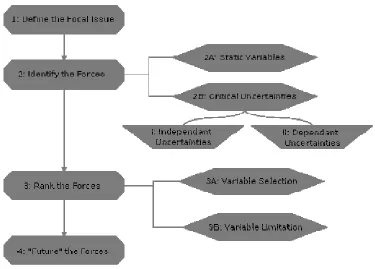
can be found in Table 3.1. A chart of the steps can be found in Figure 3.1.

Identifying the focal issue is the first step in typical scenario generation processes.

Once the focal issue has been defined, the next step is typically the identification and

classification of the variables related to that issue. First, the analyst must attempt to

identify the variables that have the highest level of impact on the focal issue. Next, those

(43)

ranked, the relationships between the variables are assessed and recorded. Finally, the

scenario generating or “futuring” technique is applied to the variables. Each of these steps

[image:43.612.86.498.178.581.2]

is discussed in more detail below.

Table 3.1: Works Consulted in Assembling the Scenario Method Overview

Authors Title Citation

Bartis, J. Long range energy R&D (42)

Boardman, A.,

Greenberg, H., Vining, A., and Weimar, D.

Cost-benefit analysis (43)

Eppen, G, Martin, R.’ and Schrage, L.

A scenario approach to capacity planning (44)

Fahey, L. Scenario learning (45)

Flower, J. Spinning the future (46)

Futures Group Scenarios (47)

Goodwin, P. and Wright, G.

Enhancing strategy evaluation in scenario planning

(48)

Kahn, H. On thermonuclear war (39)

Lempert, R., Groves, D., Popper, S.; and Bankes, S

A general analytic method for generating robust strategies and narrative scenarios

(49)

Lempert, R., Popper, S., and Bankes, S

Shaping the next 100 years (50)

Masch, V. Return to the “natural” process of decision-making leads to good strategies

(51)

Rausch, E Simulation and games in futuring and other uses

(52)

Schwartz, P. The art of the long view: Planning for the future in an uncertain world

(37)

Schwartz, P., Leyden, P., and Hyatt, J.

The long boom: A vision for the coming age of prosperity

(38)

Wack, P. Scenarios: Shooting the rapids (53)

(44)

[image:44.612.118.493.95.364.2]

Figure 3.1 Steps of the Generic Scenario Analysis Process

3.3.1 Defining the Focal Issue

The first step of the scenario analysis process is arriving at a clear definition of

the focal issue. The focal issue is defined as the central question that the analyst wants

answered. The focal issue does not necessarily have to be perfectly defined but should be

stated with sufficient clarity that the analyst can begin the process of narrowing down

appropriate variables. The formulation of the focal issue should be carried out with

respect to any limitations on the resources available to generating the scenarios, a concept

which will be discussed in further detail in later sections. For example, in the case of the

MUSES project (mentioned in Section 2.7), the focal issue was the question of what

types of impacts different greenhouse gas reduction policies would have on the

(45)

3.3.2 Identifying the Forces

The process of identifying the forces related to the focal issue can consist of a

variety of methods including: interviews, discussion groups, expert opinions and

traditional academic research. The initial goal of identifying the forces is to attempt to

gather as many potential variables as possible. The larger the initial pool of potential

variables is, the less likely it will be that later analyses will miss a critical relationship or

impact. Although the actual ranking of variables in terms of their impact on the modeling

system occurs in the next step; it is beneficial to gather information from experts in the

field and academic research as to which variables are most likely key to the focal issue.

Collecting the information along with the variables will save research time in later steps.

For example, variables for the MUSES project included material costs of vehicle

components, performance characteristics of engine types, criteria for consumer decision

making and recycling costs among many others. Several methods of variable collection

(46)

Table 3.2: Potential Variable Collection Methods

Common

Sense Decisions Policy Research Academic Testimony Expert Patterns Historical

Title

Qualita

tive

Qualita

tive

Blended Blended Quantita

tive

Type

Common Sense describes the

process of the individual

researcher looking at the

data and deciding whether it

will have a s

ignif

ican

t ef

fect.

Examining Policy Decisions

is the process by which the

analyst explores possible

governmental actions and

points of view on a topic Academic R

esearch cons

ists

of exploring journal articles

and books for the purpose of

discovering possible future

trends. fields. knowledgeable in their considered to be highly individuals who are thoughts and opinions of process of discovering the Expert Testimony is the variables. analyses performed on the is a series of regression method of ranking variables The Historical Patterns