Nuclear magnetic resonance microscopy

RIT Scholar Works

Theses

Thesis/Dissertation Collections

1999

Nuclear magnetic resonance microscopy

Stefanie VanGorden

Follow this and additional works at:

http://scholarworks.rit.edu/theses

This Thesis is brought to you for free and open access by the Thesis/Dissertation Collections at RIT Scholar Works. It has been accepted for inclusion in Theses by an authorized administrator of RIT Scholar Works. For more information, please contactritscholarworks@rit.edu.

Recommended Citation

SIMG-503

Senior Research

Nuclear Magnetic Resonance Microscopy

Final Report

Stefanie C. VanGorden

Center for Imaging Science

Rochester Institute of Technology

May 1999

Nuclear Magnetic Resonance Microscopy

Stefanie C. VanGorden

Table of Contents

Abstract

Copyright

Acknowledgement

Introduction

Background

Methods

Slice Thickness

In-plane Resolution

Bruker Equipment

Results and Discussion

Nylon Screw Phantom

Cone Phantom

Line/Glass Phantom

Organic Applications

Conclusions

References

List of Symbols

Appendix

Nuclear Magnetic Resonance Microscopy

Stefanie C. VanGorden

Abstract

Nuclear magnetic resonance (NMR) microscopy is magnetic resonance imaging (MRI) on a small scale. The purpose of this study was to develop an NMR microscope capable of producing tomographic images of 5 mm objects. The microscope was developed around an existing Bruker 300 MHz NMR spectrometer with a three orthogonal axis gradient coil set. Computer code for generating tomographic images was written and images were obtained of various standard test objects, referred to as phantoms. Phantoms were created to mathematically evaluate and document features such as in-plane resolution, and slice thickness. An in-plane resolution of 118 μm and a slice thickness of 0.8 mm were readily obtained on 5 mm diameter objects. Smaller values may be obtainable with signal averaging. Typical images are presented. The NMR microscope and software developed by this research is available in the RIT

Department of Chemistry for use by RIT faculty and students.

Copyright © 1999

Center for Imaging Science

Rochester Institute of Technology

Rochester, NY 14623-5604

This work is copyrighted and may not be reproduced in whole or part without permission of the Center for Imaging Science at the Rochester Institute of Technology.

This report is accepted in partial fulfillment of the requirements of the course SIMG-503 Senior Research.

Title: Nuclear Magnetic Resonance Microscopy Author: Stefanie C. VanGorden

Project Advisor: Joseph P. Hornak SIMG 503 Instructor: Joseph P. Hornak

Nuclear Magnetic Resonance Microscopy

Stefanie C. VanGorden

Acknowledgement

I thank Joseph Hornak for his support and input on this project.

Nuclear Magnetic Resonance Microscopy

Stefanie C. VanGorden

Introduction

Nuclear magnetic resonance (NMR) microscopy is magnetic resonance imaging (MRI) on a small scale (3). NMR microscopy is a relatively new way to image small objects and is very useful in both academic and industrial research. NMR microscopy is used by the food and agricultural industries as a tool for analyzing the amount and effect of water in their products. Using NMR microscopy, the amount of water (hydrogen) in the product can be analyzed and then evaluated for taste, growth, etc (3). This knowledge will allow researchers to vary production conditions and

hopefully yield a better product. The broad, long-term objective of this research is to develop NMR microscopy at the Rochester Institute of Technology (RIT) to a point where it is potentially useful to industry, especially analyzing food for water content.

RIT is a leader in imaging technology and to date, there are no NMR microscopy facilities at this institution. Currently, a Bruker 300 MHz NMR spectrometer is used to obtain spectra. Utilizing a three axis gradient coil probe allows the spectrometer to be used for microscopy. The main goal of this research is to document features such as slice thickness and in-plane resolution on the NMR microscope. This microscope will ideally be capable of producing a 1 mm thick, approximately 50 μm in-plane resolution tomographic image.

Background

Nuclear magnetic resonance imaging was developed in the early 1970's and was largely used for medical research on the human body (3). In 1986, MRI was done on a much smaller scale using NMR spectrometers essentially creating the field of NMR microscopy (3)(10)(13)(8)(12). NMR has widespread applications in gathering information about microscopic properties of biological tissues, pharmaceutical products, and agricultural products (9).

Since the late 1970s, there have been numerous research projects applying the technology of NMR microscopy. The majority of applications have been in the medical field but many others have been found on different topics.

Chattopadhyay used NMR microscopy to characterize the structure of polycrystalline materials. Others did research on time-independent point-spread functions and high-gradient NMR microscopy (12)(13). McFarland also did research on improving SNR and found spatial resolutions limits to be approximately 6 μm. T1 and T2 are parameters that are

varied to emphasize specific tissues over other ones. An article on multicellular tumors manipulated T1 and T2 and

documented an in-plane resolution of 14 μm (2). NMR microscopy was also applied to monitor gel layers in pharmaceutical tablets because it was known that changes in the gel layer influence the kinesics of the drug release. This research used an in-plane resolution of 70 μm and a slice thickness of 650 μm (1). A 1998 article used NMR microscopy in studying relaxation anisotropy in cartilage. A Bruker AMX 300 NMR spectrometer obtained a slice thickness of 1 mm and an in-plane resolution of 14 μm. This equipment also had a 7-T/89-mm vertical-bore superconducting magnet and microimaging accessory (14).

NMR microscopy utilizes a property found certain nuclei called spin. The governing equation for both MRI and NMR is

ν = γ B [1]

where B is the magnetic field strength, and γ

gyromagnetic ratio and also the strength of the magnetic field. Given a particular magnetic field strength (B), a particle having a net spin will absorb a photon of ν (8).

In NMR microscopy, a magnetic field is applied to a sample containing water (for example) and the property of spin causes protons (Hydrogen) in the water molecules to absorb a photon of frequency νa. With currently available NMR

magnets νa is in the range of 60 to 800 MHz (8). Absorption causes the proton to be excited to the next energy level

and all of the excited protons combined can be thought of as the net magnetization. The magnetic field is

conventionally placed in the z direction. At equilibrium, the net magnetization is zero Mo and when the system is not

at equilibrium the net magnetization is Mz. The equation governing the two relationships is

Mz = Mo ( 1-e-t/T1) [2]

where T1 is the spin-lattice relaxation time and represents the time needed to change Mz by a factor of e. T2 is the

spin-spin relaxation time and it is always less that T1. The equation governing T2 is

Mxy = Mxyoe-t/T2 [3]

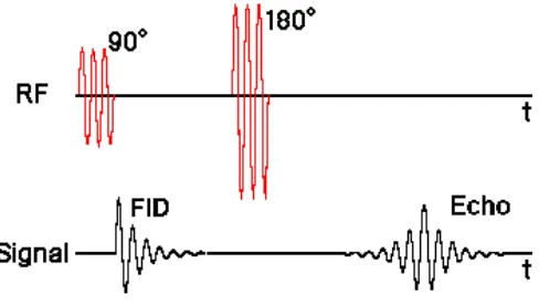
and this is the time needed to reduce the transverse magnetization by a factor of e. In order to determine the location of protons in the sample, pulsed magnetic fields of 90 degrees or 180 degrees are used. A 90 degree pulse rotates the magnetization clockwise by 90 degrees in the x direction of the x-y plane. A 180 degree pulse rotates the

magnetization by 180 degrees about the x axis. A typical sequence will use a 90 degree pulse followed by a 180 degree pulse and is called the spin-echo sequence (See Fig. 1).

Figure 1: Timing diagram for a spin-echo sequence (7).

Fig 1. is just a schematic diagram of a spin-echo sequence for spectroscopy. It is necessary to add two gradients to perform tomographic imaging. With the additions of three gradients, this sequence is what allows protons in a sample to be mapped to their x-y locations. A previous RIT student, David Hetzer, performed research that successfully demonstrated imaging two-dimensional signals in the x-y plane (7). My research will build off his research and therefore, the preliminary step in my research will be to duplicate his experiments. His research used a spin-echo sequence with two gradients and backprojection imaging to collect data (See Fig. Fig 2).

Figure 2: Example of backprojection imaging(8).

His research also documented that the relationship between frequency and position was a linear relationship

confirming that the gradient coils were working properly. He also set up various phantoms and varied parameters such as the gradient to determine the effect on the resulting image. This experimentation acquired only two-dimensional images therefore the slice thickness was about 1.5 cm. All of the information was averaged together in the z direction.

For tomographic imaging, the slice thickness (Thk) is specified and the signal is squished the width equal to Thk. Using the governing equation

ν=γ Βo, and substituting for Bo we yield

Δν=γ Thk Gi [4]

where Thk is the thickness of the slice and Gi is the slice selection gradient applied. By rearranging, we yield the

thickness as a function of the change in frequency (Δν) and inversely proportional to the slice selection gradient.

Thk = Δν/(γ Gi) [5]

Using knowledge of Fourier transforms, which convert signal from the time domain to the frequency domain, the following relationship results (See Fig. 5):

Δν = 2/ tw [6]

By further graphic interpretation, we can conclude that Δν = 2/tw and substituting this into Eq. 5 yields

Thk = 2/(γ Gi tw) [7]

which will allow us to calculate various parameters. We know that the gyromagnetic ratio is 42.58 Hz/T for hydrogen,

Gi is less than 50 x 10-4 T/cm, and tw is 10-6

seconds. Rearranging the equation and solving for the slice selection gradient yields Gi = 500 x 10-4 T/cm which

causes a problem because Gi

is greater than the maximum gradient of the system by a factor of ten. To compensate for this problem, we will have to utilize the equation

θ = 2π γ tw B1 [8]

where θ is equal to 90 degrees, tw is the amount of time the field is on, and B1 is specified in Figure 5 below. We will

make B1 larger which will make tw smaller and plugging into Eq. will yield a smaller Gi. This should yield a slice

Figure 3: (A) Shows the relationship the result of a Fourier Transform (B) Illustrates the relationship as a result of the FT.

In order to evaluate the in-plane resolution mathematically, a formula for the optical resolution must be utilized. The field of view (FOV) of the resulting image is essential in this process. The FOV is equal to the frequency of sampling fs, divided by the gyromagnetic ratio γ multiplied by the frequency encoding gradient Gf by definition.

FOV = fs / γ Gf [9]

Substituting into the above equation yields the optical resolution. The optical resolution (OR) is equal to the FOV

multiplied by the product of inverse of pi multiplied by the combined time constant T2* and the quantity divided by

the gyromagnetic ratio γ times the frequency gradient applied in the x direction Gνx.

OR = (FOV (πT2*)-1)/(γ Gνx) [10]

These variables are located in Fig. 4 for further clarification.

Figure 4: Illustration of the field of view and T2*.

The result of optical resolution calculated by Eq. 10 is the limit to how small the theoretical resolution will become. Substituting approximate values into the above equation yielded an optical resolution of roughly 20 μm.

Furthermore, the main goal of my research project is to produce one millimeter thick, 50 μm in-plane resolution Magnetic Resonance images using the Bruker 300 MHz DRX spectrometer. The in-plane resolution will approach 50 μm depending on the results acquired by phantoms and the limits placed by the spectrometer. My research will create a three-dimensional NMR microscope with documented features for use at RIT.

My experimentation has two major phases: documenting slice thickness of roughly 1 mm, and obtaining an in-plane resolution of approximately 50 μm. There are no human subjects required for these experiments. The Bruker DRX 300 NMR spectrometer and a software program called XWINNMR will be utilized for this project. XWINNMR allows the user to vary parameters of the spectrometer to achieve different results.

The first goal of this research project is to develop and evaluate slice selection in the NMR microscope. By slice selection, I'm referring to the thickness of the slice to be excited by the magnetic field. All other areas in the sample tube will remain unchanged. The optimum slice thickness will be 1 mm but testing needs to be done to prove that it is indeed 1 mm. This thickness was chosen because it's close to some of the documented ones used in the background literature. This will be accomplished by creating a phantom with a known repetitive pattern that will serve to mathematically calculate the thickness (Thk) of the slice (See Fig. 5).

Figure 5: Illustration of slice thickness.

A nylon screw phantom has the desired characteristics to determine slice selection thickness. The diameter of the nylon screw is less than 5mm and it has 32 threads per inch (TPI) which is about 1.2 threads per millimeter. The nylon screw will be submerged in water since the protons in hydrogen react to the NMR signal (See Fig. 6).

Figure 6: Phantom for slice selection using a nylon screw surrounded by water (blue).

The nylon screw phantom will be used to evaluate whether the theoretical calculations did yield a slice thickness of 1 mm. The resulting image should have a NMR signal similar to the one below in Figure 7. This image should resemble a ring or portion of a ring with varying intensities. Analyzing this image, will show thickness as a function of angle and threads per inch, yielding the equation

Thk = φ/360 * 1/TPI * 25.4 mm/In [11]

Figure 7: Resulting image of the slice selection phantom used to determine the thickness of the slice.

Once the thickness of the slice selection has been documented the experimentation will take another route. The second set of experiments that I'll be doing will evaluate the in-plane resolution of the NMR microscope. Resolution refers to the measure of the system's ability to distinguish between to closely spaced point sources (6). The fundamental limit to this system is that as size of the volume element gets smaller, its signal contribution is reduced and a reduction occurs in the signal-to-noise ratio (3). This phenomenon can be reduced using signal averaging. This will not be concentrated on in this experimentation though.

The theoretical resolution limit of this system is about 20 μms. To quantitatively test this limit, a specific phantom will be created. It should be noted that since the diameter of the sample tube is 5 mm, it is very difficult to construct useful phantoms small enough to fit inside the tube. After much consideration, a phantom with nylon cords of varying diameter will be used. The lower limit of cord diameter used will be approximately 45 μm or about the thickness of the diameter of glass rods. The upper limit will be approximately 139 μm for fishing line. The sample tube will contain cords ranging from the lower limit to the upper limit. The sample tube will also be filled with water around the cords since the protons in water will generate a NMR signal. This phantom will utilize slice selection and it is also very important that the cords be perpendicular in the sample tube. An illustration of the sample phantom is located in Figure 8 below.

Figure 8: Illustration of phantom to evaluate in-plane resolution.

Bruker Equipment:

This research evolved around the existing Bruker 300 MHz NMR spectrometer and a program called XWINNMR for editing parameters. A portion of the research time was spent learning how to operate the spectrometer, and use the software.

There are two probe heads on the spectrometer, one for taking spectra (qnp #7) and one for imaging (bbi #11). This spectrometer is normally used for taking spectra so the probe head was changed and replaced for each day of data collection.

Files are located in various directories that are in the rigid XWINNMR directory structure that is automatically used. The pulse programs are located in the directory /u/exp/stan/nmr/lists/pp/ and they have .ssse extensions. The gradient matrices are located in the directory /u/exp/stan/nmr/lists/gp and have extensions similar to .ssse.r. Images are located in /disk2/data/scv996/nmr/. The pulse programs and gradient matrices are located in the appendix.

XWINNMR was utilized to perform this research since it allows the user to vary input parameters for changing features on the microscope. The table below contains many of the commands that were used. Research was done in manual control mode that turns off the sweeping feature of the spectrometer.

Table 1: Common XWINNMR commands and their meanings.

XWINNMR Command _Description

rsh Read in shim file for a particular probe

wsh Write a shim file for a particular probe

edhead Change probe seen by the software

acq Shows the FID (Free induction decay) window

pulsdisp Allows the user to view a simulation or timing diagram

rga Receiver gain adjustment

wobb Allows user to tune the probe

halt Ends the wobb command

zg Runs the program specified in the eda display

eda and edp Used to change programs or length of pulses

xfb Performs the FT to turn resulting signal into an image for this research

NS Number of scans taken

DS Number of dummy scans

P1 Duration of the 90 degree pulse

P2 Duration of the 10 degree pulse

PL1 Amplitude of the above pulses

L1 Loop counter parameters (choose 4 and it'll perform 4*256 scans)

The time it takes for image collection varies. The user can specify the image size and the number of repetitions. Images collected were 256x256. It takes about 1.5 minutes to obtain an image. Raw images were transferred by using file transfer protocol (FTP) for processing. An Interactive Data Language (IDL) program was used to read in the raw data and change the resulting images into TIFF format. This IDL program is located in the appendix.

Results and Discussion

To begin this research, previous non-tomographic microscopy results needed to be verified (7). This research

essentially created a NMR microscope which would take the hydrogen signal from the entire sample tube range of 1.5 cm and average it to create an image. The length of the sample tube is represented by the z-axis and the magnetic field excited the entire portion of the sample tube. The resulting image has all the sample values in the z-direction averaged to yield one z value for each x-y location. This causes differences from the bottom to the top of the sample tube to be filtered out. The timing diagram for this pulse sequence is located in Figure 9. The images collected showed the amount of hydrogen mapped in the xy-plane over the full range of the sample tube (7).

Figure 9: Diagram illustrating the two-dimensional sequence.

Figure 10: Image with a horizontal artifact present.

Slice Thickness Documentation

Nylon Screw Phantom

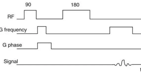
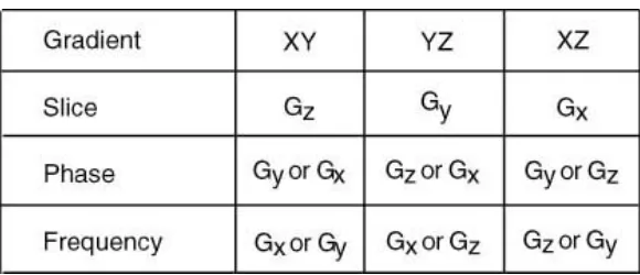
To create a tomographic NMR microscope, a slice selective gradient was applied in addition to the phase encoding gradient, and frequency encoding gradient (See Fig. 11). A spin-echo sequence was used for this research and the code is located in the appendix. This sequence, by manipulating the pulse width and the values for the slice selection gradient, caused a specific portion of the sample tube to be excited and created a tomographic NMR microscope. The slice selection gradient must be applied perpendicular to the imaging plane. The phase encoding and frequency encoding gradients need to be applied in the same plane as the slice but orthogonal to each other (See Fig. 12). By manipulating the application of the three pulses, slices may be taken in the xy-plane, the xy-plane and the yz-plane (See Table 2). Oblique imaging can also be implemented by applying combinations of the various gradients to yield the desired angles. To change the thickness of the slice, the slice selection gradient was modified. The thickness of the slice is found using the formula Thk = Δν/(γ

Gs) where the thickness is inversely proportional to the slice selection gradient. Gradient values implemented into the time sequence are percentages. The maximum gradient is 50 G/cm for this spectrometer and by using a slice selection gradient of 100%, the gradient applied will be 50 G/cm. Using a value of 10% would yield a gradient of 5 G/cm. Since thickness is inversely proportional to the slice selection gradient, implementing a value of 10% will yield a thicker slice than that of 100%.

Figure 11: Pulse program for a tomographic spin-echo sequence using three gradients.

Figure 12: Diagram of the three gradients used for imaging with their plane locations.

Table 2: Gradients for imaging in various Planes.

Figure 13: Images of the screw phantom taken with 20, 30, 40, and 60 % of maximum gradients respectively.

While trying to document the results from this phantom, it became apparent that if multiple turns were present in the image, there'd be no way to determine how many turns occurred. Also, the input for the 90 and 180 degree pulses is square. Therefore, the Fourier Transform of this input is a sinc function. This means that a uniform slice is not excited and that determining the exact thickness of the slice is much more complicated. Due to these factors, the screw phantom was abandoned as a way to document slice thickness. This phantom did serve to illustrate that by changing the z gradient, the signal-to-noise ratio varied from image to image as seen in Figure 13 above.

Cone Phantom

The difficulty documenting slice thickness due to the repeating threads on the screw phantom led to the

Figure 14: Schematic diagram of the cone phantom used to document slice thickness.

Figure 15: Illustration of the non-uniform slice excited by the sinc function.

Utilizing information about the sinc function (See Fig. 15), showed the relationship Δν=2/tw. By plugging it into Thk = Δν/(γ Gs), yielded Thk = (2/tw)/(γ

optimal goal, the above equation was rearranged to solve for the width of the pulse that would create a 1 mm slice. A gradient of 30 G/cm (gradient=60%) was used and the theoretical width of the pulse (tw) was calculated to be 157 μs. Therefore, by making the width of the 180 degree pulse 157 μs, the pulse sequence would theoretically yield a

thickness of 1 mm. The width of the 90 degree pulse is 7.5 μ s or half that of the 180 degree pulse. A gradient of 60% was used so that the thickness of the slice could increase or decrease without changing the width of the RF pulses. This result may be useful for more intricate studies but for this research, images were taken using a 180 degree pulse width of 160 μs and a 90 degree pulse width of 80 μs. The slice selective gradients varied the thickness from

approximately 0.01-0.59 mm. These pulse widths were used for all of the collected images and thicknesses seemed satisfactory to see changes in the images. For this piece of equipment, as mentioned previously, the maximum gradient is 50 G/cm but this number may not be exact although the theoretical calculations assume that it is. It should also be mentioned again that the pulses were square so a non-uniform thickness was excited in the sample causing the signal to be generated from an average of the thickness that followed a sinc pattern. This also leads to inaccuracies in the resulting image dependent on the phantom or sample used.

Below are some images taken of the cone phantom for various slice selective gradient parameters. Most of the

noticeable differences in the image result from the change in SNR for the different thicknesses. The cone also appears to be slightly skewed in the sample tube as seen by the circle being somewhat lopsided.

Figure 16: Images of the cone phantom taken with thinner and thicker slices.

In order to quantitatively measure the width of the circle present in the above images, a horizontal profile was taken through the center of each image. The horizontal profiles are located below in Figure 17. For these profiles, the x-axis represents the width of the image which is 256 pixels and the y-axis is the NMR signal created by hydrogen present in the water molecules of the excited slice. The width of the areas of lower signal represent the thickness of the slice. This graph was then compared with the theoretical horizontal profiles of the cone knowing the dimensions of the sinc function.

Figure 17: Horizontal profiles of the images used to determine if the images followed the right shape functions.

The top image in Figure 17 shows the horizontal profile for a thick slice and the lower image shows an image of thinner slice. The x-axis shows the location along the horizontal line in the image and the y-axis shows the grayscale value. The shape of these profiles matches the expected relationship. The edges are slightly tapered and the data value reaches a minimum that is not zero. Visible in the plots is the difference in the amount of signal-to-noise from varying the slice thickness. These slices vary from about 1 mm (Left) to a thin slice of ~0.3 mm (Right). These are theoretical values. Due to the small slice thickness relative to the geometry of the cone, there is not much difference in the width of the non-signal areas for the different thicknesses. These results make sense when conceptualizing the cone phantom. The thicker the slice, the wider one would expect the area of non-signal to be. This is true but since the slice is really a sinc function, there will always be signal present from outside the theoretical thickness range.

In-Plane Resolution Documentation

Figure 18: Skematic diagram illustrating fishing line phantom design.

Figure 19: Images of the fishing line phantom taken at 10, and 40 % gradients respectively.

Since this really was not a limiting resolution for the system, glass rods were stretched to diameters of ~50 μm and suspended in water. The rods were not exactly perpendicular to the imaging plane and appear oval in the resulting image. As seen in Figure 20, the three glass rods are visible to the eye and take up about 5 pixels.

Figure 20: Image of the glass rod phantom taken with 10 % gradient.

diameters small enough to be useful. Therefore, the smallest diameter object imaged was around 50 μm and the above images used for documenting slice thickness.

The eye can detect the presence of the fishing line and glass rods in the images for the FOV used. This however, doesn't give us an accurate portrayal of the relative size of these objects. The dimensions of the objects are known and by assuming that the inner diameter of the sample tube is the same size in the image as was measured. The inner diameter was measured as 4,250 μm and corresponds to approximately 179 pixels. Dividing these numbers yielded 23.7 μm/pixel which was used to calculate the size of the capillary tubes, fishing line, and glass rods. This formula is listed below in Eq. 12.

Image Size = (23.7 μm/pixel) * (Number of pixels in image) [12]

The calculated image size numbers should ideally match the measured dimensions of the objects and yield a slope of 1 for the graph. This was not the case. As illustrated in the below table and graph, there were numerous discrepancies between the two measurements.

Table 3: Calculated values for measured diameter [μ m] and image diameter [μ m].

Object Name

Object Size [μm] Image Size [μm]

Glass Rods 45 118

Small Line 87 248

Medium Line 126 379

Large Line 139 426

Inside dia. Cap. Tube 1000 900

Outside dia. Cap. Tube 1500 1398

Figure 21: Graphs of measured diameter [μ m] vs. calculated image diameter [μ m].

For the smaller objects, the image size is more than double that of the original size but for the larger measurements, the size in the image is smaller than the measured value. The glass rods measured 45 μm in diameter but are 118 μm in the resulting images. Therefore, the smallest in-plane resolution is 118 μm in the image and corresponds to

approximately 5 pixels. The cause of this discrepancy in size is unclear. It might be due to rods not being

perpendicular in the sample tube. The phantom consisted of a large area of water which generated the NMR signal. Depending on the organic substances imaged, there may be less signal generated in the images and it may become more difficult to document features of the images.

Errors were present in the images due to the fishing line or glass rods not being exactly perpendicular to the imaging plane. Also, this documentation used a fixed FOV which allowed the entire diameter of the sample tube to be present in the images. Modifying the FOV such that only one capillary tube is present in the image would likely increase the in-plane resolution. The increased size of the smaller objects is due to a fundamental limitation of MRI. This causes the objects to become smeared in the images and the exact reason is unknown. Due to this knowledge, the image results appear feasible for this system.

Organic Applications

Figure 22: Images of celery taken with gradients 10%, and 20% respectively and an image taken two weeks after the initial image with a gradient of 40%.

Conclusions

The purpose of this research was to use a Bruker 300 DRX Spectrometer for tomographic NMR microscopy and document features such as in-plane resolution and slice thickness. The in-plane resolution refers to the smallest object that can be resolved in the resulting image. Slice thickness for this research represents the amount of sample to get excited by the magnetic field documented in the z-direction. Ideal goals were a slice thickness of 1 mm and an in-plane resolution of 50 μm.

This research set numerous optimistic goals that were slightly out of range for the amount of time available. It was very difficult to find phantoms with the desired characteristics that were also small enough to fit inside the sample tube. It was also difficult to determine a slice thickness due to the pulse being shaped like a sinc in Fourier space and a non-uniform slice being excited from the phantom. Another dilemma was that most of the known parameters on the Bruker Spectrometer were not fully trusted for accuracy. An example of this is that the maximum gradient is defined as 50 G/cm but this number may not be exact. This value changes the theoretical calculations if inaccurate.

expected for the system given a non-uniform slice thickness. The horizontal plots of the images show both signal-to-noise changes between the images and also a relative shape that takes into account the slice thickness.

The next goal of this research was to document the in-plane resolution using a constant field of view. The major difficulties with this phantom were that it was difficult to find objects with the desired characteristics that were small enough to test the in-plane resolution limits. Initially, fishing line was imaged but the smallest diameter was 87 μm and the goal of the system was at least 50 μm. To test the limits further, glass rods were stretched and submerged in water since they were the smallest objects available for use with diameters of approximately 45 μm. Glass rods are visible in the resulting images. It was very difficult to keep the glass rods perpendicular in the sample tube and this is visible in the images by their oval shape. Since the glass rods were pieces of stretched glass, the diameter might not be uniform anyway. The calculated image size using the images shows that the in-plane resolution is 118 μm for a 45 μm object diameter. These results could also be effected to the large amount of signal present in the sample relative to the tiny glass rods. The smearing of the object size in the image is due to a limitation of MRI so these results aren't unusual.

Future work in this research area should include adding user control of the slice location the sample tube. Some ideas for this are in the following paragraphs.

Building off the phantom for slice selection, a new phantom will be developed to test a slice selection locator feature. Assuming that that the results from the first phantom adequately documented the thickness of the slice, this feature will allow the user to freely choose the particular location of the 1 mm slice. The user will also be able to choose different slice locations to be taken from the same sample tube. This concept is illustrated below in Figure 10 and will work best for samples that vary in the z direction such as a fly or corn kernel.

Figure 23:Fly with varying signal components in the z direction and illustration of the slice selection locator.

Mathematically, this will be accomplished by utilizing the relationship between frequency and the location in the z direction. The location in the z direction is equal to the change in frequency divided by the product of the

gyromagnetic ratio and the frequency gradient of the slice. Change in frequency will be equal to the frequency we apply minus a reference frequency at zero.

z = Δν/(γ Gslice) [13]

Δν = ν − νο [14]

Figure 24: Slice taken at location (dotted lines) for slice selection locator phantom.

Given that the thickness of the slice and the in-plane resolution are both accurately documented, the phantom

mentioned above should allow the specification to the location of the slice. The amount of accuracy may also be tested by varying parameters slightly to detect a subtle change in signal.

Nuclear Magnetic Resonance Microscopy

Stefanie C. VanGorden

References

1. Bowtell, R., et al. "NMR Microscopy of Hydrating Hydrophilic Matrix Pharmaceutical

Tablets." Magnetic Resonance Imaging. 12: 361-364 (1994).

2. Brandl, Matthias, et al. "Quantitative NMR Microscopy of Multicellular Tumor Spheroids

and Confrontation Cultures." Magnetic Resonance in Medicine. 34: 596-603 (1995).

3. Callaghan, Paul T. Principles of Nuclear Magnetic Resonance Microscopy . Oxford

University Press. NewYork: 1991.

4. Carter, Greggory A. and Douglas C. McCain. "Relationship of Leaf Spectral Ref lectance to

Chloroplast Water Content Determined Using NMR Microscopy." Remote Sensing

Environment. 46: 305-310 (1993).

5. Chattopadhyay, A.K., et al. "3-D NMR Microscopy Study of the Structural Characterization

of Polycrystalline Materials." Journal of Materials Science Letters. 13:

983-984 (1994).

6. Gaskill, Jack D. Linear Systems, Fourier Transforms, and Optics. John Wiley & Sons.

NewYork: 1978.

7. Hetzer, David. NMR Microscopy: Method Development for the Bruker 300MHz DRX

8. Hornak, J.P. The Basics of MRI, A Hypertext Book on MRI.

Http://www.cis.rit.edu/htbooks/mri/

9. Kuhn, Winfried. "NMR Microscopy- Theoretical Basis, 3D-Imaging and Applications."

Scanning. 13: 1-15 (1991).

10. Odoj, F., et al. "A Superconducting probehead applicable for Nuclear Magnetic Resonance

Microscopy at 7 T." Review of Scientific Instruments. 69: 2708-2712 (1998).

11. McFarland, E.W., and A. Mortara. "Three-Dimensional NMR Microscopy: Improving SNR

With Temperature and Microcoils." Magnetic Resonance Imaging, 10:

279-288 (1992).

12. McFarland, E.W. "Time-Independent Point-Spread Function for NMR Microscopy." Magnetic

Resonance Imaging. 10: 269-278 (1992).

13. Rofe, C.J., et al. "NMR Microscopy Using Large, Pulsed Magnetic-Field Gradients."

Journal of Magnetic Resonance, Series B. 108: 125-136 (1995).

14. Xia, Yang. "Relaxation Anisotropy in Cartilage by NMR Microscopy (

μ

MRI) at 14-

μ

m

Resolution." Magnetic Resonance in Medicine. 39: 941-949 (1998).

15. Zhou, Xiaohong, et al. "Three-Dimensional NMR Microscopy of Rat Spleen and Liver".

Magnetic Resonance in Medicine. 30: 92-97 (1993).

Nuclear Magnetic Resonance Microscopy

Stefanie C. VanGorden

List of Symbols

B = magnetic field strength

NMR = Nuclear Magnetic Resonance

MRI = Magnetic Resonance Imaging

γ

= gyromagnetic ratio

ν

= frequency

M

= net magnetization at equilibrium

M

= net magnetization not at equilibrium

M

=transverse magnetization

t = time

T

= spin-lattice relaxation time

T

= spin-spin relaxation time

Thk = slice thickness

G

= slice selection gradient

D

= change in frequency

t

= amount of time the magnetic field is on for

q = 90 degrees

p =3.14159...

pixel = picture element

FOV = Field Of View

OR = Optical Resolution

T

= the combined time constant

Nuclear Magnetic Resonance Microscopy

Stefanie C. VanGorden

Appendix

Slice Selective Pulse Program and Gradient Program for imaging in the xz-plane.

Slice Selective Pulse Program and Gradient Program for imaging in the xy-plane.

Slice Selective Pulse Program and Gradient Program with modified features for imaging in the xy-plane.

Program converting raw images to TIFF images

Original Slice Selective Pulse Program

Slice Selective Spin Echo Sequence

;jph.ssse ;grdprog: jph.ssse.r

;slice selective spin-echo sequence

;with Gz crusher pulses

1 ze

2 30m pl1:f1

3 d1

3u:ngrad ;slice selection on

p1 ph1 ;90 degree pulse

3u:ngrad ;phase and read on

d27 ;encoding time

3u:ngrad ;phase and read off

d2 ;recovery time

d10 ;delay to center echo (optional)

3u:ngrad ;Gz crusher on

d28 ;crusher time

3u:ngrad ;crusher off

p2 ph2 ;180 degree pulse

3u:ngrad ;Gz crusher on

d28 ;crusher time

3u:ngrad ;crusher off

d2

3u ph0

3u syrec

3u adc ph31

3u:ngrad ;read onxfb

aq ;aq=2*D27

d8

3u:ngrad ;read off

rcyc=2

100m wr #0 if #0 zd

lo to 3 times td1

30m rf #0

3m ip2 ;increment phase of 180 pulse by 90 degrees

3m ip31 ;increment phase of receiver by 180 degrees

3m ip31

lo to 2 times l1 ; loop for number of scans

exit

ph1=0

ph2=0

ph0=0

ph31=0

;use aqmod=qsim

;transform with: XFB and

; ssb1=ssb2=0 and wdw1=wdw2=SINE or QSIN

; si1=si2 (=td1)

; MC2=qf

; phmod(f1)=MC

; phmod(f2)=NO

Gradient Program for jph.ssse

jph.ssse.r

loop td1 <2D>

{

{(0) | (85) | (0)}

{(12) | (0)| (0), r2d(12) }

{(0) | (0) | (0)}

{(0) | (50) | (0)}

{(0) | (85) | (0)}

{(0) | (50) | (0)}

{(0) | (0) | (0)}

{(12) | (0) | (0)}

{(0) | (0) | (0)}

}

Slice Selective Pulse Program and Gradient Program

with Modified Features

;jph2.ssse ;grdprog: jph2.ssse.r

;slice selective spin-echo sequence

;with Gz crusher pulses

1 ze

2 30m pl1:f1

3 d1

3u:ngrad ;slice selection on

200u

p3:sp1 ph1 ;selective pulse

3u

3u:ngrad

d11

3u:ngrad ;phase and read on

d27 ;encoding time

3u:ngrad ;phase and read off

d2 ;recovery time

d10 ;delay to center echo (optional)

3u:ngrad ;Gz crusher on

d28 ;crusher time

3u:ngrad ;crusher off

p2 ph2 ;180 degree pulse

3u:ngrad ;Gz crusher on

d28 ;crusher time

3u:ngrad ;crusher off

d2

3u ph0

3u syrec

3u adc ph31

3u:ngrad ;read onxfb

aq ;aq=2*D27

d8

3u:ngrad ;read off

rcyc=2

100m wr #0 if #0 zd

lo to 3 times td1

30m rf #0

3m ip2 ;increment phase of 180 pulse by 90 degrees

3m ip31 ;increment phase of receiver by 180 degrees

3m ip31

lo to 2 times l1 ; loop for number of scans

exit

ph31=0

;td1 = td /2

;use aqmod=qsim

;transform with: XFB and

; ssb1=ssb2=0 and wdw1=wdw2=SINE or QSIN

; si1=si2 (=td1)

; MC2=qf

; phmod(f1)=MC

; phmod(f2)=NO

Gradient Program for jph2.ssse

jph2.ssse.r

loop td1 <2D>

{

{(0) | (0) | (40)}

{(0) | (0) | (-40)}

{(24) | (0), r2d(48) | (0)}

{(0) | (0) | (0)}

{(0) | (0) | (50)}

{(0) | (0) | (40)}

{(0) | (0) | (50)}

{(0) | (0) | (0)}

{(24) | (0) | (0)}

{(0) | (0) | (0)}

}

Slice Selective Pulse Program

;jph_xy.ssse ;grdprog: jph_xy.ssse.r

;slice selective spin-echo sequence

;with Gz crusher pulses

1 ze

2 30m pl1:f1

3 d1

3u:ngrad ;slice selection on

p1 ph1 ;90 degree pulse

3u:ngrad ;phase and read on

d27 ;encoding time

3u:ngrad ;phase and read off

d2 ;recovery time

d10 ;delay to center echo (optional)

3u:ngrad ;Gz crusher on

d28 ;crusher time

3u:ngrad ;crusher off

p2 ph2 ;180 degree pulse

3u:ngrad ;Gz crusher on

d28 ;crusher time

3u:ngrad ;crusher off

d2

3u ph0

3u syrec

3u adc ph31

3u:ngrad ;read onxfb

aq ;aq=2*D27

d8

3u:ngrad ;read off

rcyc=2

100m wr #0 if #0 zd

lo to 3 times td1

30m rf #0

3m ip2 ;increment phase of 180 pulse by 90 degrees

3m ip31 ;increment phase of receiver by 180 degrees

3m ip31

lo to 2 times l1 ; loop for number of scans

exit

ph1=0

ph2=0

ph0=0

ph31=0

;transform with: XFB and

; ssb1=ssb2=0 and wdw1=wdw2=SINE or QSIN

; si1=si2 (=td1)

; MC2=qf

; phmod(f1)=MC

; phmod(f2)=NO

Gradient Program for jph_xy.ssse

jph_xy.ssse.r

loop td1 <2D>

{

{(0) | (0) | (60)}

{(24) | (0), r2d(48) | (0)}

{(0) | (0) | (0)}

{(0) | (0) | (50)}

{(0) | (0) | (60)}

{(0) | (0) | (50)}

{(0) | (0) | (0)}

{(24) | (0) | (0)}

{(0) | (0) | (0)}

}

NMR Program to convert raw data to TIFF images

pro nmr_micro, input_filename, output_filename

;nmr_micro Reads nmr microscopy image in raw format and displays

;

; input: input_filename string variable with filename of raw

; data.

;

; output: result 65536 element long (4 bytes per pixel) array

; containing ASCII equivalent of the raw data.

;

; usage: nmr_micro, '2rr', 'screw_xz.tif'

;

;

c = intarr(256,256)

data = lonarr(65536)

;open and read raw data

openr, lun, input_filename, /GET_LUN ;, /XDR

print, 'reading file: '+input_filename

readu, lun, data

close, lun

free_lun, lun

;change byte ordering

byteorder, data

;print min and max values

themax=max(data)

themin=min(data)

print, 'max value= ',themax

print, 'min value= ',themin

; Display

k=0L

for i=0L, 254 do BEGIN

for j=0L,255 do BEGIN

k = k+1L

c(j,i) = data(k)

endfor

endfor

TVscl, c, 0, 0

; convert & write out

write_tiff,output_filename, bytscl(c)

;openw, lun, output_filename, /GET_LUN

; print, 'writing file: '+output_filename

;WRITEU, lun, c

;free_lun, lun

;print, 'finished writing file: '+output_filename

end