Shakedown solutions for pavements with materials following associated and non-associated plastic flow rules

This is a repository copy of Shakedown solutions for pavements with materials following

associated and non-associated plastic flow rules.

White Rose Research Online URL for this paper: http://eprints.whiterose.ac.uk/105961/

Version: Accepted Version

Article:

Liu, S, Wang, J, Yu, HS et al. (1 more author) (2016) Shakedown solutions for pavements with materials following associated and non-associated plastic flow rules. Computers and Geotechnics, 78. pp. 218-226. ISSN 0266-352X

https://doi.org/10.1016/j.compgeo.2016.05.005

© 2016. This manuscript version is made available under the CC-BY-NC-ND 4.0 license http://creativecommons.org/licenses/by-nc-nd/4.0/

eprints@whiterose.ac.uk https://eprints.whiterose.ac.uk/

Reuse

Unless indicated otherwise, fulltext items are protected by copyright with all rights reserved. The copyright exception in section 29 of the Copyright, Designs and Patents Act 1988 allows the making of a single copy solely for the purpose of non-commercial research or private study within the limits of fair dealing. The publisher or other rights-holder may allow further reproduction and re-use of this version - refer to the White Rose Research Online record for this item. Where records identify the publisher as the copyright holder, users can verify any specific terms of use on the publisher’s website.

Takedown

If you consider content in White Rose Research Online to be in breach of UK law, please notify us by

Shakedown solutions for pavements with materials following

associated and non-associated plastic flow rules

Shu Liu1,2, Juan Wang2,3Õ *,

, Hai-Sui Yu1, Dariusz Wanatowski1,3

1 _{The University of Nottingham, Nottingham, UK}

2 _{State Key Laboratory for GeoMechanics and Deep Underground Engineering, China University of Mining & Technology} 3 _{The University of Nottingham, Ningbo, China}

ABSTRACT: Existing lower-bound shakedown solutions for pavement problems are generally

obtained by assuming that materials obey associated flow rules, whereas plasticity of real

materials is more inclined to a non-associated flow. In this paper, a numerical step-by-step

approach is developed to estimate shakedown limits of pavements with Mohr-Coulomb materials.

In particular, influences of a non-associated flow rule on the shakedown limits are examined by

varying material dilation angle in the numerical calculations. It is found that the decrease of

dilation angle will lead to accelerated reduction of pavement shakedown limits, and the reduction

is most significant when the material friction angle is high. Furthermore, existing lower-bound

shakedown solutions for pavements are extended, in an approximate manner, to account for the

change of material dilation angle and the shakedown results obtained in this way agree well with

those obtained through the numerical step-by-step approach. An example of pavement designs

using shakedown theory is also presented.

Keywords: shakedown; pavements; non-associated flow rule; Mohr-Coulomb materials;

lower-bound

1 INTRODUCTION

Current mechanistic-empirical design methods for flexible pavements are usually conducted by

relating pavement life with elastic stress/strain at critical locations considering several principle

failure modes. However, one of the failure modes, excessive rutting, is mainly caused by an

accumulation of permanent deformation under repeated traffic loads. Therefore, a plastic design

2

distinguish the long-term elastic-plastic responses of a pavement to different levels of traffic

loads. If the load level is high, pavements may fail in a form of excessive rutting as a result of

accumulated permanent deformation. Alternatively, if the load level is low, the pavement may

deform plastically in the first number of load passes, then respond purely elastically to

subsequent traffic loads. The latter phenomenon is called ÔshakedownÕ, and the load below

which shakedown can occur is termed as Ôshakedown limitÕ. In the design of flexible pavements,

the shakedown limit can be calculated and checked against the design traffic loads to ensure very

small permanent deformations of pavements throughout their service lives.

The shakedown limit can be determined by either numerical elastic-plastic analysis (e.g. [3, 4])

or two fundamental shakedown theorems. MelanÕs static (lower-bound) shakedown theorem [5]

states that an elastic-perfectly plastic structure under cyclic or variable loads will shakedown if a

time-independent residual stress field exists such that its superposition with load-induced elastic

stress field does not exceed yield criterion anywhere in the structure. KoiterÕs kinematic

(upper-bound) shakedown theorem [6] states that shakedown cannot occur for an elastic-perfectly

plastic structure subjected to cyclic or variable loads if the rate of plastic dissipation power is

less than the work rate of external forces for any admissible plastic strain rate cycle. In the past

few decades, solutions for shakedown limits of pavements were developed mainly based on

these two fundamental shakedown theorems. Several different approaches based on MelanÕs

static shakedown theorem were developed for pavements subjected to two-dimensional (2D) and

three-dimensional (3D) moving surface loads [1, 3, 7-19]. Furthermore, kinematic shakedown

analyses were carried out by using KoiterÕs shakedown theorem for 2D and 3D pavement

[20-25]. It should be noted that the static and kinematic shakedown solutions provide lower and

upper bounds to the true shakedown limit of a pavement respectively. This is because the

lower-bound shakedown theorem satisfies internal equilibrium equations and stress lower-boundary

conditions, while the kinematic shakedown theorem satisfies compatibility condition for plastic

3

bound solutions have been obtained. For instance, when a 2D Mohr-Coulomb half-space is

subjected to a moving pressure, the lower-bound shakedown solutions (as obtained by Wang [3])

are identical to the upper-bound shakedown solutions (as obtained by Collins and Cliffe [21]).

Although some converged shakedown limits have been obtained by using the static and

kinematic shakedown theorems, they are calculated based on the assumption of an associated

flow rule (i.e. the plastic strain rate is normal to the yield surface). It is well known that granular

materials, such as soil and pavement materials, exhibit a non-associated plastic behaviour [26,

27]. Until now, very limited results have been reported on this topic. Boulbibane and Weichert

[28] proposed a theoretical framework for shakedown analysis of soils with a non-associated

plastic flow. It was reported by Nguyen [29] that this framework can be applied to shakedown

analysis of footing problems. With the use of linear matching method, Boulbibane and Ponter

were able to give 3D upper-bound shakedown solutions for Drucker-Prager materials with zero

dilation angle, but did not evaluate the influence of the change of dilation angle [22]. Numerical

studies of Li [25] extended the 2D upper-bound shakedown solutions of Li and Yu [24] to the

materials with non-associated plastic flow and suggested that the pavement upper-bound

shakedown limit is reduced due to the use of non-associated flow rule. For practical pavement

design, the influence of material plastic flow rule on lower-bound shakedown limits needs to be

assessed.

In this paper, first, shakedown limits for 2D pavement problems will be captured by using a

step-by-step numerical approach. Both associated and non-associated flow rules will be considered

for pavement materials. Then a direct method will be developed based on the previous work of

Yu and Wang [16] to estimate the lower-bound shakedown limits of pavements using a

4 2 PROBLEM DEFINITION

It is considered that a pavement is repeatedly subjected to a rolling long cylinder, as shown in

Figure 1. This can be simplified as an idealised plane strain pavement model with a moving

contact load P. The normal load distribution p (refer to Figure 2) can be assumed as:

), x' (

) / x' (

1 2

0 a a a

p

p= − − ≤ ≤ (1)

where a is half of contact length; p0 (= 2P/πa) is the maximum vertical stress located at xÕ = zÕ =

0. This load distribution is also known as 2D Hertz load distribution [1, 30].

3 NUMERICAL APPROACH

In this section, a numerical step-by-step approach for pavement shakedown problem is presented

and validated. Results including shakedown limits, residual stresses and plastic strains are

discussed in detail.

3.1 Method description

3.1.1 Numerical approach

Shakedown solutions based on the lower-bound (static) shakedown theorem were obtained by

assuming statically-admissible residual stress fields. It means the actual residual stress fields

developed in pavements were not considered. In the present study, finite element (FE)

elastic-plastic analyses are carried out to obtain the actual residual stresses developed in pavement

structures under repeated moving traffic loads. By using finite element software ABAQUS,

shakedown limits of pavements can be obtained through a step-by-step approach:

(1) As illustrated in Figure 2, for a given pavement structure, the load moves on the pavement

surface repeatedly from point B to point C. At the end of each load pass, the applied load is

removed thoroughly to investigate stresses remaining in the pavement (known as residual

5

(2) After a few numbers of load passes, a static load with the same magnitude of the moving

load is applied in the middle on the pavement surface. If no yielding point can be found in

the pavement (i.e. the total stress state of each point in the pavement does not violate the

yield criterion), a steady state (termed as Ôshakedown stateÕ) is achieved. In contrast, any

yielding point would indicate that the applied load is above the shakedown limit of the

pavement and the whole structure is in a non-shakedown state.

(3) Several numerical simulations with different load magnitudes are performed to determine the

shakedown limit of the pavement.

It should be noted this numerical approach requires great computation efforts in order to obtain

results with a reasonable accuracy. This problem has been solved to a great extent by using High

Performance Computing (HPC) facilities in the University of Nottingham, UK.

Figure 1 Idealised pavement model Figure 2 Model sketch and boundary conditions and

2D Hertz load distribution

3.1.2 Model description

A pavement model is established using ABAQUS. During every load pass, the load is gradually

applied at the start point, then translated in the horizontal direction at a constant speed, and

finally removed at the end point. The loading process is controlled by a user subroutine DLOAD.

The simulation is processed by means of Ôautomatic incrementation controlÕ with a given

maximum increment of 0.1. According to ABAQUS Analysis UserÕs Guide [32], the stiffness

matrix of the materials following associated plastic flow is automatically selected by the solver

(symmetric or unsymmetric), while for non-associated cases, it is set to be unsymmetric

z

x

xÕ zÕ oÕ p0

6

compulsively. Figure 2 shows a sketch of a two-layered pavement used in this study. A restraint

on horizontal movement is applied at two vertical boundaries, and a restraint on vertical

movements is applied on the bottom boundary. In order to minimise the influence of two

vertical boundaries on numerical results, no load is applied near the vertical boundaries.

Eight-noded, reduced-integrated, quadratic elements (CPE8R) are selected to avoid hour-glassing and

interlocking problems. Material properties of each layer are described by linear elastic

parameters (YoungÕs modulus E and PoissonÕs ratio ν) and Mohr-Coulomb criterion parameters

(cohesion c, friction angle ϕ and dilation angle ψ). The materials are assumed to be homogenous,

isotropic, and elastic-perfectly plastic with the associated plastic flow (i.e. ϕ = ψ) or a

non-associated plastic flow (i.e. 0 ≤ψ < ϕ). In this paper, subscript ÔnÕ of E, ν, c, ϕ and ψ represents

the nth layer. For single-layered pavement problems, identical materials are assigned to both

layers. In addition, tension is positive in the following results. It should be noted that the

Mohr-Coulomb model in ABAQUS uses a smooth plastic flow potential proposed by MenŽtrey and

Willam [31] which is very close to the classical Mohr-Coulomb model with faced flow potential,

especially when mean pressure is high [32].

The Drucker-Prager model with corresponding parameters transformed from Mohr-Coulomb

parameters was also used to investigate the influence of material plasticity model. Results

showed that these two models provide almost the same shakedown limits. For example, when ϕ

= ψ = 20¡, the shakedown limits are 7.5c in the case of Mohr-Coulomb materials and 7.4c in the

case of Drucker-Prager materials. Therefore, the Mohr-Coulomb model was selected in the

following study.

3.1.3 Validation

Table 1 shows different model dimensions used for sensitivity study and their corresponding

results. Model A was used by Wang and Yu [4] for homogenous half-space but required lots of

computation efforts. From Model B and Model C, it can be seen that some reductions in height

7

computation time. Therefore, model dimensions of 40a (length of loading area L) × 25a (depth H)

are selected. As mentioned before, the no-loading areas were applied near vertical boundaries.

Their influences were checked by Model D in which the moving load gradually entered through

the left boundary and finally exited through the right boundary, and Model E in which the length

of the no-loading area LÕ is increased from 3a to 10a. The results demonstrate the length of the

no-loading area barely affects shakedown limits. However, for some two-layered cases, it was

found that LÕ = 3a was not enough to prevent yielding near the vertical boundaries. Therefore,

Model E is finally chosen.

Sensitivity studies on mesh density were also carried out to ensure that mesh distribution can

obtain numerical results with a reasonable accuracy. High mesh density is applied in the first

layer and near the interface between two layers due to high stress and strain gradient. As shown

in Table 2 , the shakedown limit barely changes when the number of elements exceeds 16000 for

both single-layered and multi-layered model. Therefore, the mesh density in case 3 is selected. In

this case, elements are distributed uniformly along 10a≤ x ≤ 50a (the loading area) and small

elements (0.25a × 0.1a) are applied in the region near the surface (z ≤ 2a). The mesh is also fine

just beneath the interface, and it becomes coarser with increasing depth.

Table 1 Influence of model dimension (! = ψ = 20¼, ν = 0.3)

Model No. L H LÕ Theoretical

shakedown limit

Numerical shakedown limit

Average elapsed time per load pass (s)

A 78a 30a 3a

7.56c

7.5c 13854

B 40a 30a 3a 7.4c 3607

C 40a 25a 3a 7.4c 3576

D 40a 25a 0 7.5c 3480

E 40a 25a 10a 7.5c 3475

Table 2 Influence of mesh density

Case No. Number of Elements Theoretical shakedown limit Numerical shakedown limit

Average elapsed time per load pass (s)

Single-layered (! = ψ = 20¼, ν = 0.3)

1 1500

7.56c

7.2c 125

2 2500 7.2c 320

3 16000 7.5c 3475

4 18000 7.4c 3603

5 21600 7.4c 4714

Multi-layered

(E1/E2=0.5, ν 1=0.2, ν2 =0.49,

!1=ψ1=30¼,!!2=ψ2=0¼, c1/c2=1)

2 2500

8.48c2

8.5c2 344

3 16000 8.5c2 4279

6 20000 8.5c2 4561

Table 3 Comparison of numerical shakedown limits

8

distribution No. This study References (%)

1 Hertz \ 0 0 0.4 \ \ 4.0c 4.0c[1, 3, 7] ₀

2 Hertz \ 30 30 0.3 \ \ 10.6c 10.8c[1, 3, 13, 21] _1.8

3 Trapezoidal* \ 0 0 0.4 \ \ 3.7c 3.8c[15] 2.6

4 Trapezoidal* _{\ 15 15 0.3 \ \ 5.9c 6.2c}[15] _4.8

5 Trapezoidal* 1st 40 40 0.3 _{5 5 11.6c}

2 11.7c2[10] 0.8

2nd _{0 0 0.4}

6 Hertz 1

st

30 30 0.2 _{10 1 3.3c}

2 3.2c2[17] 3.0

2nd _{0 0 0.49}

*_{b/a=0.5 where a and b are the lengths of the lower and upper sides of trapezoid; Cases 1-4 are for single-layered pavements and cases 5-6 are for}

two-layered pavements

Shakedown limits obtained by the current approach are also compared with shakedown solutions

of other researchers. Those shakedown solutions were developed based on the classical

shakedown theorems and they all assumed that an associated plastic flow rule is applied to

pavement materials. Table 3 demonstrates that the differences between shakedown limits of the

current study and those in references are within 4.8%.

3.2 Single-layered pavements

Table 4 presents numerical results for single-layered pavements and compares them with the

shakedown limits of Wang [3]. If an associated flow rule (ϕ = ψ) is assumed, the shakedown

limits are only slightly lower than those in Wang [3] with a maximum difference of 2.0%.

However, if a non-associated flow rule (ψ <ϕ) is used in the numerical model, the difference can

be as high as 13.1%. Therefore, the effect of plastic flow rule cannot be neglected, especially

when the friction angle is high. Also, Table 4 exhibits that the dimensionless shakedown limit

(defined as the shakedown limit normalised by material cohesion ÔcÕ) accelerated reduces with

decreasing dilation angle, and the maximum reduction occurs when the dilation angle ψ drops

from 30¼ to 0¼ (friction angle ϕ remains 30¼).

Table 4 Material parameters and shakedown limits for single-layered pavements

Case No. ϕ (¡) ψ (¡) ν Theoretical shakedown limit Numerical Shakedown limit Difference (%)

1 30 30 0.3 10.82c 10.6c 2

2 30 20 0.3 10.4c 3.8

3 30 10 0.3 10.0c 7.6

4 30 0 0.3 9.4c 13.1

5 20 20 0.3 7.56c 7.5c 0.8

6 20 10 0.3 7.4c 2.1

7 20 0 0.3 7.2c 4.8

8 15 15 0.3 6.58c 6.1c 7.3

9 15 7.5 0.3 6.1c 7.3

9

According to the lower bound shakedown theorem, residual stress field σ_ijr _{(i and j denote x axis}

or z axis) plays an important role in helping structures reach the shakedown state. Ideally,

elements at the same depth should experience the same loading history; therefore the resulting

residual stress distribution should be independent of x axis [16]. Johnson [7] noted that σxzr and

σzzr should be zero for the 2D pavement problem due to the self-equilibrium condition. This was

verified by Wang [3] by numerical approach. Previous researches [3, 4, 34] demonstrated that

residual stresses in pavements under moving surface loads barely change after several load

passes, no matter the load applied is at or above the shakedown limit. It coincides with the test

report of Radovsky and Murashina [33] in which the measured residual stresses cease to increase

after 12 wheel passes. In consideration of the non-associated plastic flow, similar phenomenon is

also observed (Figure 3). Lower load level results in smaller amounts of residual stresses. When

the load magnitudes remain the same, the fully-developed residual stresses are also compared in

Figure 4(a) for the case of ϕ = 30¡ and p0 = 10.6c. Wang [3] also noted that the actual horizontal

residual stress field σxxr should lie between two critical residual stress fields (referred to as

Ôminimum larger root (MLR)Õ and Ômaximum smaller root (MSR)Õ) when the applied load is no

larger than the shakedown limit. Figure 4(b) further compare those residual stresses with MLR

and MSR when 0 ≤ z/a≤ 1. It is evident that the numerical residual stresses are completely

bracketed by MLR and MSR when the materials obeying the associated flow rule. It can also be

observed that the use of smaller dilation angle drifts some residual stresses further away from the

safe region bracketed by two curves. Therefore there are some critical depths below the

pavement surface representing locations for unlimited increasing plastic strains (Figures 5(a),

6(a)). If the load magnitude is higher than the shakedown limit, the structure will eventually fail

due to excessive cumulative permanent deformation. However, if the load magnitude is reduced

10

5(b), 6(b)). This is because smaller load magnitude will result in wider safe region between two

curves, so that the fully-developed horizontal residual stress field can be well contained.

Figure 3 Development of horizontal residual stress field

(a) (b)

Figure 4 Influence of dilation angle on horizontal residual stress field when φ! = 30¼, p0 = 10.6c

11

Figure 6 Development of plastic shear strains

3.3 Multi-layered pavements

A two-layered pavement structure with h1 = 2a, 1 = 30¡, ν1 = 0.2, 2 = ψ2 = 0¡, ν2 = 0.49 is

taken as an example for analyses. Results are obtained by using materials with either an

associated flow rule (ϕ1 = ψ1 = 30¼) or a non-associated flow rule (ϕ1 = 30¼ψ1 = 0¼). A direct

comparison between these two cases is made in Figure 7 for various stiffness ratios E1/E2.

Shakedown limits calculated through lower-bound approach of Wang and Yu [17] are also

presented in this figure as a dash line. In the present study, shakedown limit of any layer in a

multi-layered pavement is normalised by the cohesion of the second layer c2. It is noteworthy

that there exists an optimum stiffness ratio at around E1/E2 = 1.4 at which the shakedown limit is

maximised. The turning point also indicates the change of pavement failure mode from second

layer failure to first layer failure. As can be seen, numerical results for cases with associated flow

rule agree well with the lower-bound shakedown limits. However, when the non-associated flow

rule is applied, numerical results are lower than the lower-bound shakedown solutions when

E1/E2≥ 0.8. More results for multi-layered pavements with materials following associated flow

12

Figure 7 Comparison of numerical and theoretical shakedown limits for layered pavements when φ1 = 30¼, φ2 = 0¡,

c1/c2 = 1

Residual stresses also develop in multi-layered pavements. Taking a two-layered pavement as an

example, the fully-developed horizontal residual stress field exists not only in the first layer, but

also at the top of the second layer, as shown in Figure 8(a). This means that the top of the second

layer can also be critical. This agrees with the current pavement design approach (e.g. [35]) in

which the top of soil subgrade is considered as one of the critical locations. Again, with the use

of non-associated flow rule, some fully-developed residual stresses cannot reach the safe region

bracketed by MLR and MSR. Therefore, shakedown limits of the non-associated cases are

smaller than those using ϕ1 = ψ1. Further studies show that for the pavement with ϕ1 = 30¼ψ1 = 0¼,

if the load is decreased from 6.7c2 to 5.5c2, the numerical residual stresses can totally lie within

the safe region, as shown in Figure 8(b), and therefore the pavement will shake down to a steady

state.

In sum, the numerical approach is a valid way to obtain shakedown limits of pavements with the

assumptions of either an associated or a non-associated plastic flow rule. More numerical

solutions considering different load cases, strength ratios and layer configurations will be

13

Figure 8 Comparison between FE calculated residual stress field and critical residual stress fields when φ1= 30¼, φ2 = ψ2= 0¡, E1/E2 = 3

4 LOWER-BOUND SHAKEDOWN SOLUTIONS

The classical shakedown theorems follow the principle of maximum plastic work. Therefore,

shakedown solutions using classical shakedown theorems were based on the assumption of

associated flow rule. However, as explained in the previous section, ignorance of non-associated

plastic flow may overestimate the real shakedown limits of pavements thus lead to an unsafe

pavement design. The numerical approach developed in the previous section has been devoted to

overcome this issue. Despite much effort, very limited results have been reported in this aspect

due to computation cost. A direct method to address this issue would be more appealing for

practitioners. For this purpose, lower-bound shakedown solutions of Yu and Wang [16] will be

further developed in this section to obtain approximate shakedown limits for pavements

assuming non-associated plastic flow.

4.1 Shakedown analyses

Shakedown solutions of Yu and Wang [16] were developed based on MelanÕs lower-bound

shakedown theorem. Assuming Mohr-Coulomb materials following associated flow rule,

14 0, N M) (σr 2

xx + + ≤

=

f (2)

where _M λσ λσ _2tanφ(c λσe _tanφ)

zz e

zz e

xx − + −

= ; _{N 4(1 tan )[(} σ _{) (c} σe tan )2];

zz 2 e xz 2 φ

φ λ _{− −}λ

+ =

r xx

σ is self-equilibrated residual stress field; λ is a scale parameter; σe_ijis the elastic stress field

due to applied unit pressure p_0u; f is Mohr-Coulomb yield function. This problem then can be

solved by using a mathematical formulation developed in Yu and Wang [16].

In consideration of non-associated plastic flow, the dilation angle ψ(0 ≤ψ < φ) should be used.

Davis [36], Drescher and Detounay [37], Sloan [38] suggested the use of reduced strength (φ*

and c*) for the calculation of limit loads of structures in the case of materials obeying

non-associated flow rule. And it has been used for stability analysis of plane strain footing problem

(e.g. [37, 39-41]) in which:

, tan

tan

φ

η

φ

c,

c* =

η

. sin sin 1 cos cos φ ψ φ ψ η − = (5)

By replacing φ and c in Eq. (2) with φ* and c* and using a similar solution procedure in Yu and

Wang [16], shakedown limits of pavements λsdp0u with Mohr-Coulomb materials following

non-associated flow rule (defined by φ, ψ,c) can be found by searching through every point i at

each depth z = j in the half-space for the maximum value of λ in the following mathematical

formulation:

(

)

(

)

(

)

(

)

(

)

(

)

with _M σ σ _{2 tan (c} σe tan ),

zz 2 e zz e xx

* _{φ φ}

λ η

λ

λ − + −

= _{N 4(1 tan )[(} σ _{) (c} σe tan )2].

zz 2 2 e xz 2 2 * φ λ η λ φ

η − −

15

In the above formulation, max( M_i* N_i*) j

z= − − −

and min( M_i* N_i*)

j

z= − + −

are termed as Ômaximum

smaller root (MSR)Õ and Ôminimum larger root (MLR)Õ respectively. Any residual stress field

lying on or within the region bracketed by the MSR and MLR is a necessary condition for this

shakedown problem, because they are obtained by satisfying the equilibrium and boundary

conditions only. The actual residual stress field in a pavement should also be related with

material plastic deformation which is affected by loading history. It is also interesting to notice

that (e.g. Figure 4(b) and Figure 8), the actual residual stresses within the plastic region are very

close to the compressive (negative) MLR rather than MSR. This implies that the structure tends

to make a minimum plastic work (i.e. as small plastic deformation as possible) subject to a

certain level of load in order to achieve the shakedown state. Outside the plastic region, the

actual residual stresses are almost zero; whereas the MLR are positive. This is because the

assumption of yielding at all depths [16] yields some positive artificial residual stresses. In

reality, actual stress states at some depths will not touch the yield surface, reflected as zero

residual stresses.

4.2 Results and comparison

4.2.1 Single-layered pavements

A homogeneous half-space subjected to a moving 2D Hertz load is considered in this section and

the shakedown limit is usually denoted as a dimensionless parameter k = λsdp0u/c. Figure 9

compares dimensionless lower-bound shakedown limits with those obtained from numerical

approach and upper-bound solutions of Li [25] for various values of friction angle and dilation

angle. The results generally agree except the cases with high friction angle and low dilation

angle. This kind of discrepancy is also noted by other researchers (e.g. [38, 41]) when using the

16

0 5 10 15 20 25 30 35

0 2 4 6 8 10 12

Dilation angle ψ (¡)

D im en si o n le ss s h ak ed o w n l im it

Numerical results ( = 25¡) Theoretical results (φ = 20¡) Numerical results (φ = 20¡) Theoretical results (φ = 15¡) Numerical results (φ = 15¡) Upper bound (Li, 2010) Theoretical results (φ = 30¡)

Numerical results (φ = 30¡) Theoretical results (φ = 25¡) Numerical results (φ = 25¡) Theoretical results (φ = 20¡)

Figure 9 Comparison of theoretical and numerical shakedown limits for single layered pavements

Table 5 Dimensionless lower-bound shakedown limit parameters

φ ψ = 0¡ ψ = 5¡ ψ = 10¡ ψ = 15¡ ψ = 20¡ ψ = 25¡ ψ = 30¡ ψ = 35¡ ψ = 40¡ ψ = 45¡ 0¡ 4.00

5¡ 4.64 4.66

10¡ 5.34 5.42 5.45

15¡ 6.08 6.25 6.36 6.40

20¡ 6.84 7.14 7.36 7.51 7.56

25¡ 7.58 8.03 8.43 8.73 8.93 9.00

30¡ 8.25 8.90 9.50 10.02 10.44 10.72 10.82

35¡ 8.81 9.67 10.51 11.31 12.03 12.62 13.02 13.16

40¡ 9.21 10.28 11.39 12.51 13.60 14.60 15.44 16.02 16.24

45¡ 9.41 10.68 12.05 13.51 15.03 16.53 17.96 19.19 20.06 20.39

More dimensionless shakedown limit parameters are shown in Table 5 for the problem of

homogeneous Mohr-Coulomb half-space subjected to moving pressure. They can be expressed

as an analytical form:

. tan

σ σe_xz e_{zz φ}

η

η

k

+

= (7)

If this fictitious material (Eqs. (3)-(5)) is also applied to the upper bound shakedown solution of

Collin and Cliffe [21] where a tangential velocity jumpvcosφ is assumed, their solutions will

give the same shakedown limits.

4.2.2 Multi-layered pavements

Comparisons between lower-bound shakedown limits and numerical results for layered

pavements (with h1 = 2a) with various stiffness ratios also show good agreements in Figure 10.

Materials of the first layer have a friction angle = 30¡ and a dilation angle ψ = 30¡ or 0¡, while

17

the pavement structure is the minimum one among shakedown limits of all layers, and therefore

the turning point indicates the change of failure mode from one layer failure to another layer

failure; (2) The change of first layer dilation angle only changes static shakedown limits of the

first layer. When the first layer dilation angle is decreased from 30¡ to 0¡, lower-bound

shakedown limits of the first layer are well reduced. Since theoretical shakedown limits of the

second layer does not change, the turning points of non-associate cases are deviated from those

of associated cases. Therefore, the shakedown limits for non-associated cases are smaller than

those for associated cases when E1/E2 is relatively large (E1/E2≥ 0.8 in Figure 10), but remain

the same when E1/E2 is small enough or c1/c2 is large enough.

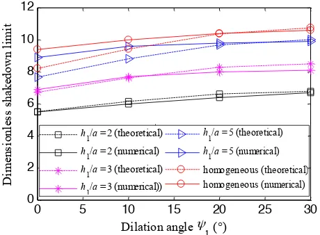
Two more models with h1 = 3a and 5a were established to evaluate the effect of layer

configuration on shakedown limits. As shown in Figure 11, the numerical shakedown limits

show good agreements with lower-bound shakedown limits when an associated plastic flow rule

is assumed. For non-associated cases, the numerical shakedown limits generally agree with the

lower-bound shakedown limits when h1/a = 2 and h1/a = 3. When the first layer is relatively

thick (i.e. h1/a = 5), the difference between theoretical and numerical solutions become obvious

with decreasing dilation angle. Indeed, the increase of the first layer thickness leads to even

more similar results to the homogeneous case.

In sum, when the dilation angle is at or above one third of the friction angle or the friction angle

is relatively low, the numerical and theoretical results generally agree well. Noticeable

discrepancy occurs when the friction angle is high while the dilation angle is very small in a

18 Theoretical results of 1st

layer (ψ1 = 30¡ )

Theoretical results of 2nd

layer

Numerical results (ψ₁ = 30¡) Numerical results (ψ

1 = 0¡) Theoretical results of 1st layer (ψ1 = 0¡ )

Figure 10 Comparison of theoretical and numerical shakedown limits with varying stiffness ratio when φ1 = 30¡, φ2

= ψ2 = 0¡, c1/c2 = 1

0 5 10 15 20 25 30

0 2 4 6 8 10 12

Dilation angle ψ₁ (¡)

D im en si o n le ss s h ak ed o w n l im it 1 h

1/a = 5 (theoretical)

h

1/a = 5 (numerical)

homogeneous (theoretical) homogeneous (numerical)

h

1/a = 2 (theoretical) h

1/a = 2 (numerical) h

1/a = 3 (theoretical) h

1/a = 3 (numerical))

Figure 11 Comparison of theoretical and numerical shakedown limits in two-layered pavements with varying first

layer thickness when φ1 = 30¡, φ2 = ψ2 = 0¡, E1/E2 = 3, c1/c2 = 1

4.2.3 Pavement design

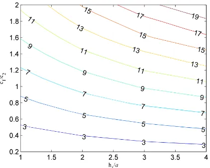
Design of layered pavements can be carried out through a thickness chart such as Figure 12.

Given elastic and plastic parameters of materials (En, νn, φn, ψn, cn), shakedown limits for

different first layer thicknesses can be determined from this chart and compared against the

design load. Finally, the thicknesses which can provide sufficient resistance to the maximum

design load (i.e. the shakedown limit is higher than the maximum design load) should be selected.

Compared with the results obtained using the assumption of φn = ψn, to sustain the same traffic

19

Figure 12 Contour of dimensionless shakedown limits as an example chart for the thickness design of a two-layered

pavement when φ1 = 44¡, ψ1 = 25¡, φ2 = ψ2 = 0¡, E1/E2 = 3

5 CONCLUDING REMARKS

In this paper, a numerical step-by-step approach and a lower-bound (static) shakedown approach

have been developed to obtain shakedown limits of single-layered and multi-layered pavements

assuming either an associated or a non-associated flow rule. Some important findings are

summarised as follows:

(1) The numerical approach presented in this paper is capable of obtaining shakedown limits of

single-layered or multi-layered pavements with either an associated or a non-associated flow rule.

(2) Compared with associated cases, the use of a non-associated flow rule obviously affects the

distribution of residual stress fields and therefore leads to a smaller shakedown limit. If the

friction angle is small or the difference between friction angle and dilation angle is small, the

variation of dilation angle will only slightly change the shakedown limit of the pavement.

Otherwise, the induced difference can be as high as 20.7%. Therefore, the influence of

non-associated plastic flow on the shakedown limit cannot be neglected, especially for materials with

zero dilation angles.

(3) The fully-developed residual stress field obtained from the numerical approach is bound by

two critical residual stress fields (i.e. MLR and MSR) when the pavement is in the shakedown

20

very close to MLR rather than MSR in the plastic region. This implies that a principle of

minimum plastic work may be applied when the structure tries to reach a shakedown state.

(4) Static shakedown solutions for pavements with materials obeying non-associated flow rule

have been developed by assuming fictitious materials with reduced strength. The results agree

with most shakedown limits obtained from the numerical approach and upper bound solutions of

Li [24]. When the dilation angle is much smaller than the friction angle (e.g. φ = 30¡ and ψ= 0¡),

the present shakedown solutions may underestimate shakedown limits of pavements.

Nevertheless, as a method to solve the pavement shakedown problem, the direct static

shakedown solutions can be very useful for conservative pavement design.

ACKNOWLEDGEMENTS

Financial supports from the National Natural Science Foundation of China (Grant Nos.

51408326 and 51308234), the State Key Laboratory for GeoMechanics and Deep Underground

Engineering, China University of Mining & Technology (Grant No. SKLGDUEK1411) and the

University of Nottingham are gratefully acknowledged. We are also grateful for access to the

University of Nottingham High Performance Computing Facility.

REFERENCES

1. Yu HS. Three-dimensional analytical solutions for shakedown of cohesive-frictional materials under moving surface loads. P Roy Soc A-Math Phy 2005; 461 (2059) : 1951-1964.

2. Brown SF, Yu HS, Juspi H, Wang J. Validation experiments for lower-bound shakedown theory applied to layered pavement systems.GŽotechnique 2012; 62 : 923-932.

3. Wang J. Shakedown analysis and design of flexible road pavements under moving surface loads. Ph.D. thesis, The University of Nottingham, UK, 2011.

4. Wang J, Yu HS. Residual stresses and shakedown in cohesive-frictional half-space under moving surface loads.Geomechanics and Geoengineering 2013a; 8 (1) : 1-14.

5. Melan E. Der spannungszustand eines hencky-misesÕschen kontinuums bei verŠnderlicher belastung.Sitzungberichte der Ak Wissenschaften Wien (Ser 2A) 1938; 147 (73).

6. Koiter WT. General theorems for elastic-plastic solids. In Progress in Solid Mechanics, Sneddon IN, Hill R, editors. North Holland : Amsterdam, 1960; 165Ð221.

7. Johnson KL. A shakedown limit in rolling contact. Proceedings of the Forth US National Congress of Applied Mechanics, 1962; 971-975.

21

9. Raad L, Weichert D, Najm W. Stability of multilayer systems under repeated loads. Trans Res B (NRC), TRB 1988; (1207): 181-6.

10. Yu HS, Hossain MZ. Lower bound shakedown analysis of layered pavements using discontinuous stress fields.Comput Method Apple M 1998; 167 (3Ð4) : 209-222.

11. Raad L, Weichert D, Haidar A. Analysis of full-depth asphalt concrete pavements using shakedown theory. Trans Res B (NRC), TRB 1989; (1227): 53-65.

12. Shiau S, Yu HS. Load and displacement prediction for shakedown analysis of layered pavements. Transp Res Record : J Trans Res B 2000; 1730 : 117-124.

13. Krabbenh¿ft K, Lyamin AV, Sloan SW. Shakedown of a cohesive-frictional half-space subjected to rolling and sliding contact. Int J Solids Struct 2007; 44 (11Ð12) : 3998-4008. 14. Nguyen AD, Hachemi A, Weichert D. Application of the interior-point method to

shakedown analysis of pavements. Int J Numer Anal Met 2008; 75 (4): 414-39. 15. Zhao J, Sloan SW, Lyamin AV, Krabbenh¿ft K. Bounds for shakedown of

cohesive-frictional materials under moving surface loads. Int J Solids Struct 2008; 45 (11Ð12) : 3290-3312.

16. Yu HS, Wang J. Three-dimensional shakedown solutions for cohesive-frictional materials under moving surface loads. Int J Solids Struct 2012; 49 (26) : 3797-3807.

17. Wang J, Yu HS. Shakedown analysis for design of flexible pavements under moving loads. Road Mater Pavement 2013b; 14 (3) : 703-722.

18. Wang J, Yu HS. Three-dimensional shakedown solutions for anisotropic cohesive-frictional materials under moving surface loads. Int J Numer Anal Met 2014; 38 (4) : 331-348.

19. Yu HS, Wang J, Liu S. Three-Dimensional Shakedown Solutions for Cross-Anisotropic Cohesive-Frictional Materials under Moving Loads. In Direct Methods for Limit and Shakedown Analysis of Structures 2015; p.299-313. Springer International Publishing. 20. Ponter ARS, Hearle AD, Johnson KL. Application of the kinematical shakedown theorem to

rolling and sliding point contacts. J Mech Phys Solids 1985; 33 (4) : 339-362.

21. Collins IF, Cliffe PF. Shakedown in frictional materials under moving surface loads. Int J Numer Anal Met 1987; 11 (4) : 409-420.

22. Boulbibane M, Collins IF, Ponter ARS, Weichert D. Shakedown of unbound pavements. Road Mater Pavement 2005; 6 (1) : 81-96.

23. Boulbibane M, Ponter ARS. Extension of the linear matching method to geotechnical problems.Comput Method Appl M 2005; 194 (45Ð47) : 4633-4650.

24. Li HX, Yu HS. A nonlinear programming approach to kinematic shakedown analysis of frictional materials. Int J Solids Struct 2006; 43 (21) : 6594-6614.

25. Li HX. Kinematic shakedown analysis under a general yield condition with non-associated plastic flow.Int J Mech Sci 2010; 52 (1) : 1-12.

26. Lade P, Nelson R, Ito Y. Nonassociated flow and stability of granular materials. J Eng Mech-ASCE 1987; 113 (9) : 1302-1318.

27. Lade P, Pradel D. Instability and plastic flow of soils. I : Experimental observations. J Eng Mech-ASCE 1990; 116 (11) : 2532-2550.

28. Boulbibane M, Weichert D. Application of shakedown theory to soils with non associated flow rules.Mech Res Commun 1997; 24 (5) : 513-519.

29. Nguyen AD. Lower-bound shakedown analysis of pavements by using the interior point method, Ph.D. thesis, RWTH Aachen Unviversity, Germany, 2007.

30. Johnson KL. Contact Mechanics. Cambridge University Press, 1985.

31. MenŽtrey P, and Willam, K. J. Triaxial failure criterion for concrete and its generalization. ACI Structure J 1995; 92 (3) : 311-318.

32. Abaqus 6.13 User's guide. SIMULIA. 2013.

33. Radovsky B, Murashina N. Shakedown of subgrade soil under repeated loading. Transp Res Record: J Trans Res B 1996; 1547 : 82-88.

22

35. Brown SF. Soil Mechanics in Pavement Engineering. GŽotechnique 1996; 42(3) : 383-426. 36. Davis EH. Theories of plasticity and the failure of soil masses. In Progress in Solid

Mechanics, Lee KI, editors. London: Butterworth, 1968; 341-380.

37. Drescher A, Detournay E. Limit load in translational failure mechanisms for associative and non-associative materials. GŽotechnique 1993; 43 (3) : 443-56.

38. Sloan S. Geotechnical stability analysis. GŽotechnique 2013; 63 (7) : 531-571.

39. Michalowski RL. An estimate of the influence of soil weight on bearing capacity using limit analysis. Soils Found 1997; 37 (4) : 57-64.

40. Silvestri V. A limit equilibrium solution for bearing capacity of strip foundations on sand. Can Geotech J 2003; 40 : 351-361.