Weak Interactions Based System
Partitioning Using Integer Linear
Programming
Romain Guicherd∗ Paul A. Trodden∗ Andrew R. Mills∗ Visakan Kadirkamanathan∗
∗Rolls-Royce University Technology Centre,
Department of Automatic Control & Systems Engineering, University of Sheffield, Mappin Street, Sheffield, S1 3JD, UK (e-mail:[email protected]; [email protected];
[email protected]; [email protected]).
Abstract:The partitioning of a system model will condition the structure of the controller as well as its design. In order to partition a system model, one has to know what states and inputs to group together to define subsystem models. For a given partitioning, the total magnitude of the interactions between subsystem models is evaluated. Therefore, the partitioning problem seeking for weak interactions can be posed as a minimization problem. Initially, the problem is formulated as a non-linear integer minimization that is then relaxed into a linear integer programming problem. It is shown within this paper that cuts can be applied to the initial search space in order to find the least interacting partitioning; only composed of controllable subsystems. Two examples are given to demonstrate the methodology.
Keywords:Decoupling problems, linear multivariable systems, decentralized control, integer programming.
1. INTRODUCTION
Systems models are widely used in control design espe-cially with the development of techniques such as model predictive control (Rawlings and Mayne (2009)) (Ma-ciejowski (2002)). Systems are growing in size and com-plexity and they are in most cases composed of interact-ing subsystems (Scattolini (2009)). For these large scale systems, the design of a centralized controller can be pro-hibitive due to the heavy computational resources required (Mayne (2014)). Also, if the system is geographically spread out, communication delays between the centralized controller and the actuators and sensors arise. One way to solve this problem is to see the system as a concatenation of subsystems and to design local controllers for each subsystem. In a top-down approach the full model of the multivariable system is partitioned into subsystem models so that the decentralized controller can be designed. De-centralized control has been studied for decades and design procedures have been established (ˇSiljak (1991)) (Bakule (2008)). However, the system model partitioning problem has been overlooked, often because the system is already composed of physical subsystems. Every subsystem model is defined by a set of states and inputs. The weak in-teraction partitioning problem consist of defining these sets in order to minimize the coupling between subsystem models. For instance, strongly coupled subsystem models can emerge from the main system model, particularly within chemical plants (Stewart et al. (2010)) or heating systems (Moro¸san et al. (2010)). The ideal partitioning of a
system model would yield completely decoupled subsystem models.
parts of the system. The attribution of weights within the interaction matrix is used in order to perform clustering and achieve system decomposition. Other work on decen-tralized control combined the controller design along with the controller topology, these two aspects are combined in the optimization function yielding a trade-off between the need for feedback links and the loss of performance com-pared to the centralized controller (Schuler et al. (2014)). Finally, other works have studied the actuator partition-ing problem (Jamoom et al. (1998)) (Motee and Sayyar-Rodsari (2003)). To the best of the authors’ knowledge the problem addressing state space model partitioning has not been studied. Therefore this partitioning approach is a standalone work, making any comparison difficult.
In this paper, we propose an integer programming based approached to the problem of partitioning a system model into a set of non-overlapping but coupled subsystem mod-els. The objective is to reduce the magnitude of the inter-actions between the subsystem models. Finally, cuts are added to rule out non-controllable partitionings in order for the algorithm to yield only controllable subsystem models.
The paper is organised as follows. Section 2 states the problem and section 3 introduces the required notations. Section 4 demonstrates how the problem can be relaxed into a linear integer programming problem. In section 5 the controllability cut principle is presented allowing to obtain controllable subsystems, section 6 explains the linear partitioning algorithm. In order to illustrate the algorithm section 7 includes some examples, finally section 8 concludes the paper.
Notation: For (a, b)∈ N2 such that a < b, the set Ja;bK defines the set containing the integers fromatobincluded. The operator|.|is used to denote the magnitude of a com-plex number when applied to a comcom-plex number. When applied to a matrix the magnitude operator is applied to all the matrix elements then summed. The operator k.k2
defines the Euclidean norm for complexes, vectors and ma-trices. For a setN, the notationN∗definesN/{0}. The su-perscript|represents the transpose of a vector or matrix.
A matrix B ∈ Rn×m will be noted (bij)(i,j)∈J1;nK×J1;mK and (Bkl)(k,l)∈J1;NK×J1;MK, respectively for the element and block notations, withN row blocks andM column blocks. For all n ∈ N∗ and A ∈ Rn×n, trace(A) denotes the sum of all the diagonal elements of A. For all (n, m) ∈
(N∗)2 andA ∈
Rn×m, rank(A) denotes the dimension of the vector space spanned by the columns of A. For any (i, j, k) ∈ (N∗)3 and (A, B) ∈
Ri×j×Ri×k the notation [A|B] defines the matrix obtained by concatenatingAand B horizontally. For any couple of integers (i, j)∈N2,δ
ij
denotes the Kronecker delta function.
2. PROBLEM STATEMENT
Given a linear time invariant controllable state space model defined by
˙
x=Ax+Bu (1)
where the matrix A is the state matrix and the matrix B is the input matrix respectively with the appropriate
sizes for N states andM inputs, therefore,x ∈ RN and u ∈ RM. Partitioning the system model (1) consists of decomposing the inputs as well as the states into groups representing subsystems. For a given number of partitions P ∈J2; min(N, M)Kand for any subsystemp∈J1;PKthe modelpcan be expressed as follows
˙
xp=Appxp+Bppup+ P X
j=1
j6=p
Apjxj+Bpjuj (2)
with for allp∈J1;PK,xp∈RNp andu
p∈RMp such that
P X
p=1
Np=N (3a)
P X
p=1
Mp=M (3b)
The weak interaction partitioning problem consists of minimizing the magnitude of the right-hand side sum in (2) for the subsystems while keeping each of them controllable. A non-overlapping condition for the states and the inputs is imposed by (3). The next section presents the decision variables, the constraints as well as the interaction metric necessary to formulate the weak interactions optimization problem.
3. WEAK INTERACTIONS PROBLEM FORMULATION
3.1 Decision variables
A decision variable is associated to the couples formed by a grouppand a stateias well as a grouppand an inputk. All the decision variables are binary variables. They are organised in two grouping matrices, the state grouping matrix α ∈ J0; 1KP×N and the input grouping matrix
β ∈ J0; 1K
P×M. Therefore, the rows of αand β represent
theP groups and the columns respectively represent the N states and theM inputs. For example withP = 3 and N = 5 a non-overlapping state grouping matrix could be
α=
0 0 0 1 0 1 1 1 0 0 0 0 0 0 1
!
3.2 Partitioning constraints
The formulation of constraints on the decision variables is necessary in order for the algorithm to return a solution complying with the rules defining non-overlapping subsys-tem models.
1. Each state group contains at least a state, hence, no state group can be empty and the partitioning has the correct number of state groups
∀p∈J1;PK,
N X
i=1
αpi ≥1 (4a)
2. Each input group contains at least an input, hence, no input group can be empty and the partitioning has the correct number of input groups
∀p∈J1;PK,
M X
i=1
βpi≥1 (4b)
3. A state can be in only one state group, therefore, the multiple use of a state is prevented and the non-overlapping requirement is respected
∀i∈J1;NK,
P X
p=1
αpi≤1 (4c)
4. An input can be in only one input group, therefore, the multiple use of an input is prevented and the non-overlapping requirement is respected
∀i∈J1;MK,
P X
p=1
βpi≤1 (4d)
5. Each state must belong to a state group, conse-quently, no state is left out of the optimization prob-lem
∀i∈J1;NK,
P X
p=1
αpi≥1 (4e)
6. Each input must belong to a input group, conse-quently, no input is left out of the optimization prob-lem
∀i∈J1;MK,
P X
p=1
βpi≥1 (4f)
The constraints are expressed for the two grouping matri-ces, however only three different sets of constraints concern each type of grouping matrix. Becauseαandβ are arrays of binary variables a natural implicit constraint linksN, M andP.
1< P ≤min(N, M) (5)
Subsystem interactions can come from the state matrices or the input matrices, the next subsection presents how these interactions can be formulated firstly using the block matrix form and secondly using the state space model elements.
3.3 Objective: minimizing subsystem interactions
The first part of the interactions comes from the state matrices. The subsystem model (2) presents the couplings
with the other subsystems in the form of a sum, this sum can be split into the state interactions and the input interactions. For a given number of partitions P ∈
J2; min(N, M)Kand for any subsystemp∈J1;PKthe state interactions can be expressed by
Jpstate=
P X
j=1
j6=p
|Apj| (6)
The expression written in block matrix form can also be represented using the state matrix elements as well as the state grouping matrix elements as follows
Jpstate=
N X
i=1
N X
j=1
αpi|aij|(1−αpj) (7)
The elements from the state grouping matrix are used here as boolean tests to take into account only the interactions acting on the subsystempand coming from the other sub-system states. A similar reasoning is applied to quantify the interactions coming from the input matrices
Jpinput=
P X
j=1
j6=p
|Bpj| (8)
In a similar fashion, (8) can also be represented using the input matrix elements as well as the elements of the state grouping matrix combined with the elements of the input grouping matrix, such that
Jpinput =
N X
i=1
M X
k=1
αpi|bik|(1−βpk) (9)
Likewise, the elements from the state grouping matrix combined with the elements of the input grouping matrix are used as boolean tests to take into account only the interactions acting on the subsystem pand coming from the other subsystem inputs. After having defined the two types of interactions, the full interaction metric can be calculated. Consequently, the last step is to pose the weak interactions optimization problem like it is presented within the next subsection.
3.4 Weak interactions optimization problem
The overall formulation of the weak interactions optimiza-tion problem is obtained by summing the interacoptimiza-tions com-ing from the states and the inputs over theP subsystems
Jinteraction=
P X
p=1
Jpstate+Jpinput (10)
min
α,β P X
p=1
N X
i=1
αpi hXN
j=1
|aij|(1−αpj)
+
M X
k=1
|bik|(1−βpk) i
s. t. (4)
(11)
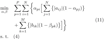
As it was demonstrated previously within this section the partitioning problem can be expressed as an integer opti-mization problem. However the cost function representing the interaction metric is non-linear, therefore the problem can be intractable. As it is presented within the next section a linear relaxation of the optimization problem (11) is made possible throughout the use of auxiliary variables.
4. LINEAR RELAXATION OF THE WEAK INTERACTIONS PROBLEM
The weak interactions optimization problem formulated previously (11) can be turned into a linear optimization problem, this is made possible due to the introduction of auxiliary variables. Replacing a product of binary variables by an auxiliary variable is a well known technique that requires the use of new linear constraints (Williams (2013)) (Bemporad and Morari (1999)) (Cavalier et al. (1990)). Two auxiliary binary variables are created along with their linear constraints.γis the binary variable used to take into account the interactions coming from the state matrix. As it is presented in Table I and in (12), γ is linked to α throughout four constraints. Indeed, four inequalities are necessary because of the four possible outcomes for the binary productαpi(1−αpj) in (11).
[image:4.595.79.292.72.153.2]From top to bottom within Table I, the four different cases are, first when no states belong to the group p then no interaction has to be accounted for. If the state i is not in the group p but the state j is, then no interaction is accounted for as this will be taken into account in the symmetrical case. If the stateibelongs to the grouppand the statej does not then an interaction is accounted for. The last case possible is when the two statesiandj both belong to the groupp, in this last scenario no interaction subsists as they are both in the same group.
Table 1. Auxiliary variableγ
Primary Auxiliary
αpi αpj αpi(1−αpj) γpij
0 0 0 0
0 1 0 0
1 0 1 1
1 1 0 0
The linear constraints for the auxiliary variableγ are the following
∀(p;i;j)∈J1;PK×J1;NK×J1;NK,
γpij ≤αpi+αpj (12a)
γpij≤1 +αpi−αpj (12b)
γpij ≥αpi−αpj (12c)
γpij≤2−αpi−αpj (12d)
In a similar way, δ is the auxiliary binary variable tak-ing into account the interactions comtak-ing form the input matrix. This time the constraints are formed using α as well as β because the input interactions are also state dependant. The same reasoning applies to formulate the four inequalities arising from the binary product αpi(1−
βpk) in (11).
Table 2. Auxiliary variableδ
Primary Auxiliary
αpi βpk αpi(1−βpk) δpik
0 0 0 0
0 1 0 0
1 0 1 1
1 1 0 0
The four linear constraints associated toδare represented in (13).
∀(p;i;k)∈J1;PK×J1;NK×J1;MK,
δpik≤αpi+βpk (13a)
δpik≤1 +αpi−βpk (13b)
δpik≥αpi−βpk (13c)
δpik≤2−αpi−βpk (13d)
Both auxiliary variables have three indexes and can be represented by cubic arrays of binary variables, their respective sizes are P ×N ×N for the state auxiliary variableγ andP×N×M for the input auxiliary variable δ. In addition to the constraints presented in (12) and (13), both auxiliary variables have to be composed only of binary variables.
The optimization problem presented in (11) is reformu-lated into the linear integer optimization problem pre-sented in (14), obtained by replacing the binary products by the auxiliary variables along with their constraints.
min
α,β P X
p=1
N X
i=1
N
X
j=1
γpij|aij| + M X
k=1
δpik|bik|
s. t. (4),(12),(13)
(14)
As it was presented within this section, the use of two auxiliary variables enables the linearisation of the opti-mization problem. The miniopti-mization problem presented in (14) because of the use of primary and auxiliary binary variables allows to trade non-linearities for an increase in variable size. Nonetheless the complexity of the optimiza-tion problem can be reduced by exploiting the structure of the plant model and by creating only the auxiliary variables where the state space model elements are not equal to zero. For instance, ifaij = 0 there is no need to
create (γpij)p∈J1;PK, similarly if bik= 0 with (δpik)p∈J1;PK. The next section presents the notion of controllability cuts reducing the search space in order to obtain only controllable subsystems.
5. CONTROLLABILITY CUT
[image:4.595.319.554.505.553.2]unfortunately no information is given concerning their controllability. The state space model of any subsystemp, represented without the couplings coming from the other subsystems can be rewritten from (2) as follows
∀p∈J1;PK,x˙p=Appxp+Bppup (15)
The controllability of any given subsystem modelpyielded by the optimization problem can be checked by verifying that the controllability matrixCp defined in (16) has full
row rank.
∀p∈J1;PK, Cp= [Bpp|AppBpp|. . .|ANppp−1Bpp] (16)
Therefore, at the end of the optimization process, a con-trollability test is performed for each subsystem model, testing that the set of equalities given in (17) holds.
∀p∈J1;PK, rank(Cp) =Np (17)
As one can see the controllability matrices Cp as well
as the integers Np representing the number of states in
subsystem p are results of the optimization and are not known a priori. Therefore implementing constraints within the linear integer optimization problem in order to restrain the solutions to the set of controllable subsystems is a tremendously difficult task. However, applying controlla-bility cuts to the search space recursively and a posteriori is possible.
Every time a non-controllable partitioning is achieved new linear constraints are added to the existing ones in order to reduce the search space by cutting the non-controllable partitionings out with an affine hyperplane. The principle of cutting solutions out of the search space is similar to the Gomory cuts (Gomory (1958)) where cuts are used to discard solutions that are not integer. Controllability cuts are applied from the root node and are valid for the entire search tree, hence cuts lifting methods are not necessary in this case (Balas et al. (1996)).
Grouping matrices can be seen as a concatenation of basis vectors, such that
α= [ei1|ei2|. . .|eik|. . .|eiN]ik∈J1;PK (18a) β = [ei1|ei2|. . .|eik|. . .|eiM]ik∈J1;PK (18b) with (eik)ik∈J1;PK the canonical orthonormal basis of R
P.
Subsequently the square of their 2-norm is equal to respec-tivelyN andM as it is calculated in (19) (20).
kαk22=trace(α|α) =
N X
k=1
e|i
k.eik=
N X
k=1
δikik=N (19)
kβk2
2=trace(β|β) =
M X
k=1
e|i
k.eik=
M X
k=1
δikik =M (20)
The set of non-overlapping grouping matrices of size P×
N and respecting the constraints (4a) (4c) (4e) will be referred to as GP N with GP N ⊂ J0; 1K
P×N. For a given
non-controllable optimal partitioning denoted byαnc∗and
βnc∗, and for any couple of non-overlapping grouping matricesαandβ, the inequalities (21) and (22) hold.
∀(αnc∗, α)∈G2P N,
trace(αnc∗|α) =
N X
k=1
e|i
knc∗.eik =
N X
k=1
δiknc∗ik≤N (21)
∀(βnc∗, β)∈G2
P M,
trace(βnc∗|β) =
M X
k=1
e|i
knc∗
.eik=
M X
k=1
δi
knc∗ik ≤M (22)
In addition, the upper bound is only reached in (21) when α=αnc∗ and in (22) whenβ =βnc∗. Consequently there exists a natural way of constructing affine cutting hyper-planes (23) when a non-controllable optimal partitioning (αnc∗, βnc∗) is obtained.
∀(α, β)∈GP N×GP M,(α, β)6= (αnc ∗
, βnc∗)
⇔trace(αnc∗|α) +trace(βnc∗|β)≤N+M −1 (23a)
⇔
P X
p=1
N
X
i=1
αncpi∗αpi + M X
k=1
βpknc∗βpk
≤N+M−1 (23b)
Every time a non-controllable partitioning is obtained a controllability cut (23) is added to the linear constraints before the optimization is computed again. Therefore, the previous non-controllable optimal partitioning can no longer be reached as it is now excluded from the search space. However because the groups are not ordered the same result can be achieved again simply by swapping the rows ofαandβ, leading to another representation of the same partitioning. Indeed, without any order constraints on the groups, P! identical representations of a single partitioning are possible.
6. PARTITIONING ALGORITHM
The algorithm implemented to perform the system parti-tioning takes the main state space model as well as the group numberP as inputs. It returns the state and input grouping matricesαandβonce one of the least interacting controllable partitioning is reached. The algorithm can be described by steps as it is computed. The first step is to build the linear constraints that will be used for the primary and auxiliary variables. Then the optimization is performed yielding the subsystem models as well as their controllability matrices. The last step of the algorithm is to add the appropriate set of controllability cuts if the optimal partitioning presents at least one uncontrollable subsystem as well as to go back to the previous step. Otherwise, the algorithm returns the least interacting con-trollable partitioning as a final result if the optimal parti-tioning obtained has all its subsystem models controllable.
The weak interaction partitioning problem is a 0-1 integer linear programming problem. The partitioning algorithm is presented below in algorithm 1.
Algorithm 1Partitioning algorithm Input :A, B, P
Output:α, β
while ∃p∈J1;PK, rank(Cp)6=Np do
if ∃(αnc∗, βnc∗)then
Add controllability cuts (23)
Run the optimization problem (14) subject to (23) Extract the subsystem state space models and compute:∀p∈J1;PK, Cp
else
Run the optimization problem (14)
Extract the subsystem state space models and compute:∀p∈J1;PK, Cp
end end
On the very first loop iteration, no solution exists, there-fore, the optimization is performed and the first grouping matrices are obtained. The next step is to check that every subsystem is controllable by verifying that (17) holds. If at least one of the subsystems is not controllable then controllability cuts are added to the constraints and the optimization can start again using the reduced search space. The algorithm finishes when the least interacting controllable partitioning comprisingP groups is found or when no controllable partitioning can be established.
7. EXAMPLES
This section presents some examples that were used to test the partitioning algorithm. The first example presented was used only to test the linear optimization and does not require any controllability cuts. However the second exam-ple was used specifically to demonstrate the controllability check and the controllability cuts.
7.1 Example without controllability cuts
The first example tested is the state space model of a military engine, the Pratt and Whitney F100 taken from
(Jaw and Mattingly (2009)). The algorithm was used with the parameters given in (24). The reader can see that the whole system is already controllable even before performing any kind of partitioning.
The partitioning obtained can be guessed due to the presence of zeros but also because of the presence of large elements in the matrices. The two grouping matrices resulting from the optimization are given in (25). It is important to notice that this first example does not need any controllability cut.
α=
0 0 0 1 0 1 1 1 0 1
(25a)
β=
1 0 0 0 0 0 1 1 1 1
(25b)
This example has been run on a standard desktop with an execution time of 0.54s.
7.2 Example involving controllability cuts
The second example is defined such that
A=
1 1 0 0 0 1 −1 0 0 0 0 0 1 1 0 0 0 1 1 0 0 0 0 0 −1
(26a)
B=
1 0 0 1 0 1 0 0 1 0 0 1 0 0 1 0 1 0 0 1 0 0 1 0 0
(26b)
P = 3 (26c)
The first 19 iterations of the algorithm result in non-controllable partitionings. After performing 114 controlla-bility cuts, being 19×3!, the least interacting controllable partitioning is obtained (27).
α=
0 0 0 1 0 1 1 1 0 0 0 0 0 0 1
!
(27a)
β=
0 0 0 0 1 1 1 0 1 0 0 0 1 0 0
!
(27b)
For three groups each controllability cut has to be per-formed 6 times in order to take into account all the possible permutations. On a standard desktop the total running time was 15.4s.
8. CONCLUSION
A=
−0.3245×101 −0.2158×101 −0.9155×10³ 0.5731×100 0.1342×10³ 0.1642×101 −0.5941×101 −0.2816×10³ 0.1897×100 0.5705×10² 0.1685×10⁻¹ −0.2554×10⁻¹ −0.1003×10² 0.7994×10⁻² 0.5807×100
0 0 0 −0.1×10² 0
−0.2163×101 0.6862×101 0.7405×10³ 0.1195×101 −0.1715×10³
(24a)
B=
0.1432×10⁻¹ −0.3553×10³ −0.9906×10² −0.1549×10² 0.222×10⁵ 0.2871×100 0.7286×10³ 0.2514×10² −0.6487×10² 0.8122×10⁴
−0.2469×10⁻² −0.103×10³ 0.6333×100 −0.3213×100 −0.7418×10²
0.1×10² 0 0 0 0
−0.1311×100 0.3295×10³ −0.25×10² 0.6257×10² −0.6445×10⁵
(24b)
P = 2 (24c)
rule out the least interacting partitionnings including at least one non-controllable subsystem model. Because the partitioning problem is a combinatorial problem, the size of the search space increases very rapidly with the size of the system and the number of groups. Therefore the computational cost is important for large scale systems. Future work will address studying the performance of the algorithm as well as its complexity.
REFERENCES
Bakule, L. (2008). Decentralized control: An overview.
Annual Reviews in Control, 32, 87–98.
Balas, E., Ceria, S., Cornu´ejols, G., and Natraj, N. (1996). Gomory cuts revisited. Operations Research Letters, 19, 1–9.
Bemporad, A. and Morari, M. (1999). Control of systems integrating logic, dynamics, and constraints. Automat-ica, 35, 407–427.
Bristol, E.H. (1966). On a new measure of interaction for multivariable process control. IEEE Transactions on Automatic Control, 11, 133–134.
Browning, T.R. (2001). Applying the design structure ma-trix to system decomposition and integration problems: A review and new directions. IEEE Transactions on Engineering Management, 48, 292–306.
Cagienard, R., Grieder, P., Kerrigan, E.C., and Morari, M. (2007). Move blocking strategies in receding horizon control. Journal of Process Control, 17, 563–570. Cavalier, T.M., Pardalos, P.M., and Soyster, A.L. (1990).
Modeling and integer programming techniques applied to propositional calculus. Computers & Operations Research, 17, 561–570.
Chen, D. and Seborg, D.E. (2003). Design of decentralized pi control systems based on Nyquist stability analysis.
Journal of Process Control, 13, 27–39.
Gomory, R.E. (1958). Outline of an algorithm for integer solutions to linear programs. Bulletin of the American Mathematical Society, 64, 275–278.
Jamoom, M.B., Feron, E., and McConley, M.W. (1998). Optimal distributed actuator control grouping scheme.
Proceedings of the37thIEEE Conference on Decision &
Control, 2, 1900–1905.
Jaw, L.C. and Mattingly, J.D. (2009). Aircraft Engine Controls: Design, System Analysis, and Health Moni-toring. AIAA, Reston.
Kariwala, V., Forbes, J.F., and Meadows, E.S. (2003). Block relative gain: properties and pairing rules. Indus-trial & Engineering Chemistry Research, 42, 4564–4574.
Leininger, G.G. (1979). Diagonal dominance for multi-variable Nyquist array methods using function minimi-sation. Automatica, 15, 339–345.
Maciejowski, J.M. (2002). Predictive control with con-straints. Prentice Hall, Harlow.
Manousiouthakis, V., Savage, R., and Arkun, Y. (1986). Synthesis of decentralized process control structures using the concept of block relative gain. American Institute of Chemical Engineers, 32, 991–1003.
Mayne, D.Q. (2014). Model predictive control: Recent developments and future promise. Automatica, 50, 2967–2986.
Moro¸san, P.D., Bourdais, R., Dumur, D., and Buisson, J. (2010). Building temperature regulation using a dis-tributed model predictive control.Energy and Buildings, 42, 1445–1452.
Motee, N. and Sayyar-Rodsari, B. (2003). Optimal parti-tioning in distributed model predictive control. Proceed-ings of the American Control Conference, 6, 5300–5305. Rawlings, J.B. and Mayne, D.Q. (2009). Model Predictive Control : Theory and Design. Nob Hill Publishing, Madison.
Scattolini, R. (2009). Architectures for distributed and hierarchical model predictive control - A review.Journal of Process Control, 19, 723–731.
Schuler, S., M¨unz, U., and Allg¨ower, F. (2014). Decentral-ized state feedback control for interconnected systems with application to power systems. Journal of Process Control, 24, 379–388.
Stewart, B.T., Venkat, A.N., Rawlings, J.B., Wright, S.J., and Pannocchia, G. (2010). Cooperative distributed model predictive control. Systems & Control Letters, 59, 460–469.
ˇ
Siljak, D.D. (1991). Decentralized control of complex systems. Academic Press Inc., San Diego.