Indentification Of Noise Sources Using Principal Component Analysis

(1)

IDENTIFICATION OF NOISE SOURCES USING PRINCIPAL

COMPONENT ANALYSIS

MUHAMAD SYAMIL BIN KAMARUDIN

(2)

SUPERVISOR DECLARATION

“I hereby declare that I have read this thesis and in my opinion this report is sufficient in terms of scope and quality for the award of the degree of

Bachelor of Mechanical Engineering (Structure and Materials)”

Signature: ... Supervisor: ...

(3)

DECLARATION

“I hereby declare that the work in this report is my own except for summaries and quotations which have been duly acknowledged.”

Signature: ... Author: ...

(4)

Special For

(5)

ABSTRACT

(6)

ABSTRAK

(7)

ACKNOWLEDGEMENT

Firstly, a big appreciation to Dr. Azma Putra for supervising me for my “Projek Sarjana Muda”, which extremely give me a lot of knowledge and gaining my interest in studying of acoustic sound. It was a great opportunity being under Dr. Azma, a lot of great experience and new things I get during the time when I was done the PSM. From theoretical learning, I manage to do technical jobs on hands and also I learn how to communicate and work with other people very well.

(8)

CONTENT

CHAPTER TITTLE Pages

Supervisor Declaration ii

Dedication iii

Abstract iv

Abstrak v

Acknowledgement vi

Content ix

List of Figure x

Chapter 1 Introduction 1

1.1 Background 1

1.2 Problem Statement 4

1.3 Objective 5

1.4 Methodology 6

1.4.1 Principal Component Analysis 6

(9)

1.5 Scope 8

Chapter 2 Literature Review 9

2.1 Background 9

2.2 Theory 11

2.2.1 Principal Component Analysis 11 2.2.2 Virtual Coherence Analysis 17 2.2.3 Sound Pressure Level 20 2.3 Applications PCA in Sound Identification 22

Chapter 3 Experimental Work 24

3.1 Introduction 24

3.2 Experiment Setup 27

3.2.1 Laboratory Room 27

3.2.2 Car Test 29

Chapter 4 Result and Discussion 30

4.1 Result 30

4.2 Laboratory Room 57

4.3 Car test 61

(10)

Recommendation 64

References 65

(11)

LIST OF FIGURE

Figure 2.1.1 Example of PCA uses 12

Figure 2.1.2 Virtual Coherence Analysis 15

Figure 3.2.1.1 Experiment Setup for Laboratory Room with One Sound Source 26 Figure 3.2.1.2 Experiment Setup for Two Sound Sources 27

Figure 3.2.2.1 Toyota Corolla car 28

Figure 3.2.2.2 Location of Microphone at the Front and Back Seat 28

Figure 4.2.1 Virtual Power Spectra for 1 Noise (30cm) 70

Figure 4.2.2 Virtual Coherence for 1 Noise (30cm) 70

Figure 4.1.3 Virtual Power Spectra for 1 Noise (200cm) 71

Figure 4.1.4 Virtual Coherence for 1 Noise (200cm) 72

Figure 4.2.1 virtual power spectra of car test (idle) 73

Figure 4.2.2 virtual power spectra of car test (3000rpm) 74

(12)

UNIVERSITI TEKNIKAL MALAYSIA MELAKA, 2011

1

CHAPTER 1 INTRODUCTION

1.1 Background

Noise is one of the scourges of the modern world. It is unwanted product of our technological civilization, and is becoming an increasingly dangerous environmental pollutant. There is a growing public awareness and even some progress in the fight against air and water pollution but noise pollution has already begun to gain attention.

(13)

2

have the same issue. Noise is defined as a loud outcry or commotion or unwanted sound to human. Noises are unwanted to human ear. Therefore noise should be controlled.

Noise can be control at its source, the path between the source and the listener, or at the listener. If noise can be controlled from the source, it is unnecessary to consider the path and the listener position.On the other hand, if we can control noise from the path and listener, it is unnecessary to consider the noise source location.

Sound is a travelling wave that is an oscillation of pressure transmitted through a solid, liquid, or gas, composed of frequencies within the range of hearing and of a level sufficiently strong to be heard, or the sensation stimulated in organs of hearing by such vibrations. Sound generation is a physical phenomenon meanwhile noise is subjective interpretation of sound.

In building, sound can be generated by machines, air handling unit system, chiller, amplifier, computers and many more. To human when they are working this kind of sound might become annoying to them. Also for some quite places such as library and hospital much noise can be a threat to people in those building. Even ringtone from hand phone can become a noise.

(14)

3

Acoustics is the study of sound or the science of sound. Through our sense of hearing we interpret sound. A scientist who works in the field of acoustics is an acoustician while someone working in the field of acoustics technology may be called an acoustical or audio engineer. Acoustic studied can be applied in many fields such as noise control, psychoacoustic, physiological, bioacoustics and architectural acoustics.

(15)

4 1.2 Problems Statement

Controlling sound usually concerned about to the reduction of sound. The primary ways to reduce sound are through absorption and insulation. Absorption may eliminate unwanted reflection. Redirection and diffusion can have favorable acoustic results for even sound distribution in large rooms.

Many source of sound produces in a building and also in a car can be detect by human ears. There are some small sound and loud sound. To reduce sound, firstly is to find the source of the sound. With the finding the source of the sound, it can be controlled. Especially when we can control the loudest sound produced in the vehicles and building it’s the better.

Noise in the building can damage hearing. Hearing damage occurs when noise is higher than 85 decibels, which is about the loudness of heavy traffic. Damage can include tinnitus, hearing loss and other health problems such as headaches and fatigue. If people have to raise their voice or shout to be heard, or if people’s ears ring or sounds seem muffled afterwards, then the noise level was too loud and harmful.

(16)

5 1.3 Objective

The objective of this project is to identify the source of noises which is the dominant from the analysis. An experiment will be conducted for this purpose. A technique, principle component analysis, will be used to verify which sound is the dominant noise in a building and in car.

Also the objective of this experiment will show student how the technique can be used to detect dominant noises. Student also can understand the working operation of this method. This can expose student the application of numerical method to a real life problems.

Student can understand the principal component analysis used as a tool to explore correlation pattern between statically data sets. This numerical technique then will be used to estimate frequency response which is sound.

(17)

6 1.4 Methodology

1.4.1 Principal Component Analysis

Principal component analysis (PCA) involves a mathematical procedure that transforms a number of possibly correlated variables into a smaller number of uncorrelated variables called principal components. The first principal component accounts for as much of the variability in the data as possible, and each succeeding component accounts for as much of the remaining variability as possible.

PCA was invented in 1901 by Karl Pearson. Now it is mostly used as a tool in exploratory data analysis and for making predictive models. PCA involves the calculation of the eight envelope decomposition of a data covariance matrix or singular value decomposition of a data matrix, usually after mean centering the data for each attribute. The results of a PCA are usually discussed in terms of component scores and loadings (Shaw, 2003).

(18)

7

PCA is closely related to factor analysis; indeed, some statistical packages deliberately conflate the two techniques. True factor analysis makes different assumptions about the underlying structure and solves eigenvectors of a slightly different matrix.

1.4.2 Decibel

The decibel (dB) is a logarithmic unit for the ratio of a physical quantity, usually power or intensity, relative to a specified or implied reference level. A ratio in decibels is ten times the logarithm to base 10 of the ratio of two power quantities. Being a ratio of two measurements of a physical quantity in the same units, it is a dimensionless unit. A decibel is one tenth of a bel, a seldom-used unit.

(19)

8 1.5 Scope of the Project

(20)

9

CHAPTER 2 LITERATURE REVIEW

2.1 Background

Sound produces in a building by working mechanical. Working mechanical machine usually will produce vibration; from the vibration sound will exist. Different machine will produces different level of sound. This different level of sound contributes different potential noise sources which need to be estimate.

(21)

10

The ordinary analysis which is the correlation or coherence analysis can be performed on time or frequency data. This technique was used to identify frequency produced by vehicles. The partial technique related to correlated inputs and outputs. Coherences function between the remainder signals was calculated at each of the experiment process held.

(22)

11 2.2 Theory

2.2.1 Principal Component Analysis

The basics of PCA are introduced by the works of Hotelling. In the concept is described and discussed extensively. This concept is discussed here briefly to demonstrate the origins of PCA. The main goal of Hotelling is to find a selection of data, which would represent a minimal representation of the entire data set. Consequently a significantly smaller data set is used to describe the original data set.[2]

Now suppose that x is a vector of p random variables. If the number of variables is large, it is time-consuming to look at all p variances and 1 2p (p − 1) covariances to analyze the properties of the data set. Hotelling therefore introduced a method with which a large data set could be qualitatively described by using a lot less variables. The first step in this method is to look for a linear function T 1 x of the elements of x which has maximum variance.[4]

∝1𝑇𝑇 =∝11+ ∝12 𝑥𝑥2+ …∝1𝑝𝑝 𝑥𝑥𝑝𝑝 = ∑𝑝𝑝𝑗𝑗=1 ∝1𝑗𝑗𝑥𝑥𝑗𝑗 (2.1)

(23)

12

In principle, the first few principal components will account for most of the variation in the original variables and the last few principal components add very little information about the data set. Now consider the case where the vector x has a known covariance matrix.

[image:23.612.170.486.375.574.2]

This matrix has the variances of the variables on the diagonal and the covariance’s between the variables outside the diagonal. Mathematically it is proven that for the principal components T k x (k = 1, 2... p), k is the eigenvector of the covariance matrix, which corresponds with the kth largest eigenvalue k. This idea forms the foundation for PCA. Hotelling considered PCA predominantly as a method to reduce the complexity of a data set. However, the next passages show that PCA is also used for other purposes.

(24)

13

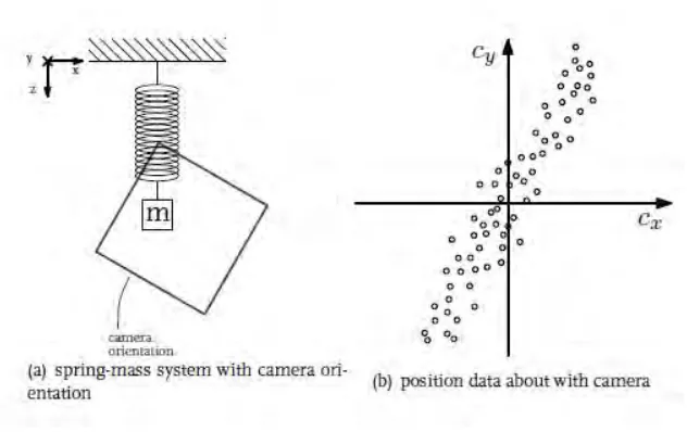
To illustrate the basic ideas of PCA, an example of a spring-mass system shown in figure is used throughout this section. By moving the mass down, outside its equilibrium position and letting go, the mass should translate continuously up and down assuming no friction forces. The movement of the mass is our main interest and we try to analyze this by capturing its movement using a camera.

Of course we know that the line of action is along the z-axis, but we pretend we do not have any information about the system a priori. Therefore we position the camera arbitrarily in a plane parallel to the mass. The slightly tilted camera captures the position of the mass with a certain sampling frequency and a possible data set of a measurement with this configuration is shown in figure 2.1.1(b). Here the circles represent the position of the mass during the measurement.

Basically the goal of PCA is to clarify the data by re-expressing the data by means of a new coordinate basis. Now consider an [e × t] original data matrix E, where e is the number of dimensions measured and t represents the number of time samples taken. The matrix E can be converted to a new representation of the data, C, by an [e × e] transformation matrix T;

C = TE (2.2)