Thesis by
Kevin Kaichuang Yang
In Partial Fulfillment of the Requirements for the Degree of
Doctor of Philosophy in Chemical Engineering
CALIFORNIA INSTITUTE OF TECHNOLOGY Pasadena, California
2019
© 2019
Kevin Kaichuang Yang ORCID: 0000-0001-9045-6826
ACKNOWLEDGEMENTS
First, I’d like to thank my advisor Frances Arnold for her support and guidance throughout my PhD. I applied to Caltech because I wanted to work for Frances, and she has not disappointed. Even as I took a detour to teach high school, she welcomed me into her lab first for a summer, and then for my PhD. Frances has a keen eye for important but tractable scientific problems and gave me the freedom to pursue them past the boundaries of her discipline. Frances has pushed me to be a better scientist, and her lessons are the foundation for the rest of my career.
One thing Frances has done very well is to build a world-class research group. I would like to specifically thank several group members. During my first stint in the lab, Sabine Brinkmann-Chen, John McIntosh, and Chris Farwell taught me to perform directed evolution. Sabine also keeps us all safe, happy, and productive. When I rejoined the lab, Lukas Herwig reacquainted me with molecular biology. It was a joy to work with Claire Bedbrook and Austin Rice on my first three papers. Thank you for collecting my data for me. Zachary Wu has been a great co-belligerent for the cause of machine learning in the Arnold lab. Thank you for the discussions and advice. Finally, I’d like to thank the two undergraduate researchers who worked with me: Raul Sun Han and Alycia Lee. I hope my mentorship was a fair trade for all the work you did. Philip Romero now leads his own group, but I am indebted to him for starting the machine learning work in the Arnold lab, providing me with his code and data, and being on my candidacy committee.
Almost all of my formal training in machine learning comes from Yisong Yue. Yisong taught me the foundations of machine learning and pointed the way towards successful applications to proteins. Most importantly, he has shown me how to be a machine learning researcher. I was also fortunate to collaborate with Yisong’s postdoc Yuxin Chen. Thank you for your patience as I learned new fields and for your good humor through the late nights. Without Yisong’s guidance and Yuxin’s hands-on help, I would still be stumbling in the dark.
running and answer all my questions, and my classmates Bradley Silverman and Heidi Klumpe, who helped me pass my classes and quals and have been great friends over the last 4 years.
Outside of chemical engineering, Justin Bois and Kimberly Mayer have both made significant contributions to my development as a scientist. Justin is my role model in computational science and thoughtful teaching. Kimberly has been invaluable in helping me navigate grant-writing, communication, and science careers.
ABSTRACT
PUBLISHED CONTENT AND CONTRIBUTIONS
1. Kevin K Yang, Zachary Wu, and Frances H Arnold: Machine learning in protein engineering (2018). eprint: https://arxiv.org/abs/1811.10775.
K.K.Y. participated in the conception of the project and wrote the manuscript. 2. Kevin Yang, Zachary Wu, Claire Bedbrook, and Frances Arnold: Learned Protein
Embeddings for Machine Learning.Bioinformatics(2018). doi: 10.1093/bioinformatics/bty178.
K.K.Y conceived the project, built and trained machine-learning models, prepared the data, and wrote the manuscript.
3. Claire N Bedbrook, Kevin K Yang, Austin J Rice, Viviana Gradinaru, and Frances H Arnold: Machine learning to design integral membrane
channelrhodopsins for efficient eukaryotic expression and plasma membrane localization.PLoS Computational Biology13(10) (2017), e1005786. doi: 10.1371/journal.pcbi.1005786.
K.K.Y. participated in the conception of the project, built and trained machine-learning models, and participated in the writing of the manuscript. 4. Claire N Bedbrook, Kevin K Yang, J Elliot Robinson, Viviana Gradinaru, and
Frances H Arnold: Machine learning-guided channelrhodopsin engineering enables minimally-invasive optogenetics (Submitted).
TABLE OF CONTENTS
Acknowledgements . . . iii
Abstract . . . v
Published Content and Contributions . . . vi
Table of Contents . . . vii
List of Illustrations . . . ix
List of Tables . . . xxvi
Chapter I: Machine learning for protein engineering . . . 1
1.1 Introduction . . . 1
1.2 A brief introduction to machine learning on proteins . . . 3
1.3 Machine learning as a guide to directed evolution . . . 12
1.4 Conclusions and future directions . . . 15
Chapter II: Machine learning to design integral membrane channelrhodopsins for efficient eukaryotic expression and plasma membrane localization . . . 28
2.1 Introduction . . . 28
2.2 Results . . . 30
2.3 Discussion . . . 44
Chapter III: Machine learning-guided channelrhodopsin engineering enables minimally-invasive optogenetics . . . 66
3.1 Introduction . . . 66
3.2 Results . . . 67
3.3 Discussion . . . 80
Chapter IV: Learned protein embeddings for machine learning . . . 98
4.1 Introduction . . . 98
4.2 Methods . . . 102
4.3 Results and Discussion . . . 105
4.4 Conclusions . . . 111
Chapter V: Batched Stochastic Bayesian Optimization via Combinatorial Constraints Design . . . 119
5.1 Introduction . . . 119
5.2 Related Work . . . 120
5.3 Problem Statement . . . 122
5.4 Algorithms . . . 124
5.5 Experiments . . . 128
5.6 Conclusion . . . 133
Chapter VI: Learned decomposition kernels for sequence-function prediction 141 6.1 Introduction . . . 141
6.2 Gaussian processes . . . 142
6.3 Related work . . . 143
LIST OF ILLUSTRATIONS
Number Page
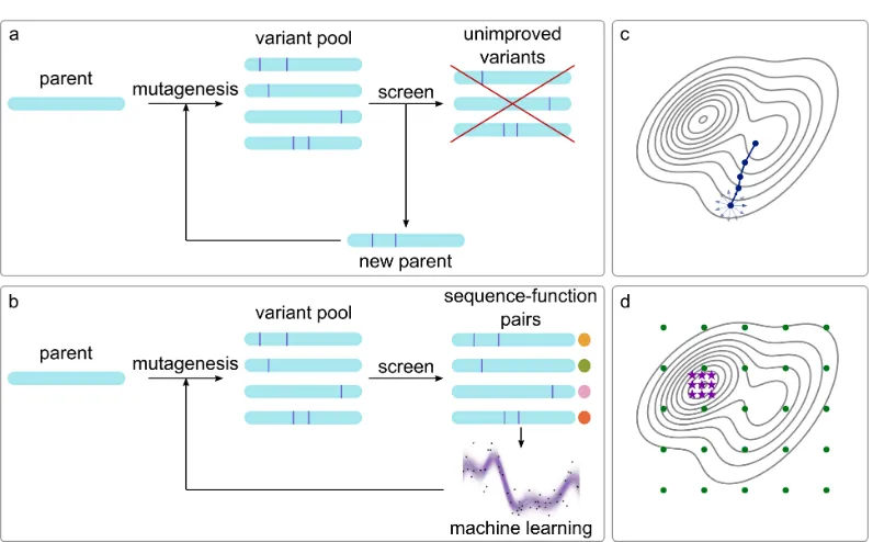
1.1 Directed evolution with and without machine learning. (a) Directed evolution uses iterative cycles of diversity generation and screening to find improved variants. Information from unimproved variants is discarded. (b) Machine-learning methods use the data collected in each round of directed evolution to choose the mutations to test in the next round. Careful choice of mutations to test decreases the screening burden and improves outcomes. (c) Directed evolution is a series of local searches on the fitness landscape. (d) Machine learning-guided directed evolution often rationally chooses the initial points (green circles) to maximize the information learned from the fitness landscape, allowing future iterations to quickly converge to improved sequences (violet stars). . . 3 1.2 Examples of model interpretation. (a) Local approximation. The
1.3 Gaussian Process Upper Confidence Bound algorithm. At each it-eration, the next point to be sampled is chosen by maximizing the weighted sum of the posterior mean and standard deviation. This balances exploration and exploitation by exploring points that are both uncertain and have a high posterior mean. . . 15 1.4 Autoencoder. An autoencoder consists of an encoder model and a
decoder model. The encoder converts the input to a low-dimensional vector (code). The decoder reconstructs the input from this code. Typically, the encoder and decoder are both neural network models, and the entire autoencoder model is trained end-to-end. The learned code should contain sufficient information to reconstruct the inputs and can be used as input to other machine learning methods, or the autoencoder itself may be used as a generative model. . . 17 2.1 General approach to machine learning of protein (ChR)
2.2 GP binary classification models for expression and localization. Plots of predicted probability vs measured properties are divided into ‘high’ performers (white background) and ‘low’ performers (gray back-ground) for each property (expression and localization). (A) & (D) Predicted probability vs measured properties for the training set (gray points) and the exploration set (cyan points). Predictions for the train-ing and exploration sets were made ustrain-ing LOO cross-validation. (B) & (E) Predicted probabilities vs measured properties for the verifi-cation set. Predictions for the verifiverifi-cation set were made by a model trained on the training and exploration sets. (C) & (F) Predicted prob-ability of ‘high’ expression, and localization for all chimeras in the recombination library (118,098 chimeras) made by models trained on the data from the training and exploration sets. The gray line shows all chimeras in the library, the gray points indicate the training set, the cyan points indicate the exploration set, the purple points indi-cate the verification set, and the yellow points indiindi-cate the parents. (A–C) Show expression and (D–F) show localization. For all plots, the measured property is plotted on a log2scale. . . 37 2.3 Comparison of measured membrane localization for each data set.
2.4 GP regression model for localization. (A) Predicted vs measured localization for the combined training and exploration sets (gray points), verification set (purple points), and the optimal set (green points). Predictions for the training and exploration sets were made using LOO cross-validation; predictions for the verification and op-timal sets were made by a model trained on data from the training and exploration sets. There is clear correlation between predicted and measured localization. The combined training and exploration sets showed good correlation (R > 0.73) as did the verification set (R > 0.9). (B) Predicted localization values of all chimeras in the recombination library (118,098 chimeras) based on the GP regres-sion model trained on the training and exploration sets. The gray line shows all chimeras in the library, the gray points indicate the training set and exploration sets, the purple points indicate the verification set, and the yellow points indicate the parents. Error bars (light gray shading) show the standard deviation of the predictions. For all plots, the predicted and measured localization are plotted on a log2scale. . 40 2.5 Sequence and structural contact features important for prediction of
2.6 GP regression model enables engineering of localization in CbChR1. (A) Block identities of the CsCbChR1 chimeras. Each row represents a chimera. Yellow represents the CbChR1 parent and red represents the CsChrimR parent. Chimeras 1c, 2n, and 3c have 4, 21, and 17 mu-tations with respect to CsCbChR1, respectively. (B) Plot of measured localization of CsCbChR1 compared to three CsCbChR1 single-block-swap chimeras and the CheRiff parent. (C) Two representative cell images of mKate expression of CbChR1 and CsCbChR1 com-pared with top-performing CsCbChR1 single-block-swap chimeras show differences in ChR localization properties–chimera 2n and chimera 3c clearly localize to the plasma membrane. Scale bar: 20 µm. . . 44 2.S1 Chimera sequences in training set and their expression, localization,
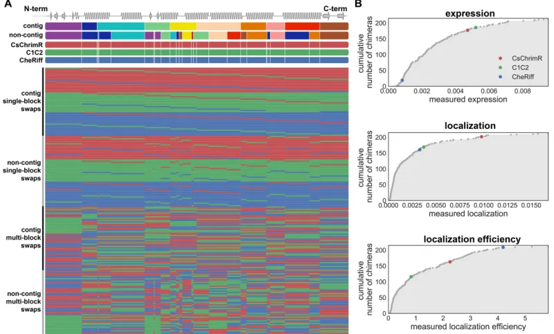
and localization efficiencies. (A) (top) shows blocks (different colors) for the contiguous (contig) and non-contiguous (non-contig) library designs and also shows block boundaries (white lines) for the com-bined contiguous and non-contiguous library designs on the three parental ChRs aligned with a schematic of the ChR secondary struc-ture. (bottom) Sequences of training set chimeras showing block identities. The colors represent the parental origin of the block (red–CsChrimR, green–C1C2, and blue–CheRiff). (B) Cumulative distributions of the measured expression, localization, and localiza-tion efficiency of all 218 chimeras with the three parental constructs highlighted in color (5). . . 54 2.S2 Chimera expression and localization cannot be predicted from
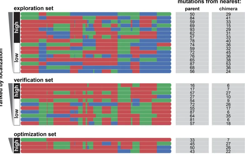
2.S3 GP binary classification model for localization efficiency. Plots of predicted probability vs measured localization efficiency are divided into ‘high’ performers (white background) and ‘low’ performers (gray background) for localization efficiency. (A) Predicted probability vs measured localization efficiency for the training set (gray points) and the exploration set (cyan points). Predictions for the training and exploration sets were made using LOO cross-validation. (B) Predicted probabilities vs measured localization efficiency for the verification set. Predictions for the verification set were made by a model trained on the training and exploration sets. (C) Probability of ‘high’ localization efficiency for all chimeras in the recombination library (118,098 chimeras) made by a model trained on the data from the training and exploration sets. The gray line shows all chimeras in the library, the gray points indicate the training set, the cyan points indicate the exploration set, the purple points indicate the verification set, and the yellow points indicate the parents. For all plots, the measured localization efficiency is plotted on a log2scale. . . 56 2.S4 Chimera block identities for exploration, verification, and
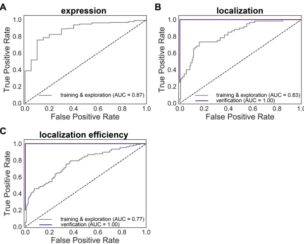
2.S5 ROC curves for GP classification expression, localization, and lo-calization efficiency models. ROC curves show true positive rate vs false positive rate for predictions from the expression (A), localiza-tion (B), and localizalocaliza-tion efficiency (C) classificalocaliza-tion models. The gray line shows the ROC for the combined training and exploration sets. The purple line shows the ROC for the verification set. The ver-ification sets consist exclusively of chimeras with ‘high’ expression so no verification ROC curve for expression is shown. Predictions for the training and exploration sets were made using LOO cross-validation, while predictions for the verification set were made by a model trained on the training and exploration sets. Calculated AUC values are shown in the figure key. . . 58 2.S6 Comparison of measured expression and localization efficiency for
each data set. Swarm plots of expression (A) and localization effi-ciency (B) measurements for each data set compared with parents: training set, exploration set, verification set, and optimization set. . . 59 2.S7 Cell population distributions of expression, localization, and
2.S8 Predictive ability of GP localization models as a function of training set size.We trained GP models on random training sets of various sizes sampled from our data and evaluated their predictive perfor-mance on a fixed test set of sequences for the classification (A) and regression (B) localization models. The predictive performance of the classification model is described by AUC for the test set (A), while the predictive performance of the regression model (B) is de-scribed by the correlation coefficient (R-value) for the test set. For each training set size, the results are averaged over 100 random samples. 61 2.S9 Important features for prediction of ChR localization aligned with
chimeras with optimal localization. Features with positive weights from the localization model (Figure 2.5) are displayed on the C1C2 crystal structure which is colored based on the block design of two different chimeras, (A) n1_7 and (B) n4_7, from the optimization set. Features can be residues (spheres) or contacts (sticks) from one or more parent ChRs. Features/blocks from CsChrimR are shown in red, features/blocks from C1C2 are shown in green, and fea-tures/blocks from CheRiff are shown in blue. Gray positions are conserved residues. Sticks connect the beta carbons of contacting residues (or alpha carbon in the case of glycine). The size of the spheres and the thickness of the sticks are proportional to the param-eter weights. . . 62 2.S10 GP regression model for ChR expression. Shows the GP regression
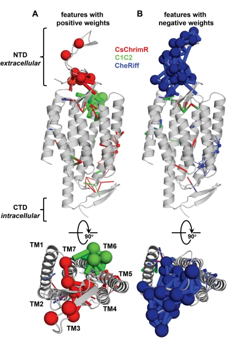
2.S11 Sequence and structure features important for prediction of ChR expression. Features with positive (A) and negative (B) weights are displayed on the C1C2 crystal structure (grey). Features can be residues (spheres) or contacts (sticks) from one or more parent ChRs. Features from CsChrimR are shown in red, features from C1C2 are shown in green, and features from CheRiff are shown in blue. In cases where a feature is present in two parents, the following color priorities were used for consistency: red above green above blue. Sticks connect the beta carbons of contacting residues (or alpha carbon in the case of glycine). The size of the spheres and the thickness of the sticks are proportional to the parameter weights. Two residues in contact can be from the same or different parents. Single-color contacts occur when both contributing residues are from the same parent. Multi-color contacts occur when residues from different parents are in contact. The N-terminal domain (NTD), C-terminal domain (CTD), and the seven transmembrane helices (TM1-7) are labeled. . . 64 2.S12 Localization of engineered CbChR1 variant chimera 3c.
3.1 Machine learning-guided optimization of ChR photocurrent strength, off-kinetics, and wavelength sensitivity of activation. (a) Upon light exposure, ChRs rapidly open and reach a peak inward current; with continuous light exposure, ChRs desensitize reaching a lower steady-state current. Both peak and steady-state current are used as metrics for photocurrent strength. To evaluate ChR off-kinetics, the current decay after a 1 ms light exposure is fit to a monoexponential decay curve and the decay rate (τoff) is used
3.2 Training machine-learning models to predict ChR properties of interest based on sequence and structure enables design of ChR variants with col-lections of desirable properties. (a) Measurements of training set ChR and model-predicted ChR, peak photocurrent, off-kinetics, and normalized green current. Each gray-colored point is a ChR variant. Training set data are shaded in blue. Mean number of mutations for each set is above the plots. (b) Model predictions vs measured property for peak photocurrent, off-kinetics, and normalized green current of the 28 designer ChRs shows strong correlation. Specific ChR variants are highlighted to show predicted and measured properties for all three models: blue, ChR_12_10, green, ChR_11_10, orange, ChR_28_10, pink, ChR_5_10. . . 72 3.3 The model-predicted ChRs exhibit a large range of functional properties
of-ten far exceeding the parents. (a) Current trace after 0.5 s light exposure for select designer ChR variants with corresponding expression and localization in HEK cells. Vertical colored scale bar for each ChR current trace repre-sents 0.5 nA, and horizontal scale bar reprerepre-sents 250 ms. Different color traces are labeled with each variant’s name. The variant color presented in (a) is kept constant for all other panels. (b) Designer ChR measured peak and steady-state photocurrent with different wavelengths of light. 383 nm light at 1.5 mW mm−2, 485 nm light at 2.3 mW mm−2, 560 nm light at 2.8 mW mm−2, and 650 nm light at 2.2 mW mm−2. (c) Designer ChR off-kinetics decay rate (τoff) following a 1 ms exposure to 485 nm light (2.3
3.5 Validation of high conductance hi-ChR2 for minimally-invasive optoge-netic behavioral modulation. (a) Minimally-invasive, systemic delivery of rAAV-PHP.eB packaged CAG-DIO hi-ChR2-TS-eYFP or ChR2(H134R)-TS-eYFP (3 ×10¹¹ vg/mouse) into Dat-Cre animals coupled with fiber optic implantation above the VTA enabled blue light-induced intracranial self-stimulation (ten 5 ms laser pulses) exclusively with hi-ChR2 and not ChR2(H134R) with varying light power and varying stimulation frequen-cies. hi-ChR2, n = 4; ChR2(H134R), n = 4. (b) Minimally-invasive, systemic delivery of rAAV-PHP.eB packaged CaMKIIa hi-ChR2-TS-eYFP or ChR2(H134R)-TS-eYFP (5×10¹¹vg/mouse) into wild type (WT) ani-mals coupled with surgically secured 2 mm long, 400µm fiber-optic cannula guide to the surface of the skull above the right M2 that had been thinned to create a level surface for the fiber-skull interface. Three weeks later, mice were trained to walk on a linear-track treadmill at fixed velocity. Unilateral blue light stimulation of M2 induced turning behavior exclusively with hi-ChR2 and not hi-ChR2(H134R) (10 Hz stimulation with 5 ms 447 nm light pulses at 20 mW). hi-ChR2, n = 5; ChR2(H134R), n = 5. No turning behavior was observed in any animal with 10 Hz stimulation with 5 ms 671 nm light pulses (20 mW). Error bars represent standard error of the mean. vg, viral genomes. . . 81 3.S1 Thirty model-predicted ChR chimeras aligned with the three parents
and the secondary structure. Blocks of ChR chimeras are colored according to which parent each block came from. CsChrimR is red, CheRiff is blue, and C1C2 is green. (*) highlights the Schiff base. ChRs are divided into categories based on their predicted properties. Twenty-eight ChR chimeras are predicted to be optimized for one or more properties. Two ChR chimeras are predicted to be non-optimal and produce low currents. A number of chimeras appear twice because they were optimal for multiple categories. . . 93 3.S2 Specific residues (amino-acid sticks) and contacts (dark gray lines)
most important for model prediction of off-kinetics and photocurrent strength overlaid on the C1C2 crystal structure in light gray (3ug9.pdb). 94 3.S3 Specific residues (amino-acid sticks) and contacts (dark gray lines)
3.S4 HEK cell expression of selected high-conductance ChR variants. Plot of measured expression in HEK cells for each variant (CheRiff,n=17 cells; C1C2, n = 14 cells; CsChrimR, n = 12 cells; ChR_10_10,
n = 5 cells; ChR_11_10, n = 15 cells; ChR_12_10, n = 11 cells; ChR_9_4, n = 9 cells; ChR_25_9, n = 11 cells). Plotted data are mean± SEM. No significant difference between CsChrimR and the high-conductance ChR variants with ANOVA and Dunnett’spost hoc
test. . . 95 3.S5 (a) Construct design for each ChR tested with a trafficking sequence,
eYFP, and WPRE under the hSyn promoter. (b) Peak and steady-state photocurrent comparison between high-conductance ChRs, ChR2(H134R), and CoChR with both high-intensity and low-intensity light. Mul-tiple HEK cells were recorded from for each ChR: ChR2(H134R),
n= 11 cells; CoChR, n= 7 cells; 11_10,n = 9 cells; 25_9, n= 12 cells; 9_4, n = 9 cells. Plotted data are mean ± SEM. There is a significant difference between the high-conductance ChR variants and ChR2 with low intensity light (P < 0.0001 for 11_10, 25_9, and 9_4); ANOVA and Dunnett’spost hoctest, with ChR2 as a reference. There is a significant difference between the high-conductance ChR variants and CoChR with low intensity light (P = 0.007 for 11_10,
P < 0.003 for 25_9, andP < 0.0005 for 9_4); ANOVA and Dunnett’s
post hoctest, with CoChR as a reference. . . 96 3.S6 Top five high-conductance ChRs predicted by the machine-learning
4.1 The modeling scheme. First, an unsupervised embedding model is trained on 524,529 unlabeled sequences pulled from the UniProt database. The UniProt sequences are broken into k lists of non-overlapping k-mers (Step 1), and then the lists are used to train the embedding model (Step 2). The doc2vec embed-ding model learns to predict the vectors for center k-mers from the vectors for their sur-rounding context k-mers and the sequence vectors. These sequence vectors are then the embedded representations of the sequences. Next, information learned during the unsupervised phase is applied during supervised learning with labeled sequences. The labeled sequences for each task (localiza-tion, T50, absorption, and enantioselectiv-ity) are first broken into k lists of non-overlapping k-mers (Step 3). An embedding is then inferred for each se-quence using the trained embedding model (Step 4). n is the number of labeled sequences. Finally, during GP regression (Step 5), the inferred training embed-dings X0and the training labels y are used to train a GP regression model, which can then be used to make predictions. . . 101 4.2 Effect of embedding dimension on predictive accuracy. For each
task, embeddings of varying dimensions were trained and then used for GP regression. The resulting model quality was then evaluated using the Kendall’sτand MAE. . . 109 4.3 Effect of number of unlabeled sequences on predictive accuracy.
For each task, embeddings were trained on subsets of the UniProt sequences and then used for GP regression. The resulting model quality was then evaluated using the Kendall’sτand MAE. . . 109 4.4 Visualization of learned vector representations of protein sequences.
Vector representations projected onto 2 dimensions using t-SNE with perplexity 50 (embeddings, AAIndex, sequence) or 10 (ProFET). The sequences for the localization, the T50 and the enantioselectivity tasks are colored by the number of mutations from the nearest parent. The sequences for the absorption task are colored by peak absorption wavelength. Parents for localization, T50 and enantioselectivity are indicated by red triangles. . . 110 4.5 Combined visualization of vector representations for each of the four
4.S1 Test predictions for ChR localization. Predicted vs measured values on test sequences using GP regression models trained using each encoding method. . . 114 4.S2 Test predictions for P450 T50. Predicted vs measured values on test
sequences using GP regression models trained using each encoding method. . . 114 4.S3 Test predictions for rhodopsin absorption. Predicted vs measured
values on test sequences using GP regression models trained using each encoding method. . . 115 4.S4 Test predictions for epoxide hydrolase enantioselectivity. Predicted
vs measured values on test sequences using GP regression models trained using each encoding method. . . 116 4.S5 t-SNE visualizations calculated for all embeddings. Visualizations
for localization and T50 are colored according to the closest recombi-nation parent. Visualizations for absorption are colored according to whether the peak absorption wavelength is blue- or red-shifted com-pared to the parent. Visualizations for enantioselectivity are colored by whether each sequence is above or below the median (e = 46). . . 116 5.1 Data-driven site-saturation mutagenesis. (1) Machine learning model
for predicting certain protein properties ; (2) site-saturation library de-sign; (3) synthesize protein sequences according to the site-saturation libraries; (4) randomly sample proteins for sequencing; (5) sequence and measure the properties of the sampled proteins. . . 120 5.2 The batched stochastic Bayesian optimization setting. (1) Bayesian
modeling (2) combinatorial constraints design; (3) candidate query generation; (4) random sampling; (5) batched queries. . . 123 5.3 The cell values for the synthetic dataset with L = 2 and |C(`)| =
26∀` ∈ {1,2}. . . 129 5.4 Performance of each algorithm on finding constraints on synthetic
datasets. Error bars are standard errors. ˆF is the approximate objec-tive, andnis the batch size. . . 130 5.5 Comparing ˆF (Eq. (5.2)) against the Monte Carlo estimates of F
5.6 Results on (a) GB1 and (b) PhoQ when runningOnline-DSOptwith different batch sizes, with a total budget of 400 samples. In the left plots, each colored line corresponds to a different batch size, and every marker corresponds to the maximal value of f found at the end of that batch. The solid horizontal lines show the fitnesses for the wild-type sequences (wt) as the baseline of the batched experiments. The dashed horizontal lines show the fitnesses for the best sequences with exactly one mutation from the wild type (single). The dotted horizontal lines show the fitnesses for the sequences that combine the best amino acid at each site determined in the wild-type background (recombine). The plots on the right show the probability mass of each fitness value in the corresponding dataset. . . 132 5.7 Fitness values f for the sampled protein sequences when running
Online-DSOpt over four rounds. Each round contains 100 samples
(n = 100). Different rounds are represented with different colors, and each point represents a protein sequence sampled in the corre-sponding round. . . 133 6.1 Example of a learned decomposition kernel between two sequences
LIST OF TABLES
Number Page
1.1 Comparison of selected studies using machine learning to guide di-rected evolution . . . 15 2.1 Comparison of size, diversity, and localization properties of the
train-ing set and subsequent sets of chimeras chosen by models in the iterative steps of model development . . . 32 3.1 Evaluation of prediction accuracy for different ChR property models.
Calculated AUC or Pearson correlation after 20-fold cross validation on training set data for classification and regression models. The test set for both the classification and regression models was the 28 ChR sequences predicted to have useful combinations of diverse properties. Accuracy of model predictions on the test set is evaluated by AUC (for classification model) or Pearson correlation (for the regression models). The Matérn kernel is withν = 52. . . 71 3.S1 List of different constructs made for validation of the high-conductance
ChRs. . . 97 3.S2 GP regression model hyperparameters for each ChR property of
in-terest for the Matérn kernel. . . 97 4.1 Summary of tasks used to evaluate embedded representations . . . . 105 4.2 Comparison of learned, dense, embedded representations, ProFET,
C h a p t e r 1
MACHINE LEARNING FOR PROTEIN ENGINEERING
1. Kevin K Yang, Zachary Wu, and Frances H Arnold: Machine learning in protein engineering (2018). eprint: https://arxiv.org/abs/1811.10775.
1.1 Introduction
Protein engineering seeks to design or discover proteins whose properties, useful for technological, scientific, or medical applications, have not been needed or optimized in nature. We can envision the mapping of protein sequence to a desired function or functions as a “fitness landscape” over the high-dimensional space of possible protein sequences1. The fitness represents a protein’s performance: expression level, catalytic activity, or other properties of interest to the protein engineer. The landscape determines the range of properties available to different sequences as well as the ease with which they can be optimized. In one limit, convex landscapes that climb smoothly to a global maximum are easy to search. In the other, rugged landscapes with many local maxima are much more difficult to traverse. Protein engineering seeks to identify sequences corresponding to high fitnesses on these landscapes.
Identifying optimal locations on a fitness landscape is extremely challenging. The space of possible protein sequences is too large to be searched exhaustively naturally, in the laboratory, or computationally2. The problem of finding optimal sequences is NP-hard, meaning that there is no known polynomial-time method for searching this space3. Functional proteins are also extremely scarce in this vast space of sequences. Moreover, as the threshold level of fitness increases, the number of sequences having that fitness decreases exponentially4,5. As a result, highly fit sequences are vanishingly rare and overwhelmed by nonfunctional and mediocre sequences.
sequences that fold into desired static structures8. This is an important advance, and useful when a single stable structure dictates function8. However, because proteins are marginally stable, even small inaccuracies in energy-based scoring functions can lead to very poor performance9.
Many protein functions such as binding, catalysis, allostery, and signalling, are mediated through recessed cavities, mobility, or multiple low-energy states10. For example, computational enzyme design currently proceeds by designing an idealized active site for the desired reaction, matching the active site residues to stable back-bones, and then using molecular dynamics (MD) simulations to winnow designs with flaws not apparent from static evaluations. MD simulations require enormous computational resources (100s of CPU hours for each variant) and are not appropri-ate for testing many variants. This process generally yields sequences with modest activity that are finally improved with directed evolution11.
Inspired by natural evolution, directed evolution climbs a fitness landscape by accu-mulating beneficial mutations in an iterative protocol of mutation and selection, as illustrated in Figure 1.1a. The first step is sequence diversification using techniques such as random mutagenesis, site-saturation mutagenesis, or recombination to gen-erate a library of modified sequences starting from the parent sequence(s). The second step is screening or selection to identify variants with improved properties for the next round of diversification. The steps are repeated until fitness goals are achieved.
Directed evolution is limited by the fact that even the most high-throughput screen-ing or selection methods only sample an insignificant fraction of the sequences that can be made using most diversification methods, and developing efficient screens is nontrivial. Moreover, directed evolution requires at least one minimally-functional parent and a locally-smooth fitness landscape for stepwise optimization1. Recom-bination methods may allow for bigger jumps in sequence space while retaining function12, but sequences designed using recombination are by definition restricted to exploring combinations of previously-explored mutations. No matter the diversi-fication technique, directed evolution is energy-, time-, and material-intensive, and multiple generations of evolution may be required to achieve meaningful perfor-mance improvements.
Figure 1.1: Directed evolution with and without machine learning. (a) Directed evolution uses iterative cycles of diversity generation and screening to find improved variants. Information from unimproved variants is discarded. (b) Machine-learning methods use the data collected in each round of directed evolution to choose the mutations to test in the next round. Careful choice of mutations to test decreases the screening burden and improves outcomes. (c) Directed evolution is a series of local searches on the fitness landscape. (d) Machine learning-guided directed evolution often rationally chooses the initial points (green circles) to maximize the information learned from the fitness landscape, allowing future iterations to quickly converge to improved sequences (violet stars).
function can be predictive even when the underlying mechanisms are not well-understood. As shown in Figure 1.1b, machine-learning models can guide directed evolution by learning from the information contained in all measured variants. This new paradigm for protein engineering enables engineering with fewer measurements and fewer generations of evolution. Here, we cover the basics of machine learning with a focus on applications to protein engineering and protein sequence-function datasets, discuss how machine learning can be integrated with directed evolution to accelerate protein engineering, and consider the developments that are required to enable wider applications.
1.2 A brief introduction to machine learning on proteins
contrast, machine-learning models infer patterns from data, which can then be used to make predictions on unobserved data. The user must collect the training data, represent it in a form amenable to machine learning, decide what type of machine-learning algorithm to use, and train and interpret the model.
Protein function databases
The broadest protein datasets are UniProt, which aims to catalog all known protein sequences15, the Protein Data Bank16, which catalogs all known protein struc-tures, and BRENDA, which catalogs natural enzymes and their functions17. These databases do not specifically store sequence-function relationships.
Protein engineering experiments have generated a growing collection of well-characterized libraries. Databases that collect and organize specific categories of sequence-function data include ProTherm and ProNit for protein stability and protein-nucleic acid interactions, respectively18, and SKEMPI19, AB-Bind20, and PROXIMATE21for protein-protein complexes. The Protein Mutant Database22, an early attempt to catalog the effects of mutations from protein engineering studies across different proteins and functions, has not been updated in over a decade. Cur-rently, Protabank is an actively-maintained and updated database for general protein design and engineering data23.
ProTherm is the oldest and most mature of these databases, but has not been updated since 2013. There have been many efforts to use the sequence-function information in ProTherm to train machine-learning models to predict the effects of mutations on stability24–35. However, Yanget al. found that ProTherm contains many errors and cautions against using entries as training sets without proper validation36.
Vector representations of proteins
For machine-learning models to learn about protein sequences, protein sequences must be represented as vectors or matrices of numbers. How each protein sequence is represented determines what can be learned37,38. Even the most powerful models produce poor results if an inappropriate representation is used. An ideal encoding would perform well across different proteins and functions, not require alignments, structures, or feature selection, and transfer the information contained in unlabeled sequences to specific prediction tasks. Unfortunately, such an encoding does not exist.
for a particular task. Most representations using physical properties also require alignments of the input sequences.
AAIndex42 attempts to systematically collect descriptors of protein sequences. AAIndex comprises three sections: AAIndex1 contains 554 amino acid features, AAIndex2 contains 94 amino acid substitution matrices, and AAIndex3 contains 47 amino acid contact potential matrices. ProFET is another encoding system that considers physical properties of the bulk protein, the individual residues, and sub-sequences of residues43. There have also been attempts to describe each amino acid using two reduced dimensions based on volume and hydrophobicity44 and to com-bine physical properties with structural information30,45 by encoding each position in the sequence as a combination of the properties of amino acids in its geometric neighborhood.
While there are a vast number of known protein sequences, only a tiny fraction are labeled with measured properties relevant to any specific prediction task. The number of unlabeled sequences will continue to rise as more sequences are deposited into public databases. These unlabeled sequences contain information about the frequency and patterns of amino acids selected by evolution to compose proteins, information that may be helpful across prediction tasks. The simplest examples are BLOSUM46 or AAIndex2-style substitution matrices based on relative amino-acid frequencies. However, more sophisticated continuous vector encodings of sequences can be learned from patterns in unlabeled sequences47–52. These representations are known as embedded representations. Conceptually, through sequence context, these representations learn a mapping from a space with one indicator (one-hot) dimension per k-mer or protein sequence to a continuous vector space with a much lower dimension such that similar sequences are close together in the continuous space. When modeling large (> 104 examples) datasets with neural networks, embeddings for individual amino acids or k-mers can be learned simultaneously with the model weights. Learned encodings are low-dimensional, do not require alignments, and may improve performance by transferring information in unlabeled sequences to specific prediction tasks. However, it is difficult to predict which learned encoding will perform well for any given task.
performance to general sets of protein properties51, although careful feature selection informed by domain knowledge may yield more accurate predictions. If accuracy is insufficient, learned encodings may be able to improve performance. The encoding should ultimately be chosen empirically to maximize predictive performance.
Models for protein data
A wide range of machine-learning algorithms exist, and no single algorithm is opti-mal across all learning tasks53. Machine-learning methods can be broadly classified as supervised, unsupervised, or semi-supervised. In supervised learning, the train-ing data consist of inputs and their associated output values (labels). Supervised methods learn a mapping from input space to output space that enables them to accurately predict outputs from new inputs. Supervised learning can be further di-vided into regression, which aims to predict real-valued outputs, and classification, which aims to predict class membership. In unsupervised learning, the training data consist only of input values. Unsupervised methods learn to find patterns, such as trends or clustering, in the inputs. In semi-supervised learning, the training data consist of inputs, of which a subset has associated output values. Semi-supervised methods leverage information in the unlabeled training inputs to improve their abil-ity to predict outputs from inputs. Supervised learning is the most developed of these approaches, and is used in the majority of applications to protein engineering. We outline some common supervised machine-learning algorithms below.
The simplest machine-learning models apply a linear transformation of the input features, such as the amino acid at each position, the presence or absence of a mutation54, or blocks of sequence in a library of chimeric proteins made by re-combination55. Linear models are simple and the learned parameters are easily interpreted by the user. Linear models are commonly used as baseline predictors before more powerful models are tried.
Classification and regression trees56 use a decision tree to go from input features (represented as branches) to labels (represented as leaves). Decision tree models are often used in ensemble methods, such as random forests57or boosted trees58, which combine multiple models into a more accurate meta-predictor. For small biological datasets (< 104 training examples), including those often encountered in protein engineering experiments, random forests are a strong and computationally efficient baseline, and have been used to predict thermostability24–26.
employ a kernel function, which calculates similarities between pairs of inputs, to implicitly project the input features into a high-dimensional feature space without explicitly calculating the coordinates in this new space. The choice of kernel profoundly affects the accuracy of these methods. While general-purpose kernels can be applied to protein inputs, there are also kernels designed for use on proteins, including spectrum and mismatch string kernels61,62, which count the number of shared sub-sequences between two proteins, and weighted decomposition kernels33 and other graph kernels, which account for three-dimensional protein structure. Support vector machines have been used to predict protein thermostability24–31, enantioselectivity63, and membrane protein expression64.
Gaussian process regression and classification combine kernel methods with Bayesian learning to produce probabilistic predictions65. These models rigorously capture uncertainty, which, combined with methods from Bayesian optimization, can pro-vide principled ways to guide experimental design in optimizing protein properties. The run-time for exact GP regression scales as the number of training examples cubed, making it unsuitable for large (> 103) datasets, but there are now fast and accurate approximations66. Gaussian processes have been used to predict ther-mostability32,33,39, enzyme substrates67, fluorescence68, membrane localization40, and channelrhodopsin photo-properties69.
Deep learning models, also known as neural networks, stack multiple linear layers connected by non-linear activation functions, allowing them to extract high-level features from structured inputs. Neural networks are well-suited for tasks with large labeled datasets with examples from many protein families, such as protein-nucleic acid binding70–72, protein-MHC binding73, binding site prediction74, protein-ligand binding48,75, solubility76, thermostability34,35, subcellular localization77, secondary structure78, functional class79,80, and even 3D structure81. Deep learning networks are also particularly useful in metabolic pathway optimization82and genome anno-tation83–85, which have been reviewed elsewhere.
k-nearest-neighbor86 methods make predictions on new data points by taking the majority (for classification) or mean (for regression) labels for theknearest training points. The quality of the predictions can be affected by setting the neighborhood size
computationally expensive,k-nearest-neighbor methods are not commonly applied to protein datasets.
Model training and evaluation
All model families have hyperparameters that determine the form of the model. Unlike model parameters, hyperparameters cannot be learned directly from the data. These may be set manually by the practitioner or determined using a procedure such as grid search, simulated annealing, random search, or Bayesian optimization. Hyperparameters may be discrete or continuous. For example, in support vector machines, the type of kernel is a hyperparameter, as are the number of layers and learning rate in a deep neural network. The vectorization method is also a hyperparameter. Even modest changes in the values of hyperparameters can improve or diminish accuracy considerably, and the selection of optimal values is often challenging, as each set of hyperparameters considered may require training a new version of the model.
datasets containing examples from different protein families, the best practice is to ensure that all examples in the validation and test sets are some minimum distance away from all the training examples in order to test the model’s ability to generalize to unrelated sequences. In the machine learning context, generalization refers to a model’s ability to accurately predict a test set drawn from the same distribution as the training set after training, in contrast to its colloquial meaning of transferring knowledge from one distribution to another, such as from an experimental setting to a real application87.
Model interpretation
Once a machine-learning model has been built for a certain protein function, the model itself can be a source of knowledge about the underlying physical or biological processes. Model interpretation is the process of determining why or how a model makes its predictions, and allows practitioners to draw biological insights from the knowledge captured by the model. Furthermore, model interpretation can lead to greater user confidence in a model’s predictions or a better understanding of when and how a model can fail.
sequence looking for the presence of a learned motif). Activations within attention layers indicate the sections of each input sequence that were most important to the prediction. Figure 1.2c and d visualize a convolution layer and attention activations, respectively, for predictions of protein subcellular localization77.
1.3 Machine learning as a guide to directed evolution
Directed evolution accumulates beneficial mutations in iterations of mutagenesis and selection or screening. There are an enormous number of ways to mutate any given protein: for a 300-amino acid protein there are 5700 possible single amino acid substitutions and 32,381,700 ways to make just two substitutions with the 20 canonical amino acids. Additionally, screening is expensive, time-consuming, and often limited in throughput. While directed evolution discards information about unimproved variants, machine-learning methods can use this information to expedite evolution and expand the properties that can be optimized by intelligently selecting new variants to screen. The only added costs are in computation and DNA sequencing, both of which are decreasing rapidly. Figure 1.1 compares directed evolution with and without machine learning as a guide, and Table 1.1 summarizes some studies that have used machine learning to guide directed evolution.
However, machine learning is not beneficial in all applications. In cases where the fitness landscape is smooth enough (i.e. essentially additive), machine learning may not significantly decrease screening burden or find better variants. In these cases, the added cost of sequencing DNA to form sequence-function relationships is unnecessary. Because one major benefit of machine learning is in reducing the quantity of sequences to test, machine learning will be especially useful in cases where the lack of a high-throughput screen limits or precludes directed evolution. A machine learning-guided evolution strategy requires a method for generating diversity, a screen to evaluate diversity, a machine-learning model that learns the relationship between sequence and function, and a method to use the model to choose mutations for the next round of evolution. Examples of each are discussed here, with the exception of choosing a machine-learning model, which was outlined above.
Generating diversity
screen-ing and accumulated until a satisfactory level of performance is reached. However, multiple mutations with error-prone PCR can occur, in which case mutations that are generally beneficial may be masked by co-occurrence with (more prevalent) detrimental mutations. Fortunately, even a simple linear model can be sufficient to recover accurate classifications of mutations as beneficial, deleterious, or neu-tral, allowing more beneficial mutations to be fixed more quickly than by directed evolution alone54,92,93.
Site-saturation mutagenesis randomizes selected locations within the sequence de-termined to be most responsible for function or most likely to tolerate mutation. These sites are identified through previous studies or by knowledge of the protein’s structure and mechanism. If only one or two pre-identified sites are considered, then machine learning is not necessary, as the entire library can be screened to identify optimal variants. If limited sets of amino acids are tested at each position, more positions can be explored simultaneously94.
Recombination methods can make larger jumps in sequence space while preserving a large fraction of functional sequences by only considering diversity from within a set of related proteins95. The sequence elements to be swapped may be chosen randomly or rationally. Structure-guided recombination uses a 3D structure to choose the boundaries of sequence blocks to swap in order to balance maximizing diversity, minimizing disruption to the structure, and having evenly-sized blocks96.
Using machine learning to select new variants
An initial set of variants to screen can be selected at random from the library54, to maximize information about the mutations considered89,97,98, or to maximize information about the remainder of the library40,69,99. Further rounds of learning and selection can be done either by collecting mutations believed to be beneficial or by directly optimizing over sequences in the library. To label mutations as beneficial, linear models of the mutational effects can be learned and the parameters can be directly interpreted to classify mutations as beneficial, neutral, or deleterious. The most beneficial mutations can then be fixed, deleterious mutations can be eliminated from the pool of considered mutations, and new mutations can be added to the pool of considered mutations54.
non-parametric models directly learn a function that explains the data well without assuming its form. This makes non-parametric models useful for problems such as predicting protein properties from protein sequence, where the form of the function is not obvious (and indeed may not be possible to write down and parameterize). Non-parametric models used in protein engineering include adaptive substituent reordering, or more commonly, Gaussian process models. Adaptive substituent reordering algorithms (ASRAs) account for epistasis by constructing a function-free model of the underlying fitness landscape. In ASRA, a protein of length L
resides in an L-dimensional space and can be described by a vector of substituents
x1,x2, ...,xL. Each substituent xi is an integer between 1 and 20 indicating the
amino acid at that position. Given sequence-function measurements, properties of unmeasured sequences can be estimated by interpolation within this space. The ordering of the substituents, however, defines the smoothness of the space and therefore also the accuracy of the interpolations. In ASRA, an ordering at each site is learned that balances smoothness and training set accuracy100,101.
X
y
X
observed
selected
GP posterior
Figure 1.3: Gaussian Process Upper Confidence Bound algorithm. At each iteration, the next point to be sampled is chosen by maximizing the weighted sum of the posterior mean and standard deviation. This balances exploration and exploitation by exploring points that are both uncertain and have a high posterior mean.
Table 1.1: Comparison of selected studies using machine learning to guide directed evolution
Protein Property nscreened Model
halohydrin dehydrogenase volumetric productivity 60,000 linear54,92,93 epoxide hydrolase enantioselectivity 20,000 ASRA101 proteinase K activity, heat tolerance 95 linear89 glutathione transferase catalytic activity 95 linear97 glutathione transferase catalytic activity 95 linear98
cytochrome P450 thermostability ∼200 GP39
channelrhodopsin membrane localization ∼200 GP40
green fluorescent protein fluorescence 296 GP68
channelrhodopsin spectral properties 119 GP69
1.4 Conclusions and future directions
these databases. As demonstrated by Jokinen and coworkers, one way to circum-vent limited labeled data is to augment with computationally-generated examples33. However, accurate physics-based predictors for properties more complicated than stability and binding do not yet exist. Collections of robust protein sequence-function data would allow researchers to benchmark machine-learning methods for protein functions against a variety of proteins and functions.
Deep mutational scanning103combines a high-throughput screen with next-generation sequencing to generate large sequence-function datasets. In deep mutational scan-ning, variants are sorted by a selection criterion, such as fluorescence or binding affinity. The sequences are sorted into bins, and the frequency of each mutation is compared before and after selection to infer relative fitness values. There is thus no direct measurement of the property of interest for each variant, and if the gene is longer than the sequencing read length, deconvoluting the interactions of multiple distant mutations requires a DNA barcoding scheme. Nevertheless, deep muta-tional scanning provides large datasets that map a significant fraction of the single and some double mutants to a fitness measure. Alternatively, a deep mutational scanning dataset may map a complete multi-site site-saturation library. There are now deep mutational scanning datasets for a variety of proteins and properties, in-cluding green fluorescent protein104, amidase105, β-lactamase106, β-glucosidase107, HIV envelope protein108, influenza nucleoprotein109, influenza hemagglutinin110, PhoQ111, GB1112, the DNA-binding domain of a steroid hormone receptor113, and Gal4 transcription factor114. These datasets provide test beds for machine-learning methods that learn to predict the effects of small numbers of mutations or aim to improve on directed evolution for protein optimization115.
Large quantities of unlabeled sequence data may also enable machine-learning models to generate artificial protein diversity leading to novel protein functions. Only a tiny fraction of the amino acid landscape encodes a functional protein, and the complete landscape is littered with cliffs and holes, where small changes in sequence result in complete loss of function. Natural and designed proteins are samples from the distribution of functional proteins. Selectively sampling from the distribution of possible proteins would enable large jumps to previously unexplored sections of sequence space that may contain novel functions. Generative models of the distribution of functional proteins would enable these large jumps and provide an attractive alternative tode novodesign methods116.
Figure 1.4: Autoencoder. An autoencoder consists of an encoder model and a decoder model. The encoder converts the input to a low-dimensional vector (code). The decoder reconstructs the input from this code. Typically, the encoder and decoder are both neural network models, and the entire autoencoder model is trained end-to-end. The learned code should contain sufficient information to reconstruct the inputs and can be used as input to other machine learning methods, or the autoencoder itself may be used as a generative model.
inputs x, generative models learn to generate examples that are similar to those in the training set but are not in the training set: they learn the generating distribution
p(x) for the training data. Tantalizingly, generative models in other fields have been trained to generate new faces117, sketches118, and even music119. Variational autoencoders additionally allow interpolation between examples or the ability to mix and match properties120.
This remains a promising and largely unexplored field.
Machine-learning methods have already expanded the proteins and properties that can be engineered by directed evolution. As researchers continue to collect sequence-function data in engineering experiments and to catalog the natural diversity of proteins, machine learning will be an invaluable tool to extract knowledge from protein data. Advances in both computational and experimental techniques, in-cluding generative models and deep mutational scanning, will also allow for better understanding of fitness landscapes and protein diversity.
References
1. Philip A Romero and Frances H Arnold: Exploring protein fitness landscapes by directed evolution.Nat Rev Mol Cell Biol10(12) (2009), 866. doi:
10.1038/nrm2805 (cit. on pp. 1, 2).
2. Wlodek Mandecki: The game of chess and searches in protein sequence space. Trends Biotech16(5) (1998), 200–202 (cit. on p. 1).
3. Niles A Pierce and Erik Winfree: Protein design is NP-hard.Protein Eng15(10) (2002), 779–782 (cit. on p. 1).
4. John Maynard Smith: Natural selection and the concept of a protein space.Nature 225(5232) (1970), 563 (cit. on p. 1).
5. H Allen Orr: The distribution of fitness effects among beneficial mutations in Fisher’s geometric model of adaptation.J Theor Biol238(2) (2006), 279–285 (cit. on p. 1).
6. Bassil I Dahiyat and Stephen L Mayo: De novo protein design: fully automated sequence selection.Science278(5335) (1997), 82–87 (cit. on p. 1).
7. Justin B. Siegel et al.: Computational design of an enzyme catalyst for a stereoselective bimolecular diels-alder reaction.Science329(5989) (2010), 309–313. doi: 10.1126/science.1190239 (cit. on p. 1).
8. Jiayi Dou et al.: De novo design of a fluorescence-activating β-barrel.Nature (2018), 1. doi: 10.1038/s41586-018-0509-0 (cit. on p. 2).
9. Jiayi Dou et al.: Sampling and energy evaluation challenges in ligand binding protein design.Protein Sci26(12) (2017), 2426–2437. doi: 10.1002/pro.3317 (cit. on p. 2).
10. Possu Huang, Scott E Boyken, and David Baker: The coming of age of de novo protein design.Nature537(7620) (2016), 320. doi: 10.1038/nature1994 (cit. on p. 2).
12. D Allan Drummond, Jonathan J Silberg, Michelle M Meyer, Claus O Wilke, and Frances H Arnold: On the conservative nature of intragenic recombination.Proc Natl Acad Sci USA102(15) (2005), 5380–5385 (cit. on p. 2).
13. Tibshirani Hastie and R Tibshirani:The Elements of Statistical Learning; Data Mining, Inference and Prediction. Springer, New York, 2008 (cit. on p. 2).
14. Kevin Murphy:Machine learning, a probabilistic perspective.
Murphy’s textbook provides a thorough introduction to modern machine learning. MIT Press, 2012 (cit. on p. 2).
15. UniProt Consortium: UniProt: the universal protein knowledgebase.Nucleic Acids Res45(D1) (2017), D158–D169. doi: 10.1093/nar/gkw1099 (cit. on p. 4).
16. Peter W Rose et al.: The RCSB protein data bank: integrative view of protein, gene and 3D structural information.Nucleic Acids Res(2016). doi: 10.1093/nar/gkw952 (cit. on p. 4).
17. Sandra Placzek et al.: BRENDA in 2017: new perspectives and new tools in BRENDA.Nucleic Acids Res(2016), D380–D388 (cit. on p. 4).
18. MD Shaji Kumar et al.: ProTherm and ProNIT: thermodynamic databases for proteins and protein–nucleic acid interactions.Nucleic Acids Res34(suppl_1) (2006), D204–D206 (cit. on p. 4).
19. Iain H Moal and Juan Fernández-Recio: SKEMPI: a Structural Kinetic and Energetic database of Mutant Protein Interactions and its use in empirical models. Bioinformatics28(20) (2012), 2600–2607. doi: 10.1093/bioinformatics/bts489 (cit. on p. 4).
20. Sarah Sirin, James R Apgar, Eric M Bennett, and Amy E Keating: AB-Bind: antibody binding mutational database for computational affinity predictions.Protein Sci25(2) (2016), 393–409. doi: 10.1002/pro.2829 (cit. on p. 4).
21. Sherlyn Jemimah, K Yugandhar, and M Michael Gromiha: PROXiMATE: a database of mutant protein–protein complex thermodynamics and kinetics. Bioinformatics33(17) (2017), 2787–2788. doi: 10.1093/bioinformatics/btx312 (cit. on p. 4).
22. Takeshi Kawabata, Motonori Ota, and Ken Nishikawa: The protein mutant database.Nucleic Acids Res27(1) (1999), 355–357 (cit. on p. 4).
23. Connie Y Wang et al.: ProtaBank: A repository for protein design and engineering data.Protein Sci27(6) (2018), 1113–1124. doi: 10.1002/pro.3406 (cit. on pp. 4, 15). 24. Jian Tian, Ningfeng Wu, Xiaoyu Chu, and Yunliu Fan: Predicting changes in protein
thermostability brought about by single- or multi-site mutations.BMC
Bioinformatics11(1) (2010), 370. doi: 10.1186/1471-2105-11-37 (cit. on pp. 4, 7, 8).
25. Yunqi Li and Jianwen Fang: PROTS-RF: a robust model for predicting
26. Lei Jia, Ramya Yarlagadda, and Charles C Reed: Structure based thermostability prediction models for protein single point mutations with machine learning tools. PloS One10(9) (2015), e0138022. doi: 10.1371/journal.pone.0138022 (cit. on pp. 4, 7, 8).
27. Emidio Capriotti, Piero Fariselli, and Rita Casadio: I-Mutant2.0: predicting stability changes upon mutation from the protein sequence or structure.Nucleic Acids Res 33(suppl_2) (2005), W306–W310 (cit. on pp. 4, 8).
28. Emidio Capriotti, Piero Fariselli, Remo Calabrese, and Rita Casadio: Predicting protein stability changes from sequences using support vector machines. Bioinformatics21(suppl_2) (2005), ii54–ii58 (cit. on pp. 4, 8).
29. Jianlin Cheng, Arlo Randall, and Pierre Baldi: Prediction of protein stability changes for single-site mutations using support vector machines.Proteins62(4) (2006), 1125–1132 (cit. on pp. 4, 8).
30. Fabian A Buske, Ricarda Their, Elizabeth MJ Gillam, and Mikael Bodén: In silico characterization of protein chimeras: relating sequence and function within the same fold.Proteins77(1) (2009), 111–120. doi: 10.1002/prot.22422 (cit. on pp. 4, 6, 8). 31. Jianguo Liu and Xianjiang Kang: Grading amino acid properties increased
accuracies of single point mutation on protein stability prediction.BMC
Bioinformatics13(1) (2012), 44. doi: 10.1186/1471-2105-13-44 (cit. on pp. 4, 8).
32. Douglas EV Pires, David B Ascher, and Tom L Blundell: mCSM: predicting the effects of mutations in proteins using graph-based signatures.Bioinformatics30(3) (2013), 335–342. doi: 10.1093/bioinformatics/btt691 (cit. on pp. 4, 8).
33. Emmi Jokinen, Markus Heinonen, and Harri Lähdesmäki: mGPfusion: Predicting protein stability changes with Gaussian process kernel learning and data fusion. Bioinformatics34(13) (2018), i274–i283. doi: 10.1093/bioinformatics/bty238 (cit. on pp. 4, 8, 16).
34. Yves Dehouck et al.: Fast and accurate predictions of protein stability changes upon mutations using statistical potentials and neural networks: PoPMuSiC-2.0.
Bioinformatics25(19) (2009), 2537–2543. doi: 10.1093/bioinformatics/btp445 (cit. on pp. 4, 8).
35. Manuel Giollo, Alberto JM Martin, Ian Walsh, Carlo Ferrari, and
Silvio CE Tosatto: NeEMO: a method using residue interaction networks to improve prediction of protein stability upon mutation.BMC Genomics15(4) (2014), S7. doi: 10.1186/1471-2164-15-S4-S7 (cit. on pp. 4, 8).
36. Yang Yang et al.: PON-tstab: Protein Variant Stability Predictor. Importance of Training Data Quality.Int J Mol Sci19(4) (2018), 1009. doi:
10.3390/ijms19041009 (cit. on pp. 4, 15).
37. Pedro Domingos: A few useful things to know about machine learning. Communications of the ACM55(10) (2012), 78–87 (cit. on p. 5).
39. Philip A Romero, Andreas Krause, and Frances H Arnold: Navigating the protein fitness landscape with Gaussian processes.Proc Natl Acad Sci USA110(3) (2013). This is the first study to combine SCHEMA recombination with the GP-UCB algorithm to optimize a protein property., E193–E201. doi:
10.1073/pnas.1215251110 (cit. on pp. 5, 8, 14, 15).
40. Claire N Bedbrook, Kevin K Yang, Austin J Rice, Viviana Gradinaru, and Frances H Arnold: Machine learning to design integral membrane
channelrhodopsins for efficient eukaryotic expression and plasma membrane localization.PLoS Comput Biol13(10) (2017), e1005786. doi:
10.1371/journal.pcbi.1005786 (cit. on pp. 5, 8, 10, 11, 13–15).
41. Emidio Capriotti, Piero Fariselli, and Rita Casadio: A neural-network-based method for predicting protein stability changes upon single point mutations.Bioinformatics 20(suppl_1) (2004), i63–i68 (cit. on p. 5).
42. Shuichi Kawashima et al.: AAindex: amino acid index database, progress report 2008.Nucleic Acids Res36(suppl_1) (2007), D202–D205 (cit. on p. 6).
43. Dan Ofer and Michal Linial: ProFET: Feature engineering captures high-level protein functions.Bioinformatics31(21) (2015), 3429–3436. doi:
10.1093/bioinformatics/btv345 (cit. on p. 6).
44. Mark H Barley, Nicholas J Turner, and Royston Goodacre: Improved Descriptors for the Quantitative Structure–Activity Relationship Modeling of Peptides and Proteins.J Chem Inf Model58(2) (2018), 234–243. doi: 10.1021/acs.jcim.7b00488 (cit. on p. 6).
45. Jian Qiu, Martial Hue, Asa Ben-Hur, Jean-Philippe Vert, and
William Stafford Noble: A structural alignment kernel for protein structures. Bioinformatics23(9) (2007), 1090–1098 (cit. on p. 6).
46. Steven Henikoff and Jorja G Henikoff: Amino acid substitution matrices from protein blocks.Proc Natl Acad Sci USA89(22) (1992), 10915–10919 (cit. on p. 6). 47. Ehsaneddin Asgari and Mohammad RK Mofrad: Continuous distributed
representation of biological sequences for deep proteomics and genomics.PloS One 10(11) (2015), e0141287. doi: 10.1371/journal.pone.0141287 (cit. on p. 6).
48. Carlo Mazzaferro: Predicting Protein Binding Affinity With Word Embeddings And Recurrent Neural Networks (2017), 128223. doi: 10.1101/128223. eprint:
https://www.biorxiv.org/content/early/2017/04/18/128223 (cit. on pp. 6, 8). 49. Patrick Ng: dna2vec: Consistent vector representations of variable-length k-mers
(2017). arXiv: https://arxiv.org/abs/1701.06279[q-bio](cit. on p. 6). 50. Dhananjay Kimothi, Akshay Soni, Pravesh Biyani, and James M Hogan:
Distributed Representations for Biological Sequence Analysis (2016). eprint: https://arxiv.org/abs/1608.05949 (cit. on p. 6).
51. Kevin Yang, Zachary Wu, Claire Bedbrook, and Frances Arnold: Learned Protein Embeddings for Machine Learning.Bioinformatics(2018). doi:
52. Ariel S Schwartz et al.: Deep Semantic Protein Representation for Annotation, Discovery, and Engineering.bioRxiv(2018), 365965. doi: 10.1101/365965. eprint: https://www.biorxiv.org/content/early/2018/07/10/365965 (cit. on p. 6).
53. David H Wolpert: The lack of a priori distinctions between learning algorithms. Neural Comput8(7) (1996), 1341–1390 (cit. on pp. 6, 7).
54. Richard J Fox et al.: Improving catalytic function by ProSAR-driven enzyme evolution.Nat Biotechnol25(3) (2007), 338 (cit. on pp. 7, 10, 13, 15).
55. Yougen Li et al.: A diverse family of thermostable cytochrome P450s created by recombination of stabilizing fragments.Nat Biotechnol25(9) (2007), 1051 (cit. on pp. 7, 10).
56. Leo Breiman:Classification and Regression Trees. Routledge, 2017 (cit. on p. 7). 57. Leo Breiman: Random forests.Machine Learning45(1) (2001), 5–32 (cit. on p. 7). 58. Jerome H Friedman: Stochastic gradient boosting.Comput Stat Data An38(4)
(2002), 367–378. doi: 10.1016/S0167-9473(01)00065-2 (cit. on p. 7).
59. Corinna Cortes and Vladimir Vapnik: Support-vector networks.Machine learning 20(3) (1995), 273–297 (cit. on p. 7).
60. E. Nadaraya: On Estimating Regression.Theor Probab Appl9(1) (1964), 141–142. doi: 10.1137/1109020 (cit. on p. 7).
61. Christina Leslie, Eleazar Eskin, and William Stafford Noble: The spectrum kernel: A string kernel for SVM protein classification. (2002), 564–575 (cit. on p. 8). 62. Christina S Leslie, Eleazar Eskin, Adiel Cohen, Jason Weston, and
William Stafford Noble: Mismatch string kernels for discriminative protein classification.Bioinformatics20(4) (2004), 467–476 (cit. on p. 8).
63. Julian Zaugg, Yosephine Gumulya, Alpeshkumar K Malde, and Mikael Bodén: Learning epistatic interactions from sequence-activity data to predict
enantioselectivity.J Comput Aided Mol Des31(12) (2017), 1085–1096. doi: 10.1007/s10822-017-0090-x (cit. on p. 8).
64. Shyam M Saladi, Nauman Javed, Axel Müller, and William M Clemons: A
statistical model for improved membrane protein expression using sequence-derived features.J Biol Chem293(13) (2018), 4913–4927. doi: 10.1074/jbc.RA117.001052 (cit. on p. 8).
65. C. E. Rasmussen and C. K. I. Williams:Gaussian Processes for Machine Learning. MIT Press, 2006 (cit. on p. 8).
66. Andrew Gordon Wilson and Hannes Nickisch: Kernel Interpolation for Scalable Structured Gaussian Processes (KISS-GP).Proceedings of the 32nd International Conference on Machine Learning, ICML 2015, Lille, France, 6-11 July 2015. 2015, 1775–1784 (cit. on p. 8).
67. Joseph Mellor, Ioana Grigoras, Pablo Carbonell, and Jean-Loup Faulon:
68. Yutaka Saito et al.: Machine-Learning-Guided Mutagenesis for Directed Evolution of Fluorescent Proteins.ACS Synth Biol(2018). doi: 10.1021/acssynbio.8b00155 (cit. on pp. 8, 14, 15).
69. Claire N Bedbrook, Kevin K Yang, Robinson Eliott J, Gradinaru Viviana, and Frances H Arnold: Machine learning-guided channelrhodopsin engineering enables minimally-invasive optogenetics.In preparation(2018) (cit. on pp. 8, 13–15). 70. Sai Zhang et al.: A deep learning framework for modeling structural features of
RNA-binding protein targets.Nucleic Acids Res44(4) (2015), e32–e32. doi: 10.1093/nar/gkv1025 (cit. on p. 8).
71. Babak Alipanahi, Andrew Delong, Matthew T Weirauch, and Brendan J Frey: Predicting the sequence specificities of DNA-and RNA-binding proteins by deep learning.Nat Biotechnol33(8) (2015), 831. doi: 10.1038/nbt.3300 (cit. on p. 8). 72. Haoyang Zeng, Matthew D Edwards, Ge Liu, and David K Gifford: Convolutional
neural network architectures for predicting DNA-protein binding.Bioinformatics 32(12) (2016), i121–i127. doi: 10.1093/bioinformatics/btw255 (cit. on p. 8).
73. Jianjun Hu and Zhonghao Liu: DeepMHC: Deep Convolutional Neural Networks for High-performance peptide-MHC Binding Affinity Prediction (2017), 239236. doi: 10.1101/239236. eprint:
https://www.biorxiv.org/content/early/2017/12/24/239236 (cit. on p. 8).
74. J Jiménez, S Doerr, G Martıénez-Rosell, AS Rose, and G De Fabritiis: DeepSite: protein-binding site predictor using 3D-convolutional neural networks.
Bioinformatics33(19) (2017), 3036–3042. doi: 10.1093/bioinformatics/btx350 (cit. on p. 8).
75. Jose