Shape Representation Using the Helmholtz Equation

Rochester Institute of Technology

RIT Scholar Works

Theses

Thesis/Dissertation Collections

2-13-2016

Shape Representation Using the Helmholtz

Equation

Laura A. Rolston

Follow this and additional works at:

http://scholarworks.rit.edu/theses

This Thesis is brought to you for free and open access by the Thesis/Dissertation Collections at RIT Scholar Works. It has been accepted for inclusion in Theses by an authorized administrator of RIT Scholar Works. For more information, please [email protected].

Recommended Citation

Shape Representation Using

the Helmholtz Equation

by

L

aura

A. R

olston

A Thesis Submitted in Partial Fulfillment of the Requirements

for the Degree of Master of Science in Applied Mathematics

School of Mathematical Sciences, College of Science

Rochester Institute of Technology

Rochester, NY

Committee Approval:

Nathan Cahill, PhD.

School of Mathematical Sciences

Thesis Advisor

Date

Kara Maki, PhD.

School of Mathematical Sciences

Committee Member

Date

James Marengo, PhD.

School of Mathematical Sciences

Committee Member

Date

David Ross, PhD.

School of Mathematical Sciences

Committee Member

Date

Elizabeth Cherry, PhD.

School of Mathematical Sciences

Director, MS Program in Applied and

Computational Mathematics

Abstract

Image classification uses a learning procedure to predict class labels based on quantitative

characteristics of an image. Typical approaches involve first extracting features from a set of

labeled images and using a subset of those images and their features as a "training set" to train a

classifier. The classifier is then applied to the test images to predict their labels. In this thesis, we

focus onshapeclassification and propose new features to be used for classifying binary images.

Specifically, we propose new features based on the hitting time distribution of a Brownian

motion process defined on the shape.

It has been shown that the expected time for a particle undergoing Brownian motion to hit

the boundary of the shape given that the particle originated at a pointxinside the shape can

be determined from the solution to a Poisson equation with homogeneous Dirichlet boundary

conditions on the shape boundary. We now consider Brownian motion that originatesoutsidethe

shape. To prevent this Brownian motion from continuing infinitely, we introduce an exponential

dying time for the particle, and we derive the distribution of the random variable representing

the minimum of the dying time and the boundary hitting time, given that the Brownian motion

originates at x. We show that the expected value, expressed as a function ofx, satisfies the

Helmholtz equation.

Finally, we show how moments of this new random variable can be used as quantitative features

in two classification experiments, using natural silhouettes and handwritten numerals. We show

that improved results are possible when the features computed based on Brownian motion

C

ontents

I Introduction 1

II Related Work 3

III Brownian Motion Hitting Times 10

III.1 Survival Function Initial Boundary Value Problem . . . 10

III.2 Moments . . . 11

III.3 Computational Examples of Moments . . . 12

IV Brownian Motion Augmented with Natural Lifetime 19 IV.1 Survival Function Initial Boundary Value Problem . . . 19

IV.2 Moments . . . 20

IV.3 Discretization of IBVP . . . 21

IV.3.1 Spatial Discretization . . . 22

IV.3.2 Time Discretization . . . 23

IV.4 Discretization of Moment BVPs . . . 24

IV.5 Analytical Examples . . . 25

IV.6 Computational Examples of Mean Hitting Time . . . 26

IV.7 Computational Examples of Moments . . . 33

V Classification Experiments 43 V.1 Data . . . 43

V.2 Experimental Setup . . . 43

V.3 Results . . . 43

VI Conclusion 53 VII Acknowledgments 54 A Appendix 55 A.1 Brownian Motion Inside a Shape . . . 55

A.1.1 Hitting Time Boundary Value Problem . . . 55

A.1.2 Hitting Time Moments . . . 56

A.2.1 Survival Function Boundary Value Problem . . . 58

A.2.2 Moments of the Survival Function . . . 61

I.

I

ntroduction

The core problem at the heart of the entire computer vision field isimage understanding; namely,

creating algorithms by which a computer can determine, at a high level, the content represented

in the image. While humans are naturally able to understand images with ease, mathematical

models of how this understanding occurs are still in their infancy. The field of machine learning

offers possibilities for image understanding: by using exemplar images having known properties

to train a classifier, new images can be classified.

In this thesis, we focus on one subset of computer vision: the classification of "shape" in images.

Humans can easily look at binary silhouettes of different animals and discern differences between

horses, dogs, cats and elephants, and they can instantaneously classify handwritten digits.

How-ever, human vision is time consuming and therefore costly, so we aim to accomplish the task with

computer vision.

Typical computer vision image classification approaches involve (i) constructing a set of images

having known labels describing the content of the image (e.g. horse, dog, cat), (ii) extracting

descriptive features from each image in the set, (iii) partitioning the set into two subsets: a "training

set" and a "testing set", (iv) using the features extracted from the training set to train a classifier,

and (v) applying the classifier to the images in the testing set to predict their label. Our focus here

is on (ii), as we propose a new set of descriptive features of a shape to be used in classification.

There is a need to develop methods of shape representation to better capture shape properties

for later use in classification. With improved shape representations, we can improve the accuracy

of shape classification algorithms that group images based on those representations. We aim to

develop a useful shape representation and show the effectiveness of those features when used in a

classification experiment.

Many methods of shape representation have been previously explored. A desirable shape

representation scheme is able to be used for accurate shape classification, and is invariant to

scale and rotation. Previous work includes methods such as the symmetric axis transform and

recognition by components, which are discussed in further detail in Chapter II.

In Chapter III, the analysis is restricted to points inside a shape. We discuss an established

shape representation approach based on Brownian motion. Consider a particle originating at a

the solution to a partial differential equation called the Poisson equation. We define the survival

function initial value problem and then compute moments of the survival function as descriptive

quantitative features of shape silhouettes. We then use these features in classification experiments

and demonstrate their efficacy.

In Chapter IV, we extend it to consider Brownian motion that originatesoutsidethe shape. To

prevent this Brownian motion from continuing infinitely, we introduce an exponential dying time

for the particle. This dying time can be considered a natural lifetime, such that the particle’s

motion will cease when it either hits the shape boundary or when it reaches its dying time. We

then derive the distribution of the random variable representing the minimum of the dying time

and the boundary hitting time, given that the Brownian motion originates atx. We show that the expected value of this random variable, expressed as a function ofx, satisfies the Helmholtz equation. Then, we compute the moments of the random variable, discretize the initial boundary

value problem as well as the moments, and provide both analytical and computational examples

of these moments for various shapes.

Finally, Chapter V demonstrates the utility of the new shape representation in a classification

experiment. We show how moments of this random variable can be used as quantitative features

II.

R

elated

W

ork

Properties of a shape can be extracted from its silhouette and used in shape classification. Blum’s

early work [5] develops the medial axis function for extracting the skeleton of a shape. The

skeleton, or medial axis, is the locus of points equidistant from the shape boundary. The medial

axis function is a symmetrical central description of a shape whose boundary is a closed contour.

The medial axis function is further explored in [6] with the symmetric axis transform, which

describes the shape of an object using the intersection of a collection of discs, comprising the

skeleton, shown in Figure 1. The medial axis shape representation is also adapted in [27] to better

represent shapes with boundary noise, and in [17] is extended to extracting skeletons of arbitrary

3D objects, as shown in Figure 2. Skeleton-based representations followed [5], including thinning

algorithms such as [22] and Voronoi diagrams.

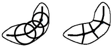
Figure 1:A bone shape (A) and its medial axis (B). (C) shows the medial axis function derived as the locus of centers of discs inscribed in the image. In (D), the shape is partitioned into

Figure 2:Skeleton extracted from 3D model. Image taken from [17].

Another explicit approach for shape representation is the part-based representation, where an

object is described by a collection of primitive shapes. Marr and Nishikara [19] explore a part-based

representation of three dimensional shapes. Biederman [3] focuses on human shape recognition

based on the simple geometric components of a shape. This Recognition-By-Components approach

is further explored in Pentland [23] where it is optimized for computer vision, and Siddiqi and

Kimia [28] expand it’s ability to remain invariant to local deformations and global changes such

In contrast to explicit methods for shape representation, implicit methods have also been explored.

The Euclidean distance transform computes the minimum distance from each point inside a shape

to the boundary of the shape. Algorithms for the Euclidean distance transform are presented in

Fabbriet alin [10], and an example is shown in Figure 3. More distance based transforms are

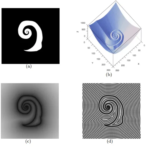
explored in [33], as shown in Figure 4. This concept is applied in the development of Voronoi

diagrams in [11], [21] and [20], shown in Figure 5.

Figure 3:A spiraled shape (a), its distance transform, where the smallest distance from each point to the border is represented by the height of a surface (b) and alternately with brightness

Figure 5:Voronoi diagram and pruned skeleton representation of image. The pruned skeleton is determined by removing relatively unimportant sections from the full Voronoi diagram

to obtain a more basic shape representation. Image taken from [20].

Also citing [5], [25] presents Deformable Shape Loci (DSL) as a representation and segmentation

method for 2D and 3D medical images. This is extended in [24], where M-reps are presented as a

means for modeling 3D solids based on the medial axis transform, shown in Figure 6. M-reps

are applied to medical images of kidneys, hippocampi and corpus collosa in [26], [12] and [29],

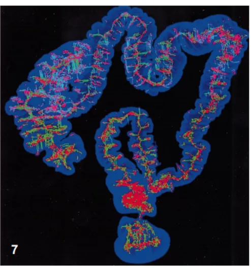
respectively. Figure 7 shows an example of M-reps applied to an image of a kidney.

Figure 6:2D illustration of (left) the traditional view of the medial locus, bitangent to the object boundary. The equivalent as an M-rep (right): a curve of hubs at the sphere center and

Figure 7:Surface rendering using M-reps. Image taken from [26].

In [14], a new implicit method for extracting properties from a shape is presented. A function is

defined on the shape; the value of the function at a particular point is the expected time that a

symmetric random walk takes to hit the boundary, given it started at that point. The authors of

[14] show that the function is actually the solution to a nonhomogeneous Poisson equation on

the shape, with homogeneous Dirichlet boundary conditions. Examples of the solution to the

Poisson equation on shapes are shown in Figures 8 and 9. Figure 8 illustrates the advantage of this

representation: it is smooth and thus differentiable on the shape interior, whereas the Eucludean

distance transform is not.

Figure 8:Left: level sets of the solution to the Poisson equation for the shape of an elephant. Right: the level sets of the distance transform for the same shape. Image taken from [14].

The random walk approach of [14] is extended in [15], where a graph based image segmentation

algorithm is presented. Similar to the method presented in the following chapters, it utilizes

Laplace’s equation. In addition, [2] uses this method to extract space-time features of human

motion, and [13] extends it by implementing Robin boundary conditions. In [32], the random walk

approach is applied to gait recognition. Each frame of a video of a person’s walk are taken and

properties of the images are extracted. Similarly, [4] applies random walks to extract properties of

shapes created as a person runs, walks or does jumping jacks, shown in Figure 10. The random

walk method introduced in [14] is applied to 3D face recognition in [18]. While these methods

focus on functions inside shapes, functions on surfaces can be used shape recognition, specifically

3D face recognition as shown in [7] and [9].

Figure 10:The solution to the Poisson equation on jumping jack, walking and running space time shapes. Image taken from [4].

The shape representation given in [14] utilized the Poisson equation in computing the mean hitting

time for any point inside a shape. A question that follows naturally is whether or not the same

computation can be done on the outside of the shape. In the following chapters, we utilize the

idea of a hitting time, as introduced in [14], which was focused on deriving and analyzing the

Poisson function and its properties on the inside of a shape. We extend this idea to develop a

III.

B

rownian

M

otion

H

itting

T

imes

We first consider the case where a particle originates at a point in the interior of the shape and

undergoes Brownian motion. The hitting time of the particle is defined as the first time the particle

hits the boundary of the shape. We are interested in the distribution of hitting time given that the

Brownian motion originates at a specific positionxinside the shape.

Now, consider a shape that has been sampled on a uniformly spaced grid. The method

de-veloped by Gorelick et al [14] utilizes the notion of random walks to extract properties of a

silhouette. These properties are defined by the expected duration of the random walks originating

at points in the shape interior.

In this chapter, we extend the analysis of [14] to show how the survival function of the Brownian

motion hitting time is the solution to a boundary value problem on the shape. In Section III.2, the

moments of the hitting time are computed from the survival function. Examples are shown in

Section III.3.

To formalize the concept of shape, we define a shape as a compact set ¯Ω ⊂ Rn_{, and we}

de-note the interior and boundary of the shape byΩand∂Ω, respectively. To formalize the concept of

hitting time, let{X(t)∈Rn_{,t≥0}denote the position of a particle undergoing Brownian motion,}

and letTBbe defined as follows:

TB=

  

inft≥0t|X(t)∈Rn\Ω¯ , X(0)∈Ω, inft≥0t|X(t)∈Ω¯ , X(0)∈Rn\Ω¯.

Therefore,TBcan be thought of as ahitting time; namely,TBis the first time that the particle hits

the boundary of the shape. We begin by considering only the particles that start inside the shape

(i.e.,X(0)∈_Ω¯_{), in which caseTBis the first exit time of the particle from ¯Ω.}

III.1

Survival Function Initial Boundary Value Problem

For any pointx∈Rn_{, we define thesurvival function S(x,t)to be the probability that the hitting}

time exceedstgiven that the particle is initially located atx; that is,

As shown in Appendix A.1.1, for pointsx∈_Ω¯_{, the survival function inndimensions satisfies the} initial boundary value problem (IBVP):

∂

∂tS(x,t)− 1

2n∆S(x,t) =0, ∀x∈Ω, t≥0,

S(x,t) =0, ∀x∈∂Ω, t≥0,

S(x, 0) =1, ∀x∈Ω. (III.2)

Now, we define the operatorLby:

L{S(x,t)}= ∂

∂tS(x,t)− 1

2n∆S(x,t). (III.3)

(III.2) can then be rewritten as:

L{S(x,t)}=0, ∀x∈Ω, t≥0,

S(x,t) =0, ∀x∈∂Ω, t≥0,

S(x, 0) =1, ∀x∈Ω. (III.4)

III.2

Moments

Thekthmoment about zero of the hitting timeTBof the Brownian motion starting at pointxinside

the shape can be computed from the survival function by:

Uk(x) =k

Z ∞

0 t

k−1_{S(x,t)dt. (III.5)}

We show in Appendix A.1.2 that multiplying each side of (III.2) by ktk−1, integrating, and

employing (III.5) yields the recursive set of boundary value problems:

− 1

2n∆Uk(x) =kUk−1(x), ∀x∈Ω,

U0(x) =1, ∀x∈Ω,

Uk(x) =0, ∀x∈∂Ω, (III.6)

for k= 1,2,....

Note that whenk=0 , the zeroth moment ofU0(x) =1, asE[TB0] =1.

Central moments, denotedVk(x)can then be computed as:

Vk(x) =

k

∑

m=0

k m

Standardized momentsWk(x)can then be computed from the central moments as follows:

Wk(x) =

Vk(x)

V2k/2

. (III.8)

For example, the standard deviation, skewness, and kurtosis are given by:

W2(x) =

q

V2(x), (III.9)

W3(x) = V3

(x)

V2(x)3/2

, (III.10)

W4(x) = V4

(x)

V2(x)2

, (III.11)

respectively.

III.3

Computational Examples of Moments

In this section, we illustrate the hitting time and higher moments defined in Section III.2 for a

shape that represents a silhouette of a horse.

The mean hitting time U1(x), is shown in Figure 11. The standardized moments of the hit-ting time, computed from the central moments as in (III.9) through (III.11) and denotedWk(x)are

shown (along with variance) in Figure 12. The moments about zeroUk(x), and central moments

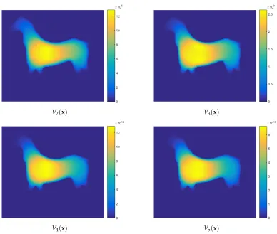
Vk(x)are shown in Figures 13 and 14, respectively.

The level sets ofUk(x),Vk(x)andWk(x)are smoothed versions of the bounding contour. The head,

legs and tail exhibit much smaller values than those inside the torso for the moments about zero,

Uk(x), the central moments,Vk(x), and the standard deviationW2(x). The skewness,W3(x)and kurtosis,W4(x)achieve maximum values on the ears, tail and legs while the values in the torso are relatively small. Notice that the skewness and kurtosis values are noisy on the boundaries of the

shape and there are points with values much larger than the surrounding values, so it is difficult

to visualize the results. We found that using the reciprocals of the skewness and kurtosis provides

a better visualization. The reciprocal of the skewness and kurtosis, _W1

3(x) and

1

W4(x), respectively,

achieve maximum values both near the centroid, similar toUk(x)andVk(x), but also on the feet

Silhouette Mean

U1(x)

Variance

V2(x)

Standard Deviation

W2(x)

Skewness

W3(x)

Reciprocal of Skewness

1 W3(x)

Kurtosis

W4(x)

Reciprocal of Kurtosis

1 W4(x)

U1(x) U2(x)

U3(x) U4(x)

V2(x) V3(x)

V4(x) V5(x)

Figure 14:kthCentral Moments ofTBwhereX(0)∈Ω¯.

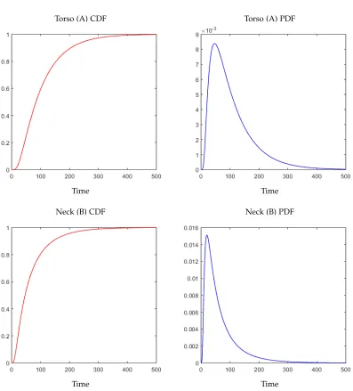
In Figures 15 and 16, the probability density function and cumulative distribution function ofTB

are computed for various points on the head, neck, leg and centroid of a horse silhouette.

Notice thatTBtakes on smaller values when the random walk begins at a point in an extremity of

the horse such as at point C or D, shown in Figures 16, compared to those that begin at points in

Torso (A) CDF

Time

Torso (A) PDF

Time

Neck (B) CDF

Time

Neck (B) PDF

Time

(a)Head (C) CDF

Number of Steps in Random Walk

(b)Head (C) PDF

Number of Steps in Random Walk

(c)Leg (D) CDF

Number of Steps in Random Walk

(d)Leg (D) PDF

Number of Steps in Random Walk

IV.

B

rownian

M

otion

A

ugmented with

N

atural

L

ifetime

In Chapter III, we considered representations that are defined only on a closed shape. In this

chapter, we expand these representations to be defined everywhere inRn, including the shape

exterior.

Random walks in two dimensions are null recurrent, meaning the probability that the

ran-dom walk will return to its starting position is equal to one, however, the expected value of the

number of steps it takes to return to that position is infinite. This implies that the mean hitting

time is infinite, and is not useful in providing a representation whose values outside the shape can

be used to discriminate between different shapes. (Note that random walks in three dimensions or

higher are transient).

As an alternative to using the mean hitting time alone, we assign to the particle an exponentially

distributed lifetimeTL, that is independent ofX(t), guaranteeing that the Brownian motion will

eventually terminate. Incorporating this dying time, or natural lifetime, allows us to measure the

minimum of the times required to(1)hit the boundary of the shape, as in the previous section, or

(2)reach the end of its natural lifetime, and this new quantity will have a finite expected value. In this section, we derive an initial boundary value problem describing the survival function for

the minimum ofTBandTL. We then illustrate some properties.

IV.1

Survival Function Initial Boundary Value Problem

As in Section III.1, we define a shape as a compact set ¯Ω⊂Rn_{, and denote the interior byΩand}

boundary by∂Ω. Again we consider a particle undergoing Brownian motion, and denote the

position of the particle{X(t),t≥0}. Recall the hitting time of the particle,TB, defined as the first

time at which the particle crosses the boundary of the shape, i.e.

TB=

  

inft≥0t|X(t)∈Rn\Ω¯ , X(0)∈Ω, inft≥0t|X(t)∈Ω¯ , X(0)∈Rn\Ω¯.

defineTL to be the natural lifetime of the particle. We will assume thatTLis independent ofX(t)

andTBand thatTLhas an exponential distribution with parameterλ, so that P(T>t) =e−λtfor

t≥0 and 1 otherwise.

Now, we define T = min(TB,TL), and we define Sβ(x,t) to be the probability that the

mini-mum of the hitting time and the lifetime exceedst, given that the particle is initially located atx, andβ= _λ1 =E[TL]. That is:

S_β(x,t) =PT>t|X(0) =x,TL∼exp

1

β

. (IV.1)

As shown in Appendix A.2.1, for pointsx∈Rn_{\Ω¯, the survival functionS}

β(x,t)can be written

as the following initial boundary value problem:

∂

∂tSβ(x,t)− 1

2n∆Sβ(x,t) +

1

βSβ(x,t) =0, ∀x∈R

n_{\∂Ω, t≥0,}

Sβ(x,t) =0, ∀x∈∂Ω, t≥0,

Sβ(x, 0) =1, ∀x∈Ω. (IV.2)

Applying the definition ofLfrom (III.3) allows us to write (IV.2) as:

L+ 1

βI

S_β(x,t) =0, ∀x∈Rn_\

∂Ω¯, t≥0,

S_β(x,t) =0, ∀x∈∂Ω, t≥0,

Sβ(x, 0) =1, ∀x∈Ω. (IV.3)

In the following sections, we examine various properties ofTgivenX(0).

IV.2

Moments

Thekth_{moment ofTgivenX(0) =xis denoted byU}

k(x), and can be computed from the survival

function by:

Uk,β(x) =k

Z ∞

0 t

k−1_S

β(x,t)dt. (IV.4)

As shown in Appendix A.2.2, by multiplying both sides of the inital boundary value problem

value problem:

−kUk−1,β(x)−

1

2n∆Uk,β(x) +

1

βUk,β(x) =0, ∀x∈R

n_\∂Ω,

Uk,β(x) =0, ∀x∈∂Ω,

U0,β(x) =1, ∀x∈R

n_{. (IV.5)}

or:

−kUk−1,β(x) +

1 βI−

1 2n∆

Uk,β(x) =0, ∀x∈R

n_\∂Ω,

U1,β(x) =β, ∀x∈∂Ω, (IV.6)

whereβis the expected value of exponentially distributed random variableTLthe natural lifetime

of the particle.

Notice that whenk=1, (IV.5) can be rewritten as the following Helmholtz equation: ∆U1,β(x)−

2n

β U1,β(x) =−2n, ∀x∈R

n_\∂Ω,

U1,β(x) =β, ∀x∈∂Ω. (IV.7)

Central moments, denotedVk(x), can then be computed as:

Vk,β(x) =

k

∑

m=0

k m

(−1)k−mUm,β(x)U1,β(x)

k−m_{, k=1, 2, ... (IV.8)}

Standardized momentsWk,β(x)can then be computed from the central moments as follows:

Wk,β(x) =

Vk,β(x)

V2,β(x) k

2

, k=1, 2, ... (IV.9)

IV.3

Discretization of IBVP

Recall (IV.2), the initial boundary value problem:

∂

∂tSβ(x,t)− 1

2n∆Sβ(x,t) +

1

βSβ(x,t) =0, ∀x∈R

n_{\∂Ω, t≥0,}

S_β(x,t) =0, ∀x∈∂Ω, t≥0,

Sβ(x, 0) =1, ∀x∈Ω¯.

IV.3.1 Spatial Discretization

Suppose ¯Γ⊂Ω¯ is an-dimensional uniform grid of points. Each grid pointxhas neighborhood

N(x) =Γ¯∩

x±hej|j=1, . . . ,n , whereejis thejthcolumn of then-dimensional identity matrix,

andhis the grid spacing. The interiorΓcontains all points in ¯Γthat have 2nneighbors (i.e., points

for which|N(x)|=2n), and the discrete boundary∂Γ=Γ¯\Γ.

We can rewrite the spatial Laplacian of the survival function as the sum of its second partial

derivatives in space. For points inRn\∂Γ¯ we have:

∆Sβ(x,t) =

n

∑

i=1 ∂2

∂x2_iSβ

(x,t). (IV.10)

Implementing the centered difference approximation for the second derivative gives:

∆Sβ(x,t)≈

n

∑

i=1

S_β(x−hei,t)−2Sβ(x,t) +Sβ(x+hei,t)

h2 ,

whereeiis theith unit vector. That is,

ei=

            0 .. . 1 .. . 0             ,

where 1 is in theith position of the 1×nvectorei.

Bringing the term−2S_β(x,t)outside the summation yields: ∆S_β(x,t)≈ −2n

h2Sβ(x,t) +

n

∑

i=1

S_β(x−hei,t) +Sβ(x+hei,t)

h2 . (IV.11)

Substituting (IV.11) into (IV.2) gives the discrete spatial approximation:

∂

∂tSβ(x,t)− 1 2n

"

−2n

h2Sβ(x,t) +

n

∑

i=1

S_β(x−hei,t) +Sβ(x+hei,t)

h2

#

+ 1

βSβ(x,t) =0. (IV.12) Simplifying gives the following:

∂

∂tSβ(x,t) +

1

h2+

1 β

Sβ(x,t)−

1 2n

n

∑

i=1

S_β(x−hei,t) +Sβ(x+hei,t)

IV.3.2 Time Discretization

Discretizing (IV.13) forward in time with time step∆τyields:

S_βx,tk+1_−S

β

x,tk

τ =−

1

h2 +

1 β

Sβ

x,tk+ 1

2nh2

n

∑

i=1

h

Sβ

x−hei,tk

+Sβ

x+hei,tk

i

.

(IV.14)

Multiplying both sides of (IV.14) byτand addingS_β

x,tkto both sides gives:

Sβ

x,tk+1=Sβ

x,tk−τ

1

h2+

1 β

Sβ

x,tk+ τ

2nh2

n

∑

i=1

h

Sβ

x−hei,tk

+Sβ

x+hei,tk

i

.

(IV.15)

Combining like terms yields the explicit iteration:

S_βx,tk+1=

1−τ

β− τ

h2

S_βx,tk+ τ

2nh2

n

∑

i=1

h

S_βx−hei,tk

+S_βx+hei,tk

i

. (IV.16)

Alternatively, discretizing backward in time with step sizeτyields:

S_βx,tk+1_−S

β

x,tk

τ =−

1

h2+

1 β

Sβ

x,tk+1

+ 1

2nh2

n

∑

i=1

h

S_βx−hei,tk+1

+S_βx+hei,tk+1

i

. (IV.17)

Multiplying by−τand addingS_β

x,tk+1to both sides yields:

Sβ

x,tk=Sβ

x,tk+1+ τ

h2Sβ

x,tk+1+τ

βSβ

x,tk+1

− τ

2nh2

n

∑

i=1

S_β(x−hei,t) +Sβ(x+hei,t)

. (IV.18)

Finally, combining like terms gives:

Sβ

x,tk= (1+ τ

h2+

τ

β)Sβ

x,tk+1− τ

2nh2

n

∑

i=1

h

Sβ

x−ei,tk+1

+Sβ

x+ei,tk+1

i

. (IV.19)

While the explicit time step yields a faster iteration, the time step must be very small to avoid

instability. The implicit iteration requires solving a system of equations at each iteration but is

IV.4

Discretization of Moment BVPs

Recall (IV.5):

−kUk−1,β(x)−

1

2n∆Uk,β(x) +

1

βUk,β(x) =0 ∀x∈ I,

U1,β(x) =β ∀x∈∂I. (IV.20)

where Uk,β(x) is thekth moment of the survival function of a particle whose natural lifetime

follows the exponential distribution with expected valueβ. Iis the image that contains the shape ¯Ω

Also recall the definition of the Laplace operator:

∆Uk,β(x) =

n

∑

i=1 ∂2

∂x2_iUk,β(x). (IV.21)

Implementing the centered difference approximation of the second derivative in (IV.21) gives:

∆Uk,β(x) =

1 h2

n

∑

i=1

h

Uk,β(x−hei)−2Uk,β(x) +Uk,β(x+hei)

i

,

=−2n

h2Uk,β(x) +

1 h2

n

∑

i=1

h

Uk,β(x−hei) +Uk,β(x+hei)

i

. (IV.22)

Substituting into (IV.5) gives:

−kUk−1,β(x)−

1 2n

"

−2n

h2Uk,β(x) +

1 h2

n

∑

i=1

h

Uk,β(x−hei) +Uk,β(x+hei)

i #

+ 1

βUk,β(x) =0, (IV.23)

or,

−kUk−1,β(x) +

1

h2Uk,β(x)−

1 2nh2

n

∑

i=1

h

Uk,β(x−hei) +Uk,β(x+hei)

i

+ 1

βUk,β(x) =0. (IV.24) Combining like terms yields:

−kUk−1,β(x) +

1

h2+

1 β

Uk,β(x)−

1 2nh2

n

∑

i=1

h

Uk,β(x−hei) +Uk,β(x+hei)

i

=0. (IV.25)

It follows that we can find the discretization of the mean, variance and higher order moments by

substituting values ofk=1, 2, 3, .. . Substitutingk=1 into (IV.25) yields the discretization of the first moment, or mean,U1,β(x):

−U0,β(x) +

1

h2+

1 β

U1,β(x)−

1 2nh2

n

∑

U1,β(x−hei) +U1,β(x+hei)

U0,β(x)is the zeroth moment of the survival function, which is equal to 1. So we have:

−1+

1

h2 +

1 β

U1,β(x)−

1 2nh2

n

∑

i=1

U1,β(x−hei) +U1,β(x+hei)

=0, or,

1

h2+

1 β

U1,β(x)−

1 2nh2

n

∑

i=1

U1,β(x−hei) +U1,β(x+hei)

=1. (IV.26)

With the addition of the boundary conditions, (IV.26) becomes:

1

h2+

1 β

U1,β(x)−

1 2nh2

n

∑

i=1

U1,β(x−ei) +U1,β(x+ei)

=1 ∀x∈Rn_\∂Ω,

U1,β(x) =β ∀x∈∂Ω. (IV.27)

Substitutingk=2 into (IV.25) yields the discretization of the second moment ofT.

−U1,β(x) +

1

h2 +

1 β

U2,β(x)−

1 2nh2

n

∑

i=1

U2,β(x−hei) +U2,β(x+hei)

=0, (IV.28)

or,

1

h2 +

1 β

U2,β(x)−

1 2nh2

n

∑

i=1

U2,β(x−hei) +U2,β(x+hei)

=U1,β(x). (IV.29)

In the following sections we explore the results obtained by solving (IV.5) on a collection of shapes.

We show analytical solutions on spheres and numerical solutions on other more complicated

shapes.

IV.5

Analytical Examples

In this section we show a special case of the mean hitting time and the analytical solution on a

circle or sphere ofn-dimensions.

As shown in Appendix A.2.3, the first moment of the mean survival function ofTgiven that∂Ωis

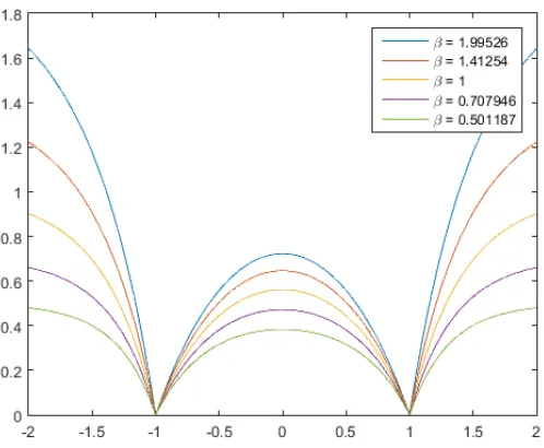
a circle of radiusRisU1,β(r) =Y1,β(kxk), where:

Y1,β(r) =β−

β I0 2R √ β I0 2r p β !

r<R, (IV.30)

Y1,β(r) =β−

β K0 2R √ β K0 2r p β !

Figure 17:Y1,βfor varying values ofβon a circle of radiusR=1.

I0is a modified Bessel function of the first kind andK0is a modified Bessel function of the second

kind. Plots of (IV.30) and (IV.31) are shown in Figure 17 for several values ofβ.

IV.6

Computational Examples of Mean Hitting Time

In this section,U1(x)andU1,β(x)are computed for various shapes. Figures 18, 20 and 22 show

the shape silhouettes, mean hitting times as in Section III.3, mean dying times as in Section IV.2

and the logarithms of mean dying times.

Figures 19, 21 and 23 show the log mean dying time, log

U1,β(x)

, for various values ofβon a

horse silhouette, a circle and a triangle with noisy boundaries, respectively. Asβincreases, the

(a)Horse Silhouette (b)Mean Hitting TimeU1(x)

(c)U1,β(x)whereβ=100 (d)log[U1,β(x)]whereβ=100

Figure 18:Mean hitting timeU1(x)and mean dying time,U1,β(x), for pointsxboth inside and

(a)β=5 (b)β=10

(c)β=50 (d)β=100

(e)β=500 (f)β=1000

(g)β=5000 (h)β=10000

Figure 19:Log mean dying time, log

U1,β(x)

(a)Circle Silhouette (b)Mean Hitting Time

(c)U1,β(x)whereβ=100 (d)log[U1,β(x)]whereβ=100

Figure 20:Mean dying time,U1,β(x), for pointsxboth inside and outside the boundary of the

(a)β=5 (b)β=10

(c)β=50 (d)β=100

(e)β=500 (f)β=1, 000

(g)β=5, 000 (h)β=10, 000

Figure 21:Log mean dying time, log

U1,β(x)

(a)Noisy Triangle Silhouette (b)Mean Hitting Time

(c)U1,β(x)whereβ=100 (d)log[U1,β(x)]whereβ=100

Figure 22:Mean dying time,U1,β(x), for pointsxboth inside and outside the boundary of the

(a)β=5 (b)β=10

(c)β=50 (d)β=100

(e)β=500 (f)β=1, 000

(g)β=5, 000 (h)β=10, 000

Figure 23:Log mean dying time, log

U1,β(x)

IV.7

Computational Examples of Moments

In this section, we compute the dying time and higher moments defined in Section IV.2 for various

silhouette images.

The standardized moments of the dying time,Wk,β(x), are shown in Figures 24, 27 and 30 for a

horse, circle and triangle silhouette, respectively. Figures 25, 28 and 31 show the moments about

zeroUk,β(x). The central momentsVk,β(x)are shown in Figures 26, 29, and 32 .

Similar to the hitting time moments in Section III.3, the level sets ofUk,β(x),Vk,β(x)andWk,β(x)are

smoothed versions of the bounding contour. Inside the shape, the maximum values are achieved

near the centroid, and outside the shape the maximum values are near the image boundary

for the moments about zero,Uk,β(x), the central moments,Vk,β(x), and the standard deviation

W2,β(x). The skewness,W3,β(x), and kurtosisW4,β(x)achieve maximum values near the shape

boundary.

As in Section III.3, the skewness and kurtosis values are noisy on the boundaries of the shape

and using the reciprocals of the skewness and kurtosis, _W1

3,β(x) and

1

W4,β(x), provides a better

Variance

V2,100(x)

Standard Deviation

W2,100(x)

Skewness

W3,100(x)

Reciprocal of Skewness

1 W3,100(x)

Kurtosis

W4,100(x)

Reciprocal of Kurtosis

1 W4,100(x)

U1,100(x) U2,100(x)

U3,100(x) U4,100(x)

V2,100(x) V3,100(x)

V4,100(x) V5,100(x)

Variance

V2,100(x)

Standard Deviation

W2,100(x)

Skewness

W3,100(x)

Reciprocal of Skewness

1 W3,100(x)

Kurtosis

W4,100(x)

Reciprocal of Kurtosis

1 W4,100(x)

U1,100(x) U2,100(x)

U3,100(x) U4,100(x)

V2,100(x) V3,100(x)

V4,100(x) V5,100(x)

Variance

V2,100(x)

Standard Deviation

W2,100(x)

Skewness

W3,100(x)

Reciprocal of Skewness

1 W3,100(x)

Kurtosis

W4,100(x)

Reciprocal of Kurtosis

1 W4,100(x)

U1,100(x) U2,100(x)

U3,100(x) U4,100(x)

V2,100(x) V3,100(x)

V4,100(x) V5,100(x)

V.

C

lassification

E

xperiments

In order to determine the efficacy of utilizing the features presented in Section IV.7, we perform

classification experiments using two datasets. The data, experiments, and results are described in

the following sections.

V.1

Data

We present results using two publicly available datasets.

The first is a collection of natural silhouettes. There are 12 classes of images (cups, hands, humans,

horses, birds, fish, rays, cats, dogs and elephants), with 490 images total, and Figure 33 shows

examples from each class of silhouettes. This particular collection of silhouettes was first used in

[14].

The second dataset is the MNIST database of handwritten digits [16], with a training set of 60,000

examples and a test set of 10,000 examples.

V.2

Experimental Setup

To determine the efficacy of utilizing the dying time moments presented in Section IV.2 in shape

classification, we use support vector machines, or SVMs, to classify images based on the proposed

features. The classification is performed using a multiclass SVM with a one-versus-all method, as

implemented in MATLAB, with 20% of the images used as training data for the natural silhouettes

dataset, and 86% used to train the classifier for the MNIST handwritten digit database.

The shape descriptors used were mean, standard deviation, skewness, and kurtosis, as described

in Sections III.2 and IV.2. These were computed for each image using both the hitting time and

the dying time. When using the hitting time shape descriptor, the values were computed inside

the shape. When using the dying time, the values were computed both inside and outside the

shape.

V.3

Results

We quantified the results using confusion matrices, which indicate the number of true positives

Figure 34:Sample images from MNIST database.

performance measures derived from each confusion matrix are as follows:

accuracy (A):

A= TP+TN

TP+TN+FP+FN, (V.1)

precision (P):

P= TP

TP+FP, (V.2)

sensitivity (Se):

Se= TP

TP+FN, (V.3)

and specificity (Sp):

Sp= TN

FP+TN. (V.4)

We performed the classification four different ways. First, we used the hitting time from Chapter

III inside the shape. Second, we used the dying time from Chapter IV both inside and outside

the shape. Third, with dying time just outside the shape. Finally, we performed the classification

with the hitting time moments inside the shape and dying time moments outside the shape fused

together.

Tables 1 and 2 show the natural silhouette and handwritten digit classification experiment results,

respectively. The average accuracy (AA), average precision (AP), average sensitivity (ASe) and

inside the shape (HT), dying time inside and outside the shape (DT), dying time outside the shape

only (DTOut) and the hitting time inside the shape fused with the dying time outside the shape

(Fused). The remaining rows show the average accuracy for each method across all classes.

Table 1, shows the results of classification based the dying time outside the shape fused with the

hitting time inside the shape outperformed the other features in accuracy, precision, sensitivity and

specificity over all twelve classes of natural silhouettes. Specifically, classes 1 (mug), 4 (horse), 6

(shark), 7 (fish), 8 (stingray), 9 (cat), 10 (dog) and 12 (elephant) showed an improvement in accuracy.

As we saw with the the natural silhouettes, when classifying the handwritten digits based on the

dying time outside the shape fused with the hitting time inside the shape outperformed the other

features in accuracy, precision, sensitivity and specificity over all 10 classes of digits, as shown in

No. of Samp HT DT DTOut Fused

Average Accuracy - 94.14 92.03 91.99 95.39

Average Precision - 64.46 48.89 49.73 74.22

Average Sensitivity - 67.39 49.46 48.76 72.26

Average Specificity - 96.82 95.64 95.62 97.47

Class 1: Mug 26 98.71 95.09 96.64 99.22

Class 2: Hand 26 99.74 96.90 95.87 99.48

Class 3: Person 55 97.67 97.67 97.93 97.67

Class 4: Horse 80 83.46 91.21 91.47 91.73

Class 5: Bird 50 89.92 84.75 83.98 89.41

Class 6: Shark 43 96.64 94.83 94.57 96.90

Class 7: Fish 28 95.87 91.47 91.47 97.93

Class 8: Stingray 47 93.54 86.56 87.60 94.32

Class 9: Cat 42 89.66 86.30 85.79 92.51

Class 10: Dog 49 91.73 88.11 88.63 91.99

Class 11: Hawk 17 96.64 96.38 97.16 96.90

Class 12: Elephant 27 96.12 95.09 92.76 96.64

No. of Samp HT DT DTOut Fused

Average Accuracy - 88.46 88.26 87.94 90.99

Average Precision - 41.29 40.44 38.97 54.21

Average Sensitivity - 39.29 37.57 36.53 52.37

Average Specificity - 93.66 93.56 93.37 95.07

Class 0 10,000 86.99 85.84 85.75 93.51

Class 1 10,000 97.34 96.18 95.77 98.08

Class 2 10,000 87.36 85.94 86.56 88.26

Class 3 10,000 86.22 87.47 87.18 88.82

Class 4 10,000 86.78 87.82 86.59 89.34

Class 5 10,000 88.21 88.66 88.24 89.58

Class 6 10,000 87.57 91.60 90.64 91.18

Class 7 10,000 90.93 87.88 87.80 92.02

Class 8 10,000 85.85 85.50 84.00 88.87

Class 9 10,000 87.33 85.67 86.89 90.28

Table 2: Digits classification results. Class rows show per-class accuracy. All quantities are percentages, with the exception of the number of samples.

The following figures provide a visual representation of the comparison of the confusion matrices

that report the classification results using the hitting time moments and the hitting time moments

inside the shape fused with the dying time moments outside the shape.

Figures 35 and 36 show the true positives, or horses correctly classified as horses, from the

hitting time and fused hitting time and dying time experiments, respectively. The hitting time

experiment resulted in 55 true positives and the hitting time fused with dying time resulted in 52

true positives.

Figures 37 and 38 show the false positives, or non-horse images incorrectly classified as horses,

from the hitting time and fused hitting time and dying time experiments, respectively. Here we

see that fusing the hitting time and dying time features decreases the number of false positives by

63.6%, with 55 false positives using only the hitting time and 20 false positives with the hitting

time and dying time fused.

Figures 39 and 40 show the false negatives, or horse images incorrectly classified as non-horses,

9 false negatives using the hitting time features, and 12 when using the hitting time fused with

dying time.

The true negatives, all other images correctly classified as non-horses, are not shown. There were

371 hitting time true negatives and 403 fused hitting time and dying time true negatives.

Figure 37: Class 4 (horse) false positives from hitting time experiment.

Figure 39: Class 4 (horse) false negatives from hitting time experiment.

VI.

C

onclusion

Solutions to the Helmholtz equation provide meaningful information about a shape silhouette

that was shown to be useful in classification. Using these features, we were able to improve an

existing method of shape representation. The features extracted with this representation allowed

for an improvement in the effectiveness of shape classification.

First, in Chapter III we established the survival function and its corresponding initial value

problem, and showed its mean and higher order moments. We then illustrated these features

computed inside various shape silhouettes.

In Chapter IV, we extended the analysis to the outside of the shape by incorporating a natural

lifetime into the survival function. As before, we illustrated these features computed for silhouette

images, both inside and outside the silhouette boundary.

Finally, in Chapter V we used the features developed in the preceding chapters to perform

classification experiments to determine the efficacy of the new features. We performed the

experiment on two databases of images, both natural shape silhouettes and handwritten numerals,

and saw an increase in accuracy and decrease in the rate of false positives when using the new

features computed from the survival function outside the shape in conjunction with the survival

function inside the shape.

A possibility for future research is to extend this approach to higher dimensions, as we have

explored only the representation and classification of shapes in two dimensions. Additionally,

the Helmholtz shape classification approach could be extended to space-time action recognition,

VII.

A

cknowledgments

First and foremost, I must express my sincere gratitude to my advisor Dr. Nathan Cahill, for his

enthusiasm, patience and immense knowledge. His drive and dedication motivated me throughout

my work. Dr. Cahill is a true mentor and his contributions were invaluable to this thesis. I am

also indebted to my committee members for providing their insight and expertise. Additionally,

I’d like to thank the rest of the faculty in the RIT Department of Mathematics, as well as my

classmates for their continued help and inspiration.

I must also thank my friends and family for the never ending love and support they have provided.

A special thanks to Adam for his understanding and for cooking me countless dinners while

I worked, and to the rest of the Candela family for their continuous encouragement. Finally,

thanks to Abby and my parents for always being in my corner and supporting my goals and

A.

A

ppendix

A.1

Brownian Motion Inside a Shape

A.1.1 Hitting Time Boundary Value Problem

This appendix establishes that the survival functionS(x,t)defined in (III.1) satisfies the IBVP given in (III.2).

Suppose ¯Γ⊂_Ω¯ _{is an-dimensional uniform grid of points. Each grid pointxhas neighborhood}

N(x) =Γ¯∩

x±hej|j=1, . . . ,n , whereejis thejthcolumn of then-dimensional identity matrix,

andhis the grid spacing. The interiorΓcontains all points in ¯Γthat have 2nneighbors (i.e., points

for which|N(x)|=2n), and the discrete boundary∂Γ=Γ¯\Γ.

Consider a particle that undergoes a symmetric random walk on ¯Γ. Let τ be the finite time

between steps of the random walk. The position of the particle is given byX(t), wheretrepresents continuous time; hence,X(t)is piecewise constant with steps att=kτ,k=0, 1, 2, . . .. The hitting timeTBcorresponds to the first time the particle lands in∂Γ; i.e. TB=inft≥0{t|X(t)∈∂Γ}. The survival function S(x,t) is defined as in (III.1); i.e., S(x,t) = P(TB>t|X(0) =x). If we

condition on the first step of the random walk, for points inΓwe have:

S(x,t+τ) =Pr{TB>t+τ|X(0) =x}

=

n

∑

j=1

 

Pr

TB>t+τ|X(0) =x,X(1) =x+hej PrX(1) =x+hej|X(0) =x

+ Pr

TB>t+τ|X(0) =x,X(1) =x−hej PrX(1) =x−hej|X(0) =x

  = 1 2n n

∑

j=1

 

Pr

TB>t|X(0) =x+hej

+ Pr

TB>t|X(0) =x−hej

  = 1 2n n

∑

j=1

S x+hej,t+S x−hej,t. (A.1)

Alternatively, expandingS(x,t)abouttyields:

S(x,t+τ) =S(x,t) +τ∂

∂tS(x,t) +O

τ2

, (A.2)

and so combining (A.1) and (A.2) gives:

S(x,t) +τ∂

∂tS(x,t) = 1 2n

n

∑

j=1

S x+hej,t+S x−hej,t+O

τ2

ExpandingS(x,t)aboutxyields:

S x±hej,t

=S(x,t)±hSxj(x,t) +

h2 2

∂2

∂x2_jS

(x,t) +Oh3, (A.4)

so

S x+hej,t+S x−hej,t=2S(x,t) +h2

∂2

∂x2_jS(x,t) +O

h3, (A.5)

and (A.3) can be written as:

S(x,t) +τ∂

∂tS(x,t) =S(x,t) +

h2 2n

n

∑

j=1

"

∂2

∂x2_jS(x,t)

#

+Oτ2

+Oh3. (A.6)

Rearranging terms and dividing both sides of (A.6) byτyields:

∂

∂tS(x,t)− 1 2n h2 τ n

∑

j=1

"

∂2

∂x2_jS(x,t)

#

=O(τ) +O

h3 τ

. (A.7)

Taking the limit of both sides of (A.7) ashandτapproach zero while h_τ2 is fixed at 1 yields: ∂

∂tS(x,t)− 1

2n∆S(x,t) =0, (A.8)

where∆is the spatial Laplacian. (A.8) now applies for allx∈Ωandt≥0. Note thatTB=0 on

the boundary, soS(x,t) =0 forx ∈∂Ω. Furthermore, S(x, 0) = 1 for any point on the interior, and hence,S(x,t)satisfies (III.2).

A.1.2 Hitting Time Moments

This appendix establishes the moments of the hitting time inside a shape.

Recall (A.8):

∂

∂tS(x,t)− 1

2n∆S(x,t) =0, ∀x∈Ω, t≥0,

S(x,t) =0, ∀x∈∂Ω, t≥0,

S(x, 0) =1, ∀x∈Ω. (A.9)

Multiplying both sides byktk−1yields:

ktk−1∂

∂tS(x,t)− 1 2nkt

We integrate (A.10) with respect totas follows:

Z ∞

0 kt

k−1∂

∂tS(x,t)dt−

Z ∞

0 1 2nkt

k−1_{∆S(x,t)dt=0. (A.11)}

Constants can be brought outside the integral, as can the spatial Laplacian operator:

k

Z ∞

0 t

k−1∂

∂tS(x,t)dt− 1 2nk∆

Z ∞

0 t

k−1_{S(x,t)dt=0. (A.12)}

Recall from (III.5):

Uk(x) =k

Z ∞

0 t

k−1_{S(x,t)dt. (A.13)}

Substituting this into the second term of (A.12) yields:

k

Z ∞

0 t

k−1∂

∂tS(x,t)dt− 1

2n∆Uk(x) =0. (A.14)

The first term of (A.14) can be integrated by parts as follows:

k

Z ∞

0 t

k−1∂

∂tS(x,t)dt= kt

k−1_S(x,t)

∞

0 −k(k−1)

Z ∞

0 t

k−2_S(x,t)dt

=klim

t→∞t

k−1_{S(x,t)−0−k(k−1)}Z ∞ 0 t

k−2_S(x,t)dt

=0−0−k(k−1)

Z ∞

0 t

k−2_S(x,t)dt

=−k(k−1)

Z ∞

0 t

k−2_{S(x,t)dt. (A.15)}

Note that the limit above limt→∞tk−1S(x,t) is in an indeterminate form (0·∞). This can be rewritten as limt→∞ tk−11

S(x,t)

, and by L’Hospital’s Rule, after differentiatingk−1 times, the limit is

zero.

We can substitute (A.13) withkreplaced byk−1 into (A.15):

k

Z ∞

0 t

k−1∂

∂tS(x,t)dt=−kUk−1(x), and the integral becomes

− 1

2n∆Uk(x) =kUk−1(x), ∀x∈Ω,

U0(x) =1, ∀x∈Ω,

Uk(x) =0, ∀x∈∂Ω, (A.16)

for k= 1,2,....

A.2

Brownian Motion Augmented with Natural Lifetime

A.2.1 Survival Function Boundary Value Problem

Lemma 1. The survival function of the minimum of the hitting time and natural lifetime is equivalent to:

Sβ(x,t) =e −t

β_{S(x,t). (A.17)}

Proof. The survival function of the minimum of the hitting time and natural lifetimeTL is:

Sβ(x,t) =P(T>t|X(0) =x), (A.18)

as defined in (IV.1). We define the density function ofTL as:

fTL(s) =

d

dsP(TL<s) (A.19)

= d

ds

h

1−e−s/βi _(A.20)

= 1

βe

−s/β_{, (A.21)}

and the conditional density function ofTL givenX(0)as:

fT_L|X(0)(s) =

d

dsP(TL <s|X(0) =x). (A.22)

Conditioning onTLallows us to write (A.18) as:

Sβ(x,t) =

Z ∞

0 P

(min(TL,TB)>t|X(0) =x,TL=s)fTL|X(0)(s)ds. (A.23)

Recall that the natural lifetime of the particle and its initial position,TLandX(0)respectively, are

independent. Also, the hitting time of the particle and the natural lifetime of the particle,TBand

TL, are independent of one another. So, (A.23) becomes:

Sβ(x,t) =

Z ∞

0 P(min(s,TB)>t|X(0) =x)fTL(s)ds. (A.24) From (A.21), we have that fTL(s) =

1

βe

−s/β_{, so (A.24) becomes:}

S_β(x,t) = 1

β

Z ∞

0 P(min(s,TB)

>t|X(0) =x)e−s/β_{ds. (A.25)}

Splitting the integral ats=tgives: S_β(x,t) = 1

β

Z t

0 P

(min(s,TB)>t|X(0) =x)e−s/βds

+ 1

β

Z ∞

Notice that fors∈[0,t],P(min(s,TB)>t|X(0) =x) =0, so (A.26) simplifies to:

Sβ(x,t) =

Z ∞

t P(min(s,TB)>t|X(0) =x)e

−s/β_{ds. (A.27)}

In the intervals= [t,∞]we have:

P(min(s,TB)>t|X(0) =x) =P(TB>t|X(0) =x). (A.28)

and so:

Sβ(x,t) =

Z ∞ t P

(TB>t|X(0) =x)e−s/βds.

P(TB >t|X(0) =x)is independent ofsand can be moved outside the integral. Hence:

Sβ(x,t) =P(TB>t|X(0) =x)

Z ∞ t e

−s/β_{ds. (A.29)}

Substituting (III.1) into (A.29) gives:

Sβ(x,t) =S(x,t)

Z ∞ t e

−s/β_{ds. (A.30)}

We then evaluate the integral in (A.30) to obtain:

Sβ(x,t) =e

−t/β_{S(x,t). (A.31)}

Recall (III.2):

L[S(x,t)] =0, ∀x∈Ω, t≥0,

S(x,t) =0, ∀x∈∂Ω, t≥0,

S(x, 0) =1, ∀x∈Ω.

This boundary value problem was established in Appendix A.1.1 for the survival function of the

hitting timeTL given that a particle undergoes Brownian motion beginning at pointx⊂Ω.

Now, we will define a similar boundary value problem for the case where the random walk is

started at a point outside of the shape . First, note that:

L

S_β(x,t)

= ∂

∂tSβ(x,t)− 1

2n∆Sβ(x,t). (A.32)

Substituting (A.31) into (A.32) yields the following:

L

S_β(x,t)

= ∂

∂te

−t/β_S(x,t)− 1

2n∆e

Differentiating the first term on the right hand side of (A.33) and exploiting the linearity of the

spatial Laplacian gives:

L

S_β(x,t)

=e−t/β ∂

∂tS(x,t)− 1 βe

−t/β_S(x,t)− 1

2n∆e

−t/β_{S(x,t), (A.34)}

=e−t/β

∂

∂tS(x,t)− 1

βS(x,t)− 1

2n∆S(x,t)

. (A.35)

Recall (III.2), which states:

∂

∂tS(x,t)− 1

2n∆S(x,t) =0, ∀x∈Ω, t≥0. Substituting forSβ(x,t)into (A.35) gives:

L

S_β(x,t) =e−t/β

−1

βS(x,t)

.

This can be rewritten as a homogeneous partial differential equation:

L

Sβ(x,t) +

1 βe

−t/β_{S(x,t) =0, (A.36)}

which, in light of (A.31), can be rewritten as:

L

Sβ(x,t) +

1

βSβ(x,t) =0. (A.37)

Recall from (III.2) the boundary conditionS(x,t) =0 and initial conditionS(x, 0) =1. It is also true thatSβ(x,t) =0 when the initial position is on the boundary of the shape. In addition we

have the initial conditionSβ(x, 0) =1. Therefore, inside the shape, we have the following initial

boundary value problem:

L

Sβ(x,t) +

1

βSβ(x,t) =0, ∀x∈ ¯

Ω, t≥0,

S_β(x,t) =0, ∀x∈∂Ω, t≥0,

Sβ(x, 0) =1, ∀x∈Ω¯. (A.38)

To define the initial boundary value problem outside the shape, we must add another boundary

condition. For points sufficiently far from the shape boundary, the survival functionSβ(x,t)is

equal to the survival function of the natural lifetime,TL. That is,

lim

kxk→∞Sβ(x,t) =P(TL >t|X(0) =x),

=

Z ∞

Sin