2 3 4 5 6 7 8 9 10 11 12 13 14 15 16 17 18 19 20 21 22 23 24 25 26 27 28 29 30 31 32 33 34 35 36 37 38 39 40 41 42 43 44 45 46 47 48 49 50 51
https://doi.org/10.1080/0305215X.2017.1417398
An iterated local search algorithm for the team orienteering
problem with variable profits
Aldy Gunawana, Kien Ming Ngb, Graham Kendall cand Junhan Laib
aSchool of Information Systems, Singapore Management University, Singapore;bIndustrial and Systems
Engineering Department, National University of Singapore, Singapore;cSchool of Computer Science, Nottingham University, Selangor, Malaysia
ABSTRACT
The orienteering problem (OP) is a routing problem that has numerous applications in various domains such as logistics and tourism. The objec-tive is to determine a subset of vertices to visit for a vehicle so that the total collected score is maximized and a given time budget is not exceeded. The extensive application of the OP has led to many different variants, including the team orienteering problem (TOP) and the team orienteering problem with time windows. The TOP extends the OP by considering multiple vehi-cles. In this article, the team orienteering problem with variable profits (TOPVP) is studied. The main characteristic of the TOPVP is that the amount of score collected from a visited vertex depends on the duration of stay on that vertex. A mathematical programming model for the TOPVP is first pre-sented and an algorithm based on iterated local search (ILS) that is able to solve modified benchmark instances is then proposed. It is concluded that ILS produces solutions which are comparable to those obtained by the commercial solver CPLEX for smaller instances. For the larger instances, ILS obtains good-quality solutions that have significantly better objective value than those found by CPLEX under reasonable computational times.
ARTICLE HISTORY Received 7 March 2017 Accepted 13 November 2017
KEYWORDS Orienteering problem; variable profit; mathematical programming model; iterated local search
1. Introduction
The orienteering problem (OP) is a multi-level optimization problem that has numerous applications in various domains such as logistics (Golden, Wang, and Liu1987) and tourism (Souffriauet al.2008). Vansteenwegen, Souffriau, and Van Oudheusden (2011) define the OP as a combination of vertex selection and determining the shortest Hamiltonian path between the selected vertices. The main objective is to determine a path, limited by the total travel time or distance, which visits some vertices in order to maximize the collected score from the visited vertices.
The team orienteering problem (TOP) is an extension of the OP with multiple paths. Each path is limited by the total travel time. The objective is to maximize the total collected score from all paths. Some recent work related to the TOP can be found in Dang, Guibadj, and Moukrim (2013), Ferreira, Quintas, and Oliveira (2014) and Keet al. (2015). There are many different variants of the OP to accommodate additional aspects of real-world problems, such as multiple vehicles, vehicle capacities, customer time windows, stochastic/time-dependent travel times, and stochastic and variable profits. Vansteenwegen, Souffriau, and Van Oudheusden (2011) provide a comprehensive survey on the OP and its variants up to 2009. Gunawan, Lau, and Vansteenwegen (2016) extend the survey by focusing on more recent work on the OP and its latest variants, such as the capacitated OP and generalized OP.
CONTACT Aldy Gunawan [email protected]
52 53 54 55 56 57 58 59 60 61 62 63 64 65 66 67 68 69 70 71 72 73 74 75 76 77 78 79 80 81 82 83 84 85 86 87 88 89 90 91 92 93 94 95 96 97 98 99 100 101 102
One recent variant of the OP is the orienteering problem with variable profits (OPVP), as presented by Erdoğan and Laporte (2013). In the OPVP, a visit at a particular vertex can be extended to collect more scores. To replicate such a situation, Erdoğan and Laporte (2013) introduce discrete passes, where each pass on a particular vertex represents a constant time incurred. The more passes the visit made, the longer the duration of stay.
In this article, a new variant of the OPVP, namely the team orienteering problem with variable profits (TOPVP), is introduced. In the context of logistics applications, a path can be based on a vehicle that needs to visit a certain number of vertices, and profits from vertices are considered as collected scores. The TOPVP extends the OPVP by considering multiple paths or vehicles. Therefore, the total collected scores from all paths is the main objective of the TOPVP.
Applications of the OPVP as described by Erdoğan and Laporte (2013) can be relevant for TOPVP as well. As an example, multiple boats may be considered when planning fishing routes where the amount of fish caught in each location is dependent on the time spent there. Another potential appli-cation of the TOPVP is in the deployment of multiple military units to different conflict zones for peacekeeping missions, whereby the peacekeeping organization strives to maximize the stability in the region and is still able to cease operations within the stipulated timeline. The TOPVP can be applied to organizing humanitarian logistics, whereby the amount of humanitarian aid received in each location is proportional to the time spent there. It can also be used to model the tourist trip design problem, where tourists may prefer to stay longer at a particular location or attraction.
A mathematical programming model for the TOPVP, which would be solved by the commercial solver CPLEX, is first introduced. Owing to the limitation of using this solver to solve large instances, a heuristic based on iterated local search (ILS) to solve the TOPVP is then proposed. It is concluded that the proposed algorithm performs well with short computational times for solving large TOPVP instances.
The remainder of this article is organized as follows. In Section2, a literature review of the OP including its variants is provided. The problem description and the mathematical programming model for the TOPVP are then given in Section3. In Section4, the proposed algorithm is described.
Section5 reports numerical experiments that are performed on modified benchmark instances.
Finally, in Section6, the main achievements and possible future works are summarized.
2. Literature review
Tsiligirides (1984) was the first to define the standard OP. Important assumptions in the OP include perfect knowledge of the score specified for each vertex and the time incurred for the edges. In addition, each vertex can be visited only once, except for the start and the end vertices, which are commonly referring to the same vertex. In this article, it is assumed that the start and end vertices are the same vertex as well.
One characteristic of the classical OP is that the duration of staying at any vertex during a visit is fixed; therefore, the full score or profit is collected upon reaching the vertex. However, in certain situations, especially those related to logistics problems, the time spent in a particular vertex for a vehicle to unload the delivery has to be determined. This problem is referred to as the OPVP (Erdoğan and Laporte2013).
103 104 105 106 107 108 109 110 111 112 113 114 115 116 117 118 119 120 121 122 123 124 125 126 127 128 129 130 131 132 133 134 135 136 137 138 139 140 141 142 143 144 145 146 147 148 149 150 151 152 153
multiple passes on a vertex does not equate to visiting the vertex multiple times since each vertex can be visited only once.
A unified branch-and-cut algorithm for OPVP has been proposed as the solution approach, using adapted inequalities from the covering tour problem formulation (Gendreau, Laporte, and Semet1997). Since no prior research has been done on this, there were no benchmark instances available for the OPVP. As such, Erdoğan and Laporte (2013) modified test instances from the TSPLIB, which is a library of sample instances for the travelling salesman problem (TSP), to gen-erate OPVP test instances. Even though optimality can be achieved when solving most instances, excessive computational times are required to solve the larger instances.
Since there is limited literature available for the OPVP, reviewing the solution approaches to the TOP may provide deeper insights into the development of heuristics for TOPVP. This is because the TOP and TOPVP share largely similar characteristics, with the exception of the variable profit com-ponent. Chao, Golden, and Wasil (1996b) proposed a heuristic for the TOP that involves two phases: initialization and improvement phases. In the initialization phase, a feasible solution is constructed using the farthest vertices from the start vertex. Additional paths involving non-visited vertices in the initial feasible solution are constructed in this phase as well. The improvement phase consists of iterat-ing the sequence of two-point exchange, one-point movement and 2-Opt operators until terminatiterat-ing conditions are met. Archetti, Hertz, and Speranza (2007) proposed four comparable metaheuristics that are variants of tabu search and variable neighbourhood search heuristics. The metaheuristics first generate an initial feasible solution using the initialization phase of Chao, Golden, and Wasil’s (1996b) heuristic.
Some researchers have proposed exact algorithms to solve the TOP, as described next. Boussier, Feillet, and Gendreau (2007) proposed a branch-and-price algorithm using column generation to solve the relaxed master problem, and then using the branch-and-bound method to obtain an integer solution to the TOP. Keshtkaranet al. (2016) proposed two algorithms to solve the TOP: a branch-and-price approach and a branch-and-cut-branch-and-price approach, while El-Hajj, Dang, and Moukrim (2016) introduced a cutting plane algorithm to solve the TOP.
Archetti, Hertz, and Speranza’s (2007) proposed metaheuristics are one of the leading algorithms for the TOP in terms of achieving the best known solution, the average gap to the best known solution and the average computational time. In addition, these high-performance algorithms are able to con-struct feasible paths for non-included vertices, allow infeasible solutions during the search procedure, as well as alternate between operators that increase objective value and decrease travel time.
3. Team orienteering problem with variable profits
3.1. Problem description
The TOPVP can be described by an undirected graph G=(V,E), whereV = {0, 1,. . .,|V|}is the set of vertices andEis the set of edges. Vertices 1 to|V|are potential vertices to visit, whereas vertex 0 corresponds to the start and end vertices of the paths. Each vertexi∈Vis designed with a scoreSi
as well as an associated collection parameterαi∈[0, 1]. The amount of score collected at each vertex
idepends on the duration of stay at that vertex and its collection parameterαi. The duration of stay
at vertices is represented by discrete passes. Each pass made at vertexiincurs a constant time costri.
The collection parameter is used to model the decay of the collected score, where each pass made at a vertex allows collection of 100αi% of the remaining score.
A travel timetijis associated with every edge(i,j)∈E. Thus, the total travel time on a particular
path is contributed to by the travel time across edges as well as the number of passes made at visited vertices. The objective of the TOPVP is to determine a set of pathsPsuch that the collected score by all paths is maximized. The amount of time required to traverse between two vertices(i,j)is assumed to be symmetrical,i.e. tij=tji. In addition, the travel time associated with every edge satisfies the
154 155 156 157 158 159 160 161 162 163 164 165 166 167 168 169 170 171 172 173 174 175 176 177 178 179 180 181 182 183 184 185 186 187 188 189 190 191 192 193 194 195 196 197 198 199 200 201 202 203 204
Standard constraints applied to the OP (Vansteenwegen, Souffriau, and Van Oudheusden2011)
are also applied to the TOPVP, such as each vertex can be visited at most only once, except for the start vertex, which is the same as the end vertex; each path has to start and end at the start and end vertices, respectively; and each path is limited by the time budgetT.
3.2. Mathematical programming model
The formulation of the TOPVP is extended from the OPVP discrete model (Erdoğan and Laporte 2013). The theoretical maximum number of passes at vertexiis denoted as mi, wheremi≤(T− 2t0i)/ri. Below is the list of decision variables for the proposed mathematical programming model:
xijp=1, if a visit to nodeiis followed by a visit to nodejon pathp; 0, otherwise
yilp=1, iflor more passes are performed at vertexion pathp; 0, otherwise
Maximize
i∈V\{0} Si
l∈{1,...,mi}
αi(1−αi)l−1yilp (1)
subject to:
j:(0,j)∈E,p∈P x0jp=
i:(i,0)∈E,p∈P
xi0p= |P| (2)
p∈P
yi1p≤1,(i∈V\{0}) (3)
i:(i,k)∈E,i=k xikp=
j:(k,j)∈E,j=k
xkjp=yk1p,(k∈V\{0},p∈P) (4)
yilp≤yi,l−1,p,(i∈V\{0},l∈ {2,. . .,mi},p∈P) (5)
yi(mi+1)p=0,(i∈V\{0},p∈P) (6)
(i,j)∈E,i=j tijxijp+
i∈V ri
l∈{1,...,mi}
yilp≤T,(p∈P) (7)
2≤uip≤ |V|,(i∈V\{0},p∈P) (8)
uip−ujp+1≤(|V| −1)(1−xijp),(i,j∈V\{0},p∈P) (9)
y01p=0,(p∈P) (10)
yilp=0or1,(i∈V\{0},l∈ {1,. . .,mi},p∈P) (11)
xijp=0or1,((i,j)∈E,p∈P) (12)
The objective function (1) maximizes the total collected score/profit from visited vertices of all paths. It is worth noting that the total profit collected from each vertex will then be Sil∈{1,...,mi}αi(1−αi)
l−1y
205 206 207 208 209 210 211 212 213 214 215 216 217 218 219 220 221 222 223 224 225 226 227 228 229 230 231 232 233 234 235 236 237 238 239 240 241 242 243 244 245 246 247 248 249 250 251 252 253 254 255
Constraints (5) ensure that in order to make further passes at a particular vertex, the preceding pass must be made. Constraints (6) ensure that the paths do not exceed the maximum allowable passes of the visited vertices. If the maximum allowable passes of all vertices are not limited by exogenous rea-sons, then constraints (6) can be relaxed. Constraints (7) ensure that the total time allocated does not exceed the time budgetTfor every path. Since both the edge costs and time incurred from making passes at vertices are subtracted from the total time allocated, costs and time are treated as synony-mous in this article. Constraints (8) and (9) prevent the formation of subtours. These constraints are adopted from those proposed by Divsalar, Vansteenwegen, and Cattrysse (2013), Palomo-Martinezet al. (2017) and Vansteenwegenet al. (2009). Constraints (10) ensure that no passes are made at vertex 0. Constraints (11) and (12) are the integrality constraints.
Erdoğan and Laporte (2013) noted that in the case whereai=1 for alli∈V\{0}, the OPVP is reduced to a selective travelling salesman problem (STSP) (Laporte and Martello1990). Since the STSP is NP hard and is a special case of the OPVP, by extension, the TOPVP is also NP hard. This implies that an exact solution algorithm may be beyond computational reach and that attempting to obtain a suboptimal solution through heuristics will be more appropriate.
4. Proposed iterated local search algorithm
In this section, an algorithm to solve the TOPVP, which is mainly based on ILS, is proposed. The details of this proposed ILS are described below.
The proposed algorithm is an extension of the ILS proposed by Chao, Golden, and Wasil (1996a), as shown in Figure1. In this subsection, an overview of the algorithm structure will first be presented, followed by more detailed elaboration of the different operators used in the algorithm.
4.1. Overview of the proposed algorithm
ILS is defined as a local search method that iteratively applies a local search to perturbations of the current locally optimal solution (Lourenço, Martin, and Stützle2003). The four basic requirements of the ILS are: (1) an initial solution; (2) a perturbation guideline to deconstruct the locally optimal solution; (3) a local search to seek improvements in the solution; and (4) an acceptance criterion to determine which solution the local search is continued from.
Similar to Chao, Golden, and Wasil’s (1996a) algorithm, the proposed ILS consists of an initial-ization, two improvement steps and two re-initialization steps. The initialization step constructs the initial feasible solution. The two improvement steps represent the local search methods, seeking pos-sible improvements in the current solution. The two re-initialization steps perturb the locally optimal solution for the next iteration of improvement.
The acceptance criterion used in ILS is based on an optimization algorithm called the record-to-record travel (RRT) (Dueck1993). In the RRT, the best solution obtained thus far is set as therecord. Any configuration found that is an improvement overrecordis set as the newrecord. The proposed ILS attempts to seek further improvement using the new configuration. In addition, a constant percentage of therecordis set as the acceptance threshold calleddeviation. Whenever the algorithm fails to find a configuration that is an improvement, the best configuration that deteriorates the solution within thedeviationwill be chosen to be worked on.
The sequence of steps to be executed for ILS is as follows:
Step 1 (initialization phase): An initial solution is constructed using the initialization process, which is discussed in Section4.3. The objective value of the initial solution is set as therecord, while thedeviationis set at 5% of therecord.
Step 2 (improvement phase):The improvement phase consists of two loops: the inner loop will be
256 257 258 259 260 261 262 263 264 265 266 267 268 269 270 271 272 273 274 275 276 277 278 279 280 281 282 283 284 285 286 287 288 289 290 291 292 293 294 295 296 297 298 299 300 301 302 303 304 305 306
Figure 1.Iterated local search. 4
of two-point exchange, one-point movement and 2-Opt operators. These operators will be dis-cussed in Section4.4. At the end of the sequence, if a solution with a higher objective value is obtained, thenrecordanddeviationare updated. The local search is iterated until no exchange or movement of vertices can be performed, ending theLloop. Note that it is possible to have no improvement in the objective function value after performing exchanges or movements. In theK loop, re-initialization 1 (described in Section4.5) is performed to perturb the solution obtained from theLloop. The new solution will then be iterated through theLloop again. Subsequent per-forming of re-initialization 1 perturbs the solution according to how many times re-initialization 1 has been performed. A global variablekis used to track the number of re-initialization 1 steps performed. The terminating condition for theKloop is when no newrecordis achieved for five consecutive iterations.
Step 3 (re-initialization 2):Re-initialization 2 (described in Section4.5) is performed using the last kvalue of Step 2. Thedeviationis also set to 2.5% of the currentrecord.
Step 4 (improvement phase 2):The second improvement phase follows the same sequence of events as Step 2 (first improvement phase) with the exception of thedeviationused in RRT exchanges and movements.
4.2. Insertion criteria
307 308 309 310 311 312 313 314 315 316 317 318 319 320 321 322 323 324 325 326 327 328 329 330 331 332 333 334 335 336 337 338 339 340 341 342 343 344 345 346 347 348 349 350 351 352 353 354 355 356 357
in the proposed algorithm to accommodate the discrete pass component of the TOPVP that is used to represent the duration of stay at a vertex. Owing to the discrete passes, the construction heuristic used in the ILS algorithm is required to decide between increasing the passes made on the vertices currently in a path of interest or inserting an additional vertex that is not in that path. Thus, the com-monly used construction heuristics, such as the cheapest insertion and nearest neighbour heuristics, cannot be directly applied since there is no comparison between the increments of passes and the additional insertion of vertices. To address this issue, themost efficientcriterion designates a score to each vertex using the profit available from the vertex and the total time required to collect that profit, as shown below:
Score= Profit available for collection
Total time required to collect the profit (13)
Considering a path of interest, all vertices can be categorized as (1) vertices in the path or (2) unas-signed vertices. For any vertexithat is in the path, the profit available refers to the remaining profit that is uncollected and calculated usingpi−pil∈{1,...,mi}αi(1−αi)
l−1y
ilp. The total time required to collect this profit is thenri(mi−l∈{1,...,mi}yilp), which is the product of the remaining allowable
passes and the duration of a single pass. In short, the score for vertices assigned to the path is the uncollected profit per unit of time required.
On the other hand, the insertion cost for vertices not assigned to the path is an additional con-sideration. In this case, the profit available refers to the entire profit of the vertex,pi. The total time required then consists of the cheapest insertion cost and the time incurred to collect the entire profit. Let vertexkbe the vertex not assigned to the path and verticesiandjbe consecutive vertices in the path. Thus, the expression for the total time required isrkmk+mink=i,j(tik+tkj−tij), whererkmk is the time required to collect the entire profit at vertexkand mink=i,j(tik+tkj−tij)is the cheapest insertion cost. After calculating the score for every vertex, the vertex with the highest score can either be inserted into the path or have an additional pass made.
Figure2depicts the process of using themost efficientcriterion. Let the current path be 0–8–5–4–0, and vertices 2 and 7 be unassigned; the score for every vertex is then calculated according to themost efficientcriterion. Consequently, vertex 7 scored the highest and is inserted between vertices 5 and 4.
4.3. Initialization phase
In the initialization step, vertices that cannot be theoretically visited given the time budget are first removed. In other words, any vertexifor which 2ti0+ri>Tis removed from consideration by the heuristic. This is because the vehicles have to return to the depot and any vehicle that visits these vertices will always violate the time budget allocated owing to the triangle inequality assumption. The vertices that are not removed in this process are referred to as feasible vertices.
The next process in the initialization step will be to construct paths using the feasible vertices. Similarly to Chao, Golden, and Wasil’s (1996a) and Archetti, Hertz, and Speranza’s (2007) heuristics, ILS constructs additional feasible paths that are not in the solution such that every feasible vertex is assigned to a path. The|P|paths with the highest profit collected constitute the solution and will be referred to as the set of pathsPTOPVP. Thus, the sum of the profit collected from each path inPTOPVP is the objective value. The set of the remaining paths will be referred to asPNTOPVP. It is possible for a path inPNTOPVPto replace another path inPTOPVPas long as the profit collected is higher.
358 359 360 361 362 363 364 365 366 367 368 369 370 371 372 373 374 375 376 377 378 379 380 381 382 383 384 385 386 387 388 389 390 391 392 393 394 395 396 397 398 399 400 401 402 403 404 405 406 407 408
Figure 2.Illustration of the ‘most efficient’ criterion.
If all|P|paths are full and there are vertices left unassigned, then additional paths are constructed until all feasible vertices are assigned. These additional paths are constructed using the same idea of constructing|P|paths. The|P|paths with the highest profit collected are in the setPTOPVP, while the remaining paths are in the setPNTOPVP.
In the case whenC>|P|, since only|P|vertices are chosen out ofCvertices, there are
C
|P|
possible combinations of vertices chosen. For ILS, each of the combinations will be initialized accord-ing to the above description. The combination with the highest objective value will then be set as the initial solution. Subsequently, therecordanddeviationcan be obtained. This will then conclude the initialization phase of the ILS algorithm.
When determining the value ofC, it is possible thatC≤ |P|. In this case, obtaining the optimal solution is trivial. This is because the number of vertices that are feasible is less than or equal to the number of paths. Therefore, the optimal solution is to assign each vertex to the different paths randomly, making the maximum allowable passesmito each vertex and ensuring the feasibility of solutions.
4.4. Improvement phase
Using the initial solution generated in the initialization phase, the solution is then improved by performing three different operators of ILS.
4.4.1. Two-point exchange
The objective of the two-point exchange is to seek possible improvement in the solution by exchanging vertices from the paths inPTOPVPwith vertices from the paths inPNTOPVP. Since there is no shared vertex allocated in bothPTOPVPandPNTOPVP, the complexity involved is O(|V|2).
409 410 411 412 413 414 415 416 417 418 419 420 421 422 423 424 425 426 427 428 429 430 431 432 433 434 435 436 437 438 439 440 441 442 443 444 445 446 447 448 449 450 451 452 453 454 455 456 457 458 459
O(|V|). Finally, the passes made at the two involved vertices are gradually increased until the paths are full, which would only cost O(1) for the process. Therefore, the overall complexity of this operator would be O(|V|2)×[O(|V|)+O(1)]=O(|V|3).
Any exchange that causes the path in PTOPVP to become infeasible will not be considered;
exchanges that cause the path inPNTOPVPto become infeasible are still acceptable. Upon discovering an exchange that will increase the objective value, whether due to an increase in profit collected by the path inPTOPVPor due to the path inPNTOPVPreplacing one of the paths inPTOPVP, this exchange is performed immediately. Whenever an exchange is successful, the two-point exchange will proceed to the next vertex inPTOPVP. In the case where the path inPNTOPVPbecomes infeasible owing to the exchange, an additional path containing only the depot and the responsible vertex will be constructed. It may be possible for a vertex inPTOPVPnot to have any exchanges with any vertex inPNTOPVP that will result in an improvement in objective value. In this case, the RRT acceptance criterion will be utilized. Exchanges that will result in a small decrease in the objective value are now considered. The amount of decrease, however, must be within thedeviation. If such RRT exchanges are available, then the RRT exchange with the highest objective value will be performed. In other words, the best RRT exchange that is withindeviationwill be performed only if the vertex inPTOPVPhas no exchanges with any vertex inPNTOPVPthat will improve the objective value. If no feasible or RRT exchange is withindeviation, then no exchange will be performed for that vertex inPTOPVP.
At the end of the two-point exchange, every path inPNTOPVPis deconstructed and the vertices are unassigned. New paths are then constructed using themost efficientcriterion to reassign all the vertices that were unassigned previously. This is because during the exchanges, the paths containing only one vertex and the depot may be constructed whenever the path inPNTOPVPbecomes infeasible during an exchange. These ineffective paths are eliminated by reconstructing all the paths inPNTOPVP. During the reconstructing process, it is possible for a path inPNTOPVPto replace a path inPTOPVP owing to the higher profit collected leading to an improvement in objective value. Note that the paths are always kept feasible throughout the two-point exchange.
4.4.2. One-point movement
One-point movement is the operator used after two-point exchange in the local search compo-nent. One-point movement attempts to improve the solution by relocating vertices from one path to another. In particular, every feasible vertex is checked for possible movement, one at a time. When considering a possible movement for a candidate vertex from its original path to a designated path, both paths will have the number of passes made at every vertex set to one. The candidate vertex is then inserted into the designated path using the cheapest insertion heuristic. The process of inserting a vertex and evaluating the insertion to other paths involves O(|V|2) complexity. Finally, after the movement is made, the passes made for the vertices in both paths are increased using themost effi-cientcriterion until the paths are full. This process involves O(|V|) complexity. Therefore, the total complexity of this operator is the addition of O(|V|2) and O(|V|) complexities, and is thus O(|V|2).
In addition, when selecting the designated path for insertion, paths with higher profit collected are given greater priority. Any movement that will cause either of the paths to become infeasible will not be considered. Upon discovering a movement that improves the objective value, the candidate vertex is relocated immediately. The one-point movement will then proceed to evaluate the next candidate vertex.
In addition, it is possible for a candidate vertex not to have any movement that will improve the objective value. Similarly to the two-point exchange, the RRT acceptance criterion becomes active. In this case, movements that do not affect or cause a small decrease in the objective value are consid-ered; the amount of decrease must be within thedeviation. If RRT movements are possible, then the movement with the highest objective value will be performed.
460 461 462 463 464 465 466 467 468 469 470 471 472 473 474 475 476 477 478 479 480 481 482 483 484 485 486 487 488 489 490 491 492 493 494 495 496 497 498 499 500 501 502 503 504 505 506 507 508 509 510
is made. Finally, when every vertex has been evaluated for one-point movement, any empty path is removed.
4.4.3. 2-Opt
The 2-Opt technique is used after two-point exchange and one-point movement have been completed in order to reduce the total edge cost incurred by the paths inPTOPVPandPNTOPVP. In doing so, there may be opportunities for more exchanges and movements in later iterations. There should be no improvement in the objective value due to 2-Opt. The operator is applied to each path inPTOPVP andPNTOPVPwith the complexity of O(|V|2).
Note that, as mentioned earlier in the overview of the structure of the proposed algorithm, the two parametersrecordanddeviationare updated only after a sequence of two-point exchange, one-point movement and 2-Opt is completed. If no newrecordis found after five consecutive iterations, then the terminating condition for the corresponding improvement phase has been achieved. Otherwise, the solution obtained will be perturbed using re-initialization 1 as described below.
4.5. Re-initialization phase
The two different re-initialization phases are described as follows.
4.5.1. Re-initialization 1
To avoid being restricted to a particular neighbourhood, re-initialization 1 is used to prepare the solution for the next iteration of the local search. It is the perturbation component of ILS. In this step, vertices with the lowest profit collected are removed from each of the paths inPTOPVP. The number of vertices removed from each path is determined by a variablek. As the iteration count for the local search increases, the value ofkis increased by one unit. In other words, more vertices are removed from the paths inPTOPVPin subsequent re-initialization 1 steps. New paths containing the removed vertices are then constructed using themost efficientcriterion. Finally, the newPTOPVPis determined and the next iteration of the local search will be performed on this new configuration.
4.5.2. Re-initialization 2
In re-initialization 2, the vertices are removed differently from re-initialization 1. In particular, instead of removing vertices with the lowest profit collected, vertices with the smallest ratio of profit collected to insertion cost are removed from each of the paths inPTOPVP. The number of vertices removed from each path is the stopping value ofkfor re-initialization 1 in improvement phase 1. Note that throughout the ILS algorithm, re-initialization 2 will be performed only once.
New paths containing the removed vertices are then constructed using themost efficientcriterion. Finally, the newPTOPVPis determined and improvement phase 2 will begin. In addition, the thresh-old of RRT exchanges and movements is reduced so as to only perturb the solution slightly during improvement phase 2. In improvement phase 2, thedeviationis reduced to 2.5% of therecord.
5. Computational experiments and results
In this section, the results obtained after applying the proposed algorithm to test instances for the
TOPVP are presented. The algorithm is coded using Visual Studio 2013 in C++and executed on
computers with an Intel Core i5-4570 central processing unit (CPU) at 3.20 GHz and 8 GB RAM.
5.1. Benchmark instances
511 512 513 514 515 516 517 518 519 520 521 522 523 524 525 526 527 528 529 530 531 532 533 534 535 536 537 538 539 540 541 542 543 544 545 546 547 548 549 550 551 552 553 554 555 556 557 558 559 560 561
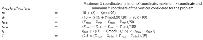
Table 1.Formulae used to generate parameters for team orienteering problem with variable profits (TOPVP) instances.
XmaxXminYmaxYmin =
MaximumXcoordinate, minimumXcoordinate, maximumYcoordinate and minimumYcoordinate of the vertices considered for the problem
pi = 10+(Xi+Yimod90)
ai = (10+(((Xi+Yimod20)/20)×90))/100
rmax = (Xmax−Xmin+Ymax−Ymin)/50
rmin = (Xmax−Xmin+Ymax−Ymin)/100
ri = rmin+(((Xi+Yimod15)/15)×(rmax−rmin))
T = (2.5×(Xmax−Xmin+Ymax−Ymin))/|P|
The TSP instances used are kroA100, kroB100, kroC100, kroA200 and kroB200, which are obtained from the TSPLIB. The number in the instance’s name represents the number of vertices. The first vertex from the data file is set as the depot. The edge coststijare determined from the ver-tex coordinates using Euclidean distance. Note that the 200-verver-tex instances are extensions of the 100-vertex instances, with the first 100 vertices being the same.
The OPVP instances are then used to generate the TOPVP instances. This is done by taking the one-path OPVP and dividing the time budget by the number of paths in TOPVP (Chao, Golden, and Wasil1996a). In other words, the accumulative total time budget for the paths in TOPVP is the same as the time budget for OPVP. Table1summarizes the formulae used to generate the parameters from the vertex coordinates.
Verification and validation of the ILS algorithm were conducted using the CPLEX solver to solve for the optimal solution for small test instances. The objective is to compare the optimal solution of the instances with that of ILS. The optimality gap for the ILS solutions can be determined, although this is only for small test instances.
The factors tested in the verification and validation experiments are the number of vertices|V|, number of paths|P|and time budget for each pathT. Since the test instances from TSPLIB are in sets of 100 vertices (kroA100, kroB100 and kroC100) and 200 vertices (kroA200 and kroB200), solving to optimality using all the test instances with such significant sizes will be beyond computational reach. As such, to reduce the size of the experiments, only the initial 15 vertices from each test instance are used, and experiments for five, 10 and 15 vertices are conducted. In addition, the number of paths
|P|tested for each test instance is one, two and three. The solver CPLEX 12.6.2 was used to solve the TOPVP on a computer with an Intel Xeon E5-1603 CPU at 2.80 GHz and 16 GB RAM.
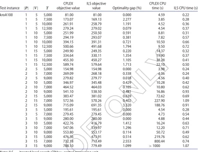
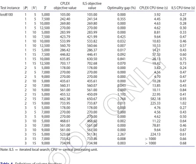
The objective value of the solutions obtained from CPLEX and ILS are recorded in Tables2and3. Part of the verification process involves checking whether the objective values from ILS have exceeded the objective value of the optimal solution and, as can be observed, these objective values do not exceed the optimal objective value. In addition, the solutions are checked to ensure that the paths remained feasible. Furthermore, the maximum optimality gap for all the experiments conducted is 3.32%, which is an acceptable value for small instances.
For the time budget assigned for each path/vehicle, arbitrary values are picked for the verification and validation experiments. This is because by evaluating ILS over a comprehensive range of time budget values, the verification and validation process can be more credible. To illustrate, the edge costs calculated from the test instances can go up to about 3000 time units. For experiments with only five vertices considered or 5000 time units allocated for each vehicle, the optimality gap is likely to be 0%. This can be attributed to the elimination of vertices that require more than 2500 time units when visiting from the depot. These vertices are eliminated from consideration since they cannot be visited without exceeding the time budget. As such, the reduction in the number of vertices considered resulted in ILS being more likely to converge to the optimal solution.
562 563 564 565 566 567 568 569 570 571 572 573 574 575 576 577 578 579 580 581 582 583 584 585 586 587 588 589 590 591 592 593 594 595 596 597 598 599 600 601 602 603 604 605 606 607 608 609 610 611 612
Table 2.Validation results for kroA100.
Test instance |P| |V| T
CPLEX objective value
ILS objective
value Optimality gap (%)
CPLEX CPU
time (s) ILS CPU time (s)
kroA100 1 5 5,000 81.00 81.00 0.000 4.59 0.22
1 5 7,500 173.07 169.13 2.277 3.85 0.28
1 5 10,000 261.91 258.79 1.191 4.52 0.36
1 5 12,500 279.24 279.02 0.079 4.54 0.37
1 10 5,000 251.99 250.50 0.591 8.81 0.31
1 10 7,500 294.19 293.07 0.381 7.82 0.57
1 10 10,000 394.15 391.31 0.721 10.50 0.66
1 10 12,500 500.66 491.68 1.794 9.50 0.72
1 15 5,000 249.90 249.35 0.220 14.37 0.32
1 15 7,500 334.64 330.11 1.354 19.90 0.37
1 15 10,000 455.30 450.27 1.105 38.28 0.41
1 15 12,500 589.74 579.64 1.713 22.10 0.50
2 5 5,000 154.98 154.98 0.000 3.98 0.24
2 5 7,000 269.09 268.18 0.338 4.06 0.24
2 5 9,000 279.82 279.77 0.018 4.56 0.40
2 10 5,000 346.97 345.48 0.429 10.28 0.42
2 10 7,000 464.52 464.03 0.105 10.80 0.62
2 10 9,000 541.10 538.50 0.481 16.86 0.93
2 15 5,000 383.47 381.02 0.639 72.62 0.69
2 15 7,000 572.56 570.26 0.402 227.90 1.09
2 15 9,000 715.09 691.35 3.320 188.76 0.91
3 5 5,000 195.61 195.61 0.000 4.54 0.28
3 5 7,000 279.45 279.45 0.000 4.73 0.54
3 5 9,000 280.00 280.00 0.000 4.88 0.44
3 10 5,000 422.76 416.79 1.412 16.24 0.63
3 10 7,000 547.06 539.97 1.296 12.20 0.71
3 10 9,000 553.80 553.17 0.114 50.72 0.49
3 15 5,000 476.36 473.91 0.514 219.76 0.62
3 15 7,000 732.18 713.49 2.553 800.44 0.74
3 15 9,000 788.10 779.49 1.099 >1000 1.07
Note: ILS=iterated local search; CPU=central processing unit.
because given a larger time budget, the paths in the solution will be longer and the maximum allow-able passes made at each path will be higher. Thus, setting a larger time budget is likely to be beyond computational reach.
5.2. Computational results
In this section, experiments were conducted for the full range of vertices using the test instances kroA100, kroB100, kroC100, kroA200 and kroB200. Results obtained from CPLEX after 1000 s of computational time were compared with the results obtained by ILS. The objective is to evaluate the performance of the ILS algorithm using the best upper bound as well as the best feasible integer solution obtained by CPLEX.
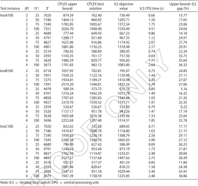
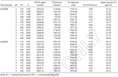
The numbers of vertices used for kroA100, kroB100 and kroC100 instances are varied at 25, 50, 75 and 100, using the initial vertices for each instance. The numbers of vertices used for kroA200 and kroB200 instances are varied at 125, 150, 175 and 200 to avoid repetition of computational results due to using the same initial vertices for each instance. Experiments are conducted for two-, three- and four-path TOPVPs. The definitions of the column headings are given in Table4. The results for the kroA100, kroB100 and kroC100 instances are presented in Table5. Table6presents the results for the larger instances kroA200 and kroB200.
613 614 615 616 617 618 619 620 621 622 623 624 625 626 627 628 629 630 631 632 633 634 635 636 637 638 639 640 641 642 643 644 645 646 647 648 649 650 651 652 653 654 655 656 657 658 659 660 661 662 663
Table 3.Validation results for kroB100.
Test instance |P| |V| T
CPLEX objective value
ILS objective
value Optimality gap (%) CPLEX CPU time (s) ILS CPU time (s)
kroB100 1 5 5,000 103.00 103.00 0.000 3.92 0.27
1 5 7,500 242.40 241.54 0.355 4.45 0.28
1 5 10,000 269.80 269.80 0.000 4.63 0.28
1 5 12,500 270.00 270.00 0.000 4.62 0.30
1 10 5,000 283.99 283.99 0.000 8.81 0.33
1 10 7,500 423.79 421.99 0.425 9.64 0.47
1 10 10,000 533.99 533.82 0.032 10.83 0.46
1 10 12,500 560.70 560.66 0.007 10.53 0.57
1 15 5,000 286.42 286.37 0.017 14.21 0.43
1 15 7,500 446.82 446.41 0.092 57.53 0.60
1 15 10,000 635.85 630.50 0.841 26.13 0.75
1 15 12,500 703.17 702.68 0.070 19.42 0.73
2 5 5,000 178.00 178.00 0.000 3.82 0.24
2 5 7,000 270.00 270.00 0.000 4.56 0.47
2 5 9,000 270.00 270.00 0.000 4.70 0.47
2 10 5,000 435.61 435.61 0.000 10.28 0.47
2 10 7,000 560.31 560.07 0.043 13.85 0.43
2 10 9,000 561.00 561.00 0.000 10.11 0.84
2 15 5,000 455.52 450.09 1.192 22.95 0.41
2 15 7,000 662.38 650.67 1.768 582.18 0.93
2 15 9,000 733.95 733.87 0.011 225.33 1.02
3 5 5,000 178.00 178.00 0.000 4.76 0.27
3 5 7,000 270.00 270.00 0.000 4.56 0.43
3 5 9,000 270.00 270.00 0.000 4.62 0.50
3 10 5,000 468.61 468.60 0.002 11.22 0.64
3 10 7,000 561.00 561.00 0.000 78.81 0.46
3 10 9,000 561.00 561.00 0.000 9.64 0.67
3 15 5,000 523.68 511.81 2.267 224.13 0.61
3 15 7,000 733.42 733.36 0.008 >1000 0.66
3 15 9,000 734.99 734.98 0.003 >1000 0.68
[image:13.493.47.448.65.400.2]Note: ILS=iterated local search; CPU=central processing unit.
Table 4.Definitions of column headings.
CPLEX upper bound :Best upper bound obtained by CPLEX at 1000 s
CPLEX best solution :Objective value of the best solution obtained by CPLEX at 1000 s TOPVP objective value :Objective value of the ILS
TOPVP CPU time (s) :Computational time required for the ILS
Upper bound–TOPVP gap (%) :Percentage deviation of the ILS’s objective value from CPLEX upper bound
Note: TOPVP=team orienteering problem with variable profits; ILS=iterated local search; CPU=central processing unit.
intensive. In addition, the computational time for experiments with comparatively more paths is gen-erally lower. This can be attributed to the time budget allocated for each path being lower than in experiments with fewer paths. Since the time budget is lower, the paths constructed are shorter and the maximum number of passes allowed for each vertex is lower. Thus, the possibility of achieving improvement from the local search component of ILS is lower. Hence, ILS is able to converge to a solution using fewer iterations in the improvement phases.
Although the gap between the solution obtained from ILS and the upper bound is considerably large, it can be reasonably justified. Given the termination time being set at 1000 s, there is already a large optimality gap between the upper bound and the solution obtained by CPLEX. Hence, the actual optimality gap for ILS is likely to be smaller than the gap reported in Tables5and6. This is seen in the kroB100 instance with|V| =4,|P| =25 andT =3359, where the optimal solution was obtained by CPLEX and the optimality gap for ILS is only 0.22%.
664 665 666 667 668 669 670 671 672 673 674 675 676 677 678 679 680 681 682 683 684 685 686 687 688 689 690 691 692 693 694 695 696 697 698 699 700 701 702 703 704 705 706 707 708 709 710 711 712 713 714
Table 5.Computational results for kroA100, kroB100 and kroC100.
Test instance |P| |V| T
CPLEX upper bound
CPLEX best solution
ILS objective
value ILS CPU time (s)
Upper bound–ILS gap (%)
kroA100 2 25 7020 874.39 762.40 736.49 0.66 15.77
2 50 7186 1464.12 868.92 1205.71 1.50 17.65
2 75 7240 1783.85 1005.67 1372.54 1.75 23.06
2 100 7351 2026.70 1408.40 1539.49 4.51 24.04
3 25 4680 777.44 649.45 667.23 0.86 14.18
3 50 4791 1288.17 921.60 967.35 1.12 24.91
3 75 4827 1625.96 916.86 1174.92 2.07 27.74
3 100 4901 1881.80 1150.23 1318.98 2.17 29.91
4 25 3510 746.92 588.89 580.05 0.74 22.34
4 50 3593 1143.35 761.17 757.50 0.64 33.75
4 75 3620 1486.59 829.77 956.83 1.77 35.64
4 100 3673 1701.83 982.12 1083.80 2.64 36.32
kroB100 2 25 6718 1057.95 702.81 795.07 0.75 24.85
2 50 7051 1550.25 1122.16 1129.98 1.44 27.11
2 75 7275 1934.81 1189.21 1410.98 2.34 27.07
2 100 7391 2519.20 1548.81 1837.54 5.79 27.06
3 25 4478 589.34 573.72 570.74 0.85 3.16
3 50 4701 1216.24 1042.29 1017.78 1.49 16.32
3 75 4850 1707.65 1285.83 1344.68 1.03 21.26
3 100 4927 2319.70 1559.52 1731.71 1.97 25.35
4 25 3359 520.67 520.67 519.50 0.79 0.22
4 50 3526 1137.17 951.78 942.26 1.47 17.14
4 75 3638 1605.68 1076.38 1193.96 1.33 25.64
4 100 3696 2252.69 1207.40 1514.31 1.85 32.78
kroC100 2 25 7020 832.62 735.28 689.65 0.71 17.17
2 50 7186 1418.87 1008.78 1118.80 1.63 21.15
2 75 7240 1930.83 1238.18 1368.79 2.56 29.11
2 100 7345 2285.38 1240.78 1665.63 3.90 27.12
3 25 4680 794.99 627.43 586.49 0.69 26.23
3 50 4791 1244.62 953.44 973.19 1.73 21.81
3 75 4827 1762.39 1114.87 1233.01 2.48 30.04
3 100 4897 2151.57 1157.68 1497.63 2.73 30.39
4 25 3510 557.57 517.37 491.55 0.83 11.84
4 50 3593 1081.96 828.61 818.23 1.58 24.38
4 75 3620 1547.31 951.18 1029.44 2.40 33.47
4 100 3673 1941.39 1158.59 1225.85 2.48 36.86
Note: ILS=iterated local search; CPU=central processing unit.
instances, the gaps for the experiments using only 25 vertices are considerably small, 3.16% and 0.22%, respectively. The reason for this is two-fold: the number of vertices is only 25, and the time budgets allocated for the three- and four-path experiments are relatively low. As such, the number of feasible vertices in the time budget constraint is small, enabling ILS to reach a near-optimal solution. On the other hand, for experiments with more vertices available, ILS is unable to achieve a comparable small gap. By the same argument, the number of feasible vertices for ILS to consider is large, which explains the much larger gap reported.
715 716 717 718 719 720 721 722 723 724 725 726 727 728 729 730 731 732 733 734 735 736 737 738 739 740 741 742 743 744 745 746 747 748 749 750 751 752 753 754 755 756 757 758 759 760 761 762 763 764 765
Table 6.Computational results for kroA200 and kroB200.
Test instance |P| |V| T
CPLEX upper bound
CPLEX best solution
ILS objective
value ILS CPU time (s)
Upper bound–ILS gap (%)
kroA200 2 125 7345 2556.54 1126.84 1755.72 3.90 31.32
2 150 7380 2826.82 1267.49 1914.66 7.17 32.27
2 175 7380 2994.77 466.22 2036.53 5.21 32.00
2 200 7380 3117.18 155.99 2111.68 8.94 32.26
3 125 4897 2362.61 1091.55 1687.18 3.34 28.59
3 150 4920 2638.86 1072.10 1722.68 4.77 34.72
3 175 4920 2790.47 858.58 1860.15 4.89 33.34
3 200 4920 2906.92 247.89 1917.95 4.97 34.02
4 125 3673 2263.87 1136.59 1405.30 2.17 37.92
4 150 3690 2388.89 1081.03 1498.14 2.94 37.29
4 175 3690 2538.22 1235.60 1595.99 3.18 37.12
4 200 3690 2700.82 734.89 1630.20 3.70 39.64
kroB200 2 125 7391 2727.64 1091.29 1905.82 5.19 30.13
2 150 7391 2957.56 1357.81 2048.07 6.83 30.75
2 175 7391 3102.08 1319.55 2119.59 11.95 31.67
2 200 7401 3320.49 948.71 2233.36 8.82 32.74
3 125 4927 2475.03 1530.28 1802.51 4.08 27.17
3 150 4927 2675.39 1496.86 1920.98 3.74 28.20
3 175 4927 2833.15 1329.10 2102.80 5.33 25.78
3 200 4934 3093.34 617.07 2116.00 7.36 31.59
4 125 3696 2393.64 1271.46 1605.69 2.54 32.92
4 150 3696 2617.37 1486.56 1813.00 4.63 30.73
4 175 3696 2828.17 1298.20 1853.34 3.67 34.47
4 200 3701 3001.25 897.02 1976.09 3.67 34.16
Note: ILS=iterated local search; CPU=central processing unit.
6. Conclusion
A variant of the OP, namely the TOPVP is introduced. For the TOPVP, multiple paths are involved in collecting scores which are dependent on the time spent at the visited vertices. In this article, the TOPVP is formulated as a mathematical programming model that could be extended to other models. One of the future plans for extending the model is to include the correlated effect among vertices (in the context of the tourist trip design problem). The objective function for this extended model will consist of two components: the total of the collected scores from visited nodes and a quadratic score function that captures spatial correlations among nodes (Yu, Schwager, and Rus2014).
An ILS algorithm has been developed to solve the modified benchmark TOPVP instances. The results obtained from solving some modified benchmark instances by ILS are compared with those obtained by the CPLEX solver, which is able to solve small instances to optimality. For these small instances ranging up to 15 vertices, ILS is able to achieve optimality in several experiments using considerably shorter computational time. ILS is then applied to larger instances ranging up to 200 vertices. While the computational time needed for ILS is low, the gap between the ILS results and the upper bound obtained by CPLEX solver after 1000 s is still considerably small, and the ILS is able to obtain better solutions than the CPLEX solver after 1000 s in most of the larger instances. However, the development of a more effective heuristic incorporating more advanced operators to achieve a smaller optimality gap is a possible direction for future research.
766 767 768 769 770 771 772 773 774 775 776 777 778 779 780 781 782 783 784 785 786 787 788 789 790 791 792 793 794 795 796 797 798 799 800 801 02 803 804 805 806 807 808 809 10 811 812 813 814 815 816
Finally, the idea of using stronger mathematical programming models and exact algorithms, such as the branch-and-cut approach in Erdoğan and Laporte (2013), to generate better upper bound values will be considered for future work as well.
Disclosure statement
No potential conflict of interest was reported by the authors.
ORCID
Graham Kendall http://orcid.org/0000-0003-2006-5103
References
Archetti, C., N. Bianchessi, M. G. Speranza, and A. Hertz.2014. “The Split Delivery Capacitated Team Orienteering Problem.”Networks63 (1): 16–33.
Archetti, C., A. Hertz, and M. G. Speranza.2007. “Metaheuristics for the Team Orienteering Problem.”Journal of Heuristics13 (1): 49–76.
Boussier, S., D. Feillet, and M. L. Gendreau.2007. “An Exact Algorithm for Team Orienteering Problems.”4OR5 (3): 211–230.
Chao, I., B. Golden, and E. Wasil.1996a. “A Fast and Effective Heuristic for the Orienteering Problem.”European Journal of Operational Research88 (3): 475–489.
Chao, I., B. Golden, and E. Wasil.1996b. “The Team Orienteering Problem.”European Journal of Operational Research 88 (3): 464–474.
Dang, D.-C., R. N. Guibadj, and A. Moukrim.2013. “An Effective PSO-Inspired Algorithm for the Team Orienteering Problem.”European Journal of Operational Research229 (2): 332–344.
Divsalar, A., P. Vansteenwegen, and D. Cattrysse.2013. “A Variable Neighborhood Search Method for the Orienteering Problem with Hotel Selection.”International Journal of Production Economics145 (1): 150–160.
Dueck, G.1993. “New Optimization Heuristics: The Great Deluge Algorithm and the Record-to-Record Travel.”Journal of Computational Physics104 (1): 86–92.
El-Hajj, R., D.-C. Dang, and A. Moukrim.2016. “Solving the Team Orienteering Problem with Cutting Planes.” Computers & Operations Research74: 21–30.
Erdoğan, G., and G. Laporte.2013. “The Orienteering Problem with Variable Profits.”Networks61 (2): 104–116. Ferreira, J., A. Quintas, and J. A. Oliveira.2014. “Solving the Team Orienteering Problem: Developing a Solution Tool
Using a Genetic Algorithm Approach.” InSoft Computing in Industrial Applications. Vol. 223, edited by V. Snášelet al., 365–375. Springer.
0
Gendreau, M., G. Laporte, and F. Semet.1997. “The Covering Tour Problem.”Operations Research45 (4): 568–576. Golden, B. L., Q. Wang, and L. Liu.1987. “The Orienteering Problem.”Naval Research Logistics34 (3): 307–318. Gunawan, A., H. C. Lau, and P. Vansteenwegen.2016. “Orienteering Problem: A Survey of Recent Variants, Solution
Approaches and Applications.”European Journal of Operational Research255 (2): 315–332.
Harvey, W. D., and M. L. Ginsberg.1995. “Limited Discrepancy Search.” Proceedings of the 14th international joint conference on artificial intelligence, Canada, August 20–25, 607–615.
Heidelberg University.n.d. “TSPLIB.” Retrieved from Discrete and Combinatorial Optimization:http://comopt.ifi. uni-heidelberg.de/software/TSPLIB95/index.html.
2
Ke, L., L. Zhai, J. Li, and F. T. S. Chan.2015. “Pareto Mimic Algorithm: an Approach to the Team Orienteering Problem.” Omega61: 155–166.
Keshtkaran, M., K. Ziarati, A. Bettinelli, and D. Vigo. 2016. “Enhanced Exact Solution Methods for the Team Orienteering Problem.”International Journal of Production Research54 (2): 591–601.
Laporte, G., and S. Martello.1990. “The Selective Travelling Salesman Problem.”Discrete Applied Mathematics26 (2–3): 193–207.
Lourenço, H. R., O. C. Martin, and T. Stützle.2003. “Iterated Local Search.” InHandbook of Metaheuristics, edited by F. Glover, and G. A. Kochenberger, 320–353. Springer.
Palomo-Martinez, P. J., M. A. Salazar-Aquilar, G. Laporte, and A. Langevin.2017. “A Hybrid Variable Neighborhood Search for the Orienteering Problem with Mandatory Visits and Exclusionary Constraints.”Computers & Operations Research78: 408–419.
Souffriau, W., P. Vansteenwegen, J. Vertommen, G. Vanden Berghe, and D. Van Oudheusden.2008. “A Personalized Tourist Trip Design Algorithm for Mobile Tourist Guides.”Applied Artificial Intelligence22 (10): 964–985. Tsiligirides, T.1984. “Heuristic Methods Applied to Orienteering.”Journal of the Operational Research Society35 (9):
817 818 819 820 821 822 823 824 825 826 827 828 829 830 831 832 833 834 835 836 837 838 839 840 841 842 843 844 845 846 847 848 849 850 851 852 853 854 855 856 857 858 859 860 861 862 863 864 865 866 867
Vansteenwegen, P., W. Souffriau, and D. Van Oudheusden.2011. “The Orienteering Problem: A Survey.”European Journal of Operational Research209 (1): 1–10.
Vansteenwegen, P., W. Souffriau, G. Vanden Berghe, and D. Van Oudheusden. 2009. “A Guided Local Search Metaheuristic for the Team Orienteering Problem.”European Journal of Operational Research196 (1): 118–127. Yu, J., M. Schwager, and D. Rus.2014. “Correlated Orienteering Problem and its Application to Informative Path