Sparse generalized kernel modeling for nonlinear systems

Sparse Generalized Kernel Modeling for Nonlinear Systems

S. Chen, X. Hong, X.X. Wang and C.J. Harris

Abstract— A generalized kernel modeling approach is pro-posed for identification of discrete-time nonlinear systems. Each kernel regressor in the generalized kernel model has an individually fitted diagonal covariance matrix which is deter-mined by maximizing the correlation between the regressor and training data. A state-of-the-art construction algorithm based on orthogonal least squares regression with leave-one-out test statistic and local regularization is applied to select a parsimonious generalized kernel model from the full regression matrix. The effectiveness of the proposed nonlinear modeling approach is demonstrated by the experimental results involving one simulated system and two real data sets.

I. INTRODUCTION

The class of the orthogonal least squares (OLS) algo-rithms [1]–[6] provides an effective construction method that is capable of producing parsimonious linear-in-the-weights nonlinear models with excellent generalization performance. Alternatively, the state-of-the-art sparse kernel modeling techniques, such as the support vector machine and relevant vector machine [7]–[12], have been gaining popularity in data modeling applications. These existing sparse regression modeling techniques typically employ a single common kernel variance for all the regressors. The value of this common kernel variance has a crucial influence on the sparsity level and generalization capability of the resulting model, and it has to be determined via cross validation. For example, in [3] a genetic algorithm is applied to determine the appropriate common kernel variance through optimizing the model generalization performance.

We propose a generalized kernel model, in which each kernel regressor has an individually tuned diagonal covari-ance matrix. This generalized kernel model has the potential of enhancing modeling capability and producing sparser models. The difficult issue is how to determine these kernel covariance matrices. Since the correlation between a kernel regressor and the training data defines the “similarity” be-tween the regressor and training data, we can “shape” the re-gressor by adjusting the associated kernel covariance matrix in order to maximize the absolute value of this correlation function. We employ the repeated weighted boosting search (RWBS) algorithm [13] to perform kernel covariance fitting. This algorithm is a guided random search method having its root from boosting optimization [14]-[17]. The determination of kernel covariance matrices provides the pool of regressors,

S. Chen and C.J. Harris are with School of Electronics and Computer Science, University of Southampton, Southampton SO17 1BJ, U.K. E-mails:

{sqc,chj}@ecs.soton.ac.uk

X. Hong is with Department of Cybernetics, University of Reading, Reading, RG6 6AY, U.K. E-mail: [email protected]

X.X. Wang is with Neural Computing Research Group, Aston University, Birmingham B4 7ET, U.K. E-mail: [email protected]

from which a sparse subset model can be selected using a standard kernel model construction approach.

We adopt the OLS algorithm with the leave-one-out (LOO) test score and local regularization [6], referred to as the LROLS with LOO for short, to select a sparse generalized kernel model. This construction algorithm selects significant regressors by directly maximizing model generalization ca-pability, without resorting to use a separate validation data set. The algorithm is computationally efficient and can pro-duce very parsimonious models due to local regularization that enforces sparse solutions. Moreover, the model building process is automatic without the need for the user to specify some additional termination criterion. The effectiveness of the propose generalized kernel modeling approach is illus-trated by three nonlinear system identification examples.

II. GENERALIZED KERNEL MODELING

Consider a general discrete stochastic nonlinear system represented by [18]:

yk = fs(yk−1,· · ·, yk−ny, uk−1,· · ·, uk−nu;θ) +ek

= fs(xk;θ) +ek (1)

where uk and yk are the system input and output vari-ables, respectively, nu and ny are positive integers rep-resenting the known lags in uk and yk, respectively, the observation noise ek is uncorrelated with zero mean,xk = [yk−1· · ·yk−ny uk−1· · ·uk−nu]T denotes the system input

vector with a known dimension n=ny+nu,fs(•) is the unknown system mapping, andθ is an unknown parameter vector associated with an appropriate model structure. The system model (1) is to be identified from an N-sample system observational data setDN ={xk, yk}Nk=1.

We will model the unknown dynamical process (1) by using a generalized kernel regression model of the form:

yk= ˆyk+k= N

i=1

θigi(xk) +k=gT(k)θ+k (2)

where yˆk denotes the model output given the input xk,k is the modeling error, θ = [θ1 θ2· · ·θN]T is the model weight vector, and g(k) = [g1(xk) g2(xk)· · ·gN(xk)]T is the regressor vector at the point xk. The model kernel regressors are given by

gi(x) =ϕ(x−xi)T_Σ−1

i (x−xi)

(3)

withϕ(•)being a chosen kernel function. The kernel centers are placed directly on the training inputsxi, but each kernel regressor has a kernel covariance matrix taking the form of

Proceedings of the

44th IEEE Conference on Decision and Control, and the European Control Conference 2005

Seville, Spain, December 12-15, 2005

i i,1 i,n N model (2) can be written in the matrix form as

y=Gθ+ (4)

by defining y = [y1 y2· · ·yN]T, = [1 2· · ·N]T and G= [g1 g2· · ·gN]with gi= [gi(x1) gi(x2)· · ·gi(xN)]T, 1≤i≤N. Note thatgk is thekth column of the regression matrixG, whileg(k)is the kth row ofG.

Let an orthogonal decomposition of G be G = ΦA, where

A=

⎡ ⎢ ⎢ ⎢ ⎢ ⎣

1 a1,2 · · · a1,N 0 1 . .. ... ..

. . .. ... aN−1,N

0 · · · 0 1

⎤ ⎥ ⎥ ⎥ ⎥

⎦ (5)

andΦ= [φ₁φ₂· · ·φ_N]satisfyingφT_iφ_j= 0, ifi=j. The regression model (4) can alternatively be expressed as

y=Φw+ (6)

where the weight vector w= [w1 w2· · ·wN]T, defined in the new spaceΦ, satisfy the triangular systemAθ=w. The space spanned by the original model bases gi,1≤i≤N, is identical to the space spanned by the orthogonal basesφ_i, 1≤i≤N, andyˆk can equivalently be expressed by

ˆ

yk=φT(k)w (7) where φ(k) = [φk,1φk,2· · ·φk,N]T is thekth row ofΦ.

III. SPARSE MODEL CONSTRUCTION ALGORITHM The objective of sparse modeling is to construct a subset model consisting of Ns (N) significant regressors from the full model defined in (2), which can adequately model the underlying system (1).

A. Determination of the full regression matrix

To specify the pool of regressors or the full regression matrixG, we need to determine all the associated diagonal covariance matricesΣi,1≤i≤N. The correlation between a regressor gi and the training data, defined by

C(Σi) =

yT_gi

yT_ygT

igi

(8)

represents the “similarity” between gi and y. We should choose Σi so that |C(Σi)| is maximized. It can easily be shown that this is a good strategy to specify the pool of regressors. Let us first define the least squares cost or mean square error (MSE) associated with anm-term model as

Sm= 1

N

N

k=1

(yk−yˆk)2 (9)

Obviously S0 = yT_{y/N = y}2_{/N. Assuming that gi is}

selected to form a one-term model, the associated reduction in the MSE value can be shown to be ∆S = S0−S1 =

yT_gi2_/gT

i gi, which can be rewritten as

∆S=yT_y

yT_gi2 (yTy)gT

igi

=y2_|C(Σi)|2

(10)

maximum reduction in the MSE value.

We apply the RWBS algorithm [13] to perform the associ-ated optimization tasks for fitting kernel covariance matrices. The RWBS algorithm is a simple yet efficient global search algorithm that adopts some ideas from boosting [14]-[17]. The RWBS optimizer is given in Appendix. Once the full regression matrix G has been designed, the LROLS with LOO [6] can be used to select a subset model.

B. Efficient subset model selection

The weight vector wis obtained as the regularized least squares solution obtained by minimizing the cost

JR(w,λ) =T₊ N

i=1

λiwi2 (11)

where λ = [λ1 λ2· · ·λN]T is the regularization parameter vector, which is optimized based on the evidence procedure with the iterative updating formulas [5],[6]

λnew

i =

γold

i

N−γold T

w2

i

, 1≤i≤N (12)

where

γi= φ T

iφi

λi+φTiφi

and γ=

N

i=1

γi (13)

Usually a few iterations (typically less than 10) are sufficient to find a local optimalλ. The Bayesian interpretation of the criterion JR(w,λ) together with the full derivation of the updating formulas (12) and (13) can be found in [5].

A forward selection procedure is used to construct a sparse model by incrementally minimizing the LOO test score. Assume that anm-term model is selected from the full model (6). The LOO test error [19]-[22], denoted as (_km,−k), for the selected m-term model can be shown to be [4],[6]

(m,−k)

k =

(m)

k /η

(m)

k (14)

where (_km) is the m-term modeling error and η(_km) is the associated LOO error weighting given by

η(m)

k = 1−

m

i=1

φ2

k,i

φT

iφi+λi

(15)

The mean square LOO error for the model with a sizemis defined by

Jm=E

(m,−k)

k

2

= 1

N

N

k=1

(m)

k

2

η(m)

k

2 (16)

This LOO statistic is a measure of the model generalization performance and it can be computed efficiently because(_km) and η(_km) can be calculated recursively according to

(m)

k =yk−

m

i=1

-1 -0.5 0 0.5 1

200 220 240 260 280 300

System output/Model prediction

sample

(a)

-0.2 -0.1 0 0.1 0.2

200 220 240 260 280 300

Model prediction error

sample

(b)

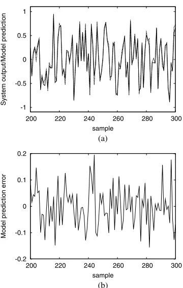
Fig. 1. Performance of the 15-term generalized Gaussian kernel model for the simulated system: (a) model prediction (dashed) superimposed on noisy system output (solid), and (b) model prediction error.

η(m)

k =η

(m−1)

k −

φ2

k,m

φT

mφm+λm

(18)

respectively. The idea of delete-one cross validation and the associated LOO test error are explained in [4],[6].

The subset model selection procedure can be carried as follows: at themth stage of the selection procedure, a model term is selected among the remaining m to N candidates if the resulting m-term model produces the smallest LOO test score Jm. It has been shown in [4] that the LOO statistic Jm is convex with respect to the model size m. That is, there exists an “optimal” model sizeNssuch that for

m≤NsJmdecreases asmincreases while form≥Ns+1

Jm increases asm increases. Thus the selection procedure is automatically terminated with an Ns-term model when

JNs+1 > JNs, without the need for the user to specify a

separate termination criterion. The details of the iterative procedure for constructing a sparse model based on the LROLS with LOO can be found in [6].

IV. MODELING EXAMPLES

Three examples were used to demonstrate the effectiveness of the proposed model construction algorithm.

Example 1. This was the system considered in [23]. The underlying dynamic system was governed by

zk=

zk−1zk−2zk−3uk−2(zk−3−1) +uk−1

1 +z2

k−2+zk2−3

(19)

-1 -0.5 0 0.5 1

200 220 240 260 280 300

System noise-free output/Model iterative

sample

(a)

-0.2 -0.1 0 0.1 0.2

200 220 240 260 280 300

Model iterative error

sample

(b)

Fig. 2. Performance of the 15-term generalized Gaussian kernel model for the simulated system: (a) iterative model output (dashed) superimposed on noise-free system output (solid), and (b) iterative model error.

where the system input uk was a random signal uniformly distributed in the interval[−1, 1]. The noisy system output was given byyk=zk+ek, where the noiseekwas Gaussian distributed with zero mean and standard deviation 0.05. Four hundred noisy samples were generated. The first 200 data points were used for training, and the other 200 samples were used for model validation. The generalized Gaussian kernel model with the input vector

xk= [yk−1yk−2 yk−3uk−1uk−2]T (20)

was used to construct a model from the noisy training set. The N = 200 candidates’ kernel covariance matrices were first determined by the RWBS algorithm, and the LROLS with LOO then selected a 15-term generalized Gaussian kernel model. The MSE values of this model over the training and testing sets were 0.003244 and 0.005195, respectively. The model prediction yˆk and prediction error

k = yk −yˆk over the first 100 data points of the test set are depicted in Fig. 1. The constructed 15-term model was also used to iteratively generate the model output according to yˆd,k = fm(ˆxd,k) with the input ˆxd,k = [ˆyd,k−1 ˆyd,k−2 yˆd,k−3 uk−1 uk−2]T, where fm(•) denotes

the model mapping. The iterative model output yˆd,k and iterative error, defined by ˆd,k = zk−yˆd,k, are shown in Fig. 2 over the first 100 data points of the test set.

2.5 3 3.5 4 4.5

0 50 100 150 200 250 300 350 400

System output/Model prediction

sample

(a)

-0.1 -0.05 0 0.05 0.1

0 50 100 150 200 250 300 350 400

Model prediction error

sample

(b)

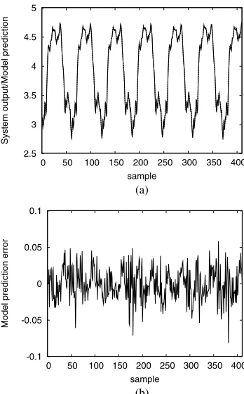
Fig. 3. Performance of the 15-term generalized Gaussian kernel model for the engine data set: (a) model prediction (dashed) superimposed on system output (solid), and (b) model prediction error.

ious existing kernel regression techniques were used in [6] to fit a thin-plate-spline regression model for this system, and the best result obtained had a 31-term thin-plate-spline regression model with the MSE values of 0.003192 and 0.005892 over the training and validation sets, respectively.

Example 2. This example constructed a model representing the relationship between the fuel rack position (input uk) and the engine speed (output yk) for a Leyland TL11 turbocharged, direct injection diesel engine operated at a low engine speed. Detailed system description and experimental setup can be found in [24]. The data set contained 410 samples. The first 210 data points were used in training and the last 200 points in model validation. The previous results [5],[6] had shown that when fitting a Gaussian kernel model with a single common variance, σ2 = 1.69 was the optimal value for this kernel variance, and the model input was given by xk = [yk−1 uk−1 uk−2]T. Various kernel

modeling techniques were employed in [6] to fit this data set, and the best Gaussian kernel model constructed consisted of 22 terms. The MSE values of this model over the training and validation sets were0.000453and0.000490, respectively.

The proposed modeling approach was applied to construct a generalized Gaussian kernel model, yielding a 15-term subset model. The MSE values of this model were0.000482 over the training set and0.000496 over the validation set, respectively. The model prediction yˆk and prediction error

k = yk −yˆk generated by this model are illustrated in Fig. 3. This obtained 15-term model was used to iteratively

2.5 3 3.5 4 4.5

0 50 100 150 200 250 300 350 400

System output/Model iterative

sample

(a)

-0.15 -0.1 -0.05 0 0.05 0.1 0.15

0 50 100 150 200 250 300 350 400

Model iterative error

sample

(b)

Fig. 4. Performance of the 15-term generalized Gaussian kernel model for the engine data set: (a) iterative model output (dashed) superimposed on system output (solid), and (b) iterative model error.

generate the model output yˆd,k = fm(ˆxd,k) with the input vector xˆd,k = [ˆyd,k−1 uk−1 uk−2]T. The iterative model

output yˆd,k and the iterative model error d,k =yk−yˆd,k, are depicted in Fig. 4.

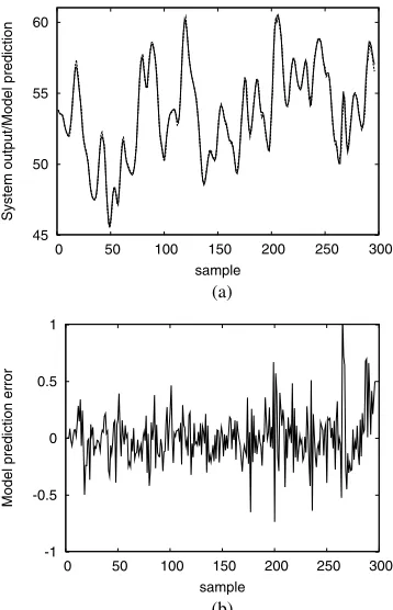
Example 3. The gas furnace data set (Series J in [25]) contained 296 pairs of input-output points, where the input

uk was the coded input gas feed rate and the output yk was the CO2 concentration. All the 296 data points were

used in training, with the model input vector defined by xk = [yk−1 yk−2 yk−3 uk−1 uk−2 uk−3]T. The previous experiments had found out that the existing state-of-the-art kernel regression techniques failed to fit a Gaussian kernel regression model using a common kernel variance [6]. Various existing kernel modeling methods were used in [6] to fit a thin-plate-spline regression model, and the best thin-plate-spline model obtained contained 28 terms with the training MSE0.053306.

By adopting the proposed generalized kernel model ap-proach, a 21-term generalized Gaussian kernel model was identified with the training MSE 0.053452. The model prediction and prediction error generated by this 21-term generalized Gaussian kernel model are shown in Fig. 5. The obtained model was also used to iteratively produce the model output yˆd,k = fm(ˆxd,k) given the inputxd,kˆ = [ˆyd,k−1 yˆd,k−2 yˆd,k−3 uk−1 uk−2 uk−3]T. The iterative

model outputyˆd,kand the associated iterative modeling error

45 50 55 60

0 50 100 150 200 250 300

System output/Model prediction

sample

(a)

-1 -0.5 0 0.5 1

0 50 100 150 200 250 300

Model prediction error

sample

(b)

Fig. 5. Performance of the 21-term generalized Gaussian kernel model for the gas furnace data set: (a) model prediction (dashed) superimposed on system output (solid), and (b) model prediction error.

V. CONCLUSIONS

Nonlinear system identification has been considered using a generalized kernel model. Each regressor in the generalized kernel model has an individually fitted diagonal covariance matrix, which is determined by maximizing a correlation criterion using a guided random search algorithm called the RWBS. The OLS algorithm based on the leave-one-out test statistic and local regularization then automatically selects a sparse model from the resulting pool of candidate regressors. The effectiveness of the proposed modeling approach has been demonstrated by the experimental results involving one simulated system and two real data sets.

ACKNOWLEDGEMENT

S. Chen wish to thank the support of the United Kingdom Royal Academy of Engineering.

REFERENCES

[1] S. Chen, S.A. Billings and W. Luo, “Orthogonal least squares methods and their application to non-linear system identification,” Int. J. Control, Vol.50, No.5, pp.1873–1896, 1989.

[2] S. Chen, C.F.N. Cowan and P.M. Grant, “Orthogonal least squares learning algorithm for radial basis function networks,”IEEE Trans. Neural Networks, Vol.2, No.2, pp.302–309, 1991.

[3] S. Chen, Y. Wu and B.L. Luk, “Combined genetic algorithm opti-misation and regularised orthogonal least squares learning for radial basis function networks,”IEEE Trans. Neural Networks, Vol.10, No.5, pp.1239–1243, 1999.

[4] X. Hong, P.M. Sharkey and K. Warwick, “Automatic nonlinear pre-dictive model construction algorithm using forward regression and the PRESS statistic,”IEE Proc. Control Theory and Applications, Vol.150, No.3, pp.245–254, 2003.

45 50 55 60

0 50 100 150 200 250 300

System output/Model iterative

sample

(a)

-4 -2 0 2 4

0 50 100 150 200 250 300

Model iterative error

sample

(b)

Fig. 6. Performance of the 21-term generalized Gaussian kernel model for the gas furnace data set: (a) iterative model output (dashed) superimposed on system output (solid), and (b) iterative model error.

[5] S. Chen, X. Hong and C.J. Harris, “Sparse kernel regression modeling using combined locally regularized orthogonal least squares and D-optimality experimental design,” IEEE Trans. Automatic Control, Vol.48, No.6, pp.1029–1036, 2003.

[6] S. Chen, X. Hong, C.J. Harris and P.M. Sharkey, “Sparse modeling using orthogonal forward regression with PRESS statistic and regular-ization,”IEEE Trans. Systems, Man and Cybernetics, Part B, Vol.34, No.2, pp.898–911, 2004.

[7] V. Vapnik, The Nature of Statistical Learning Theory. New York: Springer-Verlag, 1995.

[8] V. Vapnik, S. Golowich and A. Smola, “Support vector method for function approximation, regression estimation, and signal processing,” in: M.C. Mozer, M.I. Jordan and T. Petsche, eds.,Advances in Neural Information Processing Systems 9. Cambridge, MA: MIT Press, 1997, pp.281–287.

[9] N. Cristianini and J. Shawe-Taylor,An Introduction to Support Vector Machines. Cambridge, UK: Cambridge University Press, 2000. [10] M.E. Tipping, “Sparse Bayesian learning and the relevance vector

machine,”J. Machine Learning Research, Vol.1, pp.211–244, 2001. [11] B. Sch¨olkopf and A.J. Smola,Learning with Kernels: Support

Vec-tor Machines, Regularization, Optimization, and Beyond. Cambridge, MA: MIT Press, 2002.

[12] W. Chu, S.S. Keerthi and C.J. Ong, “Bayesian support vector regres-sion using a unified loss function,”IEEE Trans. Neural Networks, Vol.15, No.1, pp.29–44, 2004.

[13] S. Chen, X.X. Wang and C.J. Harris, “Experiments with repeating weighted boosting search for optimization in signal processing appli-cations,” submitted toIEEE Trans. Systems, Man and Cybernetics, Part B, Vol.35, No.4, pp.682-693, 2005.

[14] R.E. Schapire, “The strength of weak learnability,”Machine Learning, Vol.5, No.2, pp.197–227, 1990.

[15] Y. Freund and R.E. Schapire, “A decision-theoretic generalization of on-line learning and an application to boosting,”J. Computer and System Sciences, Vol.55, No.1, pp.119–139, 1997.

[16] G. Ridgeway, D. Madigan and T. Richardson, “Boosting methodology for regression problems,” in: D. Heckerman and J. Whittaker, eds.,

in: S. Mendelson and A. Smola, eds.,Advanced Lectures in Machine Learning. Springer Verlag, 2003, pp.119–184.

[18] S. Chen and S.A. Billings, “Representation of non-linear systems: the NARMAX model,”Int. J. Control, Vol.49, No.3, pp.1013–1032, 1989. [19] R.H. Myers,Classical and Modern Regression with Applications. 2nd

Edition, Boston: PWS-KENT, 1990.

[20] L.K. Hansen and J. Larsen, “Linear unlearning for cross-validation,”

Advances in Computational Mathematics, Vol.5, pp.269–280, 1996. [21] G. Monari and G. Dreyfus, “Withdrawing an example from the training

set: an analytic estimation of its effect on a non-linear parameterised model,”Neurocomputing, Vol.35, pp.195–201, 2000.

[22] G. Monari and G. Dreyfus, “Local overfitting control via leverages,”

Neural Computation, Vol.14, pp.1481–1506, 2002.

[23] K.S. Narendra and K. Parthasarathy, “Identification and control of dy-namic systems using neural networks,”IEEE Trans. Neural Networks, Vol.1, No.1, pp.4-27, 1990.

[24] S.A. Billings, S. Chen and R.J. Backhouse, “The identification of linear and non-linear models of a turbocharged automotive diesel engine,” Mechanical Systems and Signal Processing, Vol.3, No.2, pp.123–142, 1989.

[25] G.E.P. Box and G.M. Jenkins,Time Series Analysis, Forecasting and Control. Holden Day Inc., 1976.

APPENDIX: FIT KERNEL COVARIANCE MATRICES

The RWBS algorithm for fitting the lth regressor’s covariance matrix is summarized. Let c be the n -dimensional vector containing the diagonal covariance matrixΣl. Specify the RWBS algorithmic parameters:PS – population size,NG– number of generations in the repeated search, and ξB – accuracy for terminating the weighted boosting search.

•• Outer loop: generations Forn= 1 :NG

• Generation initialization: Initialize the population by setting c(₁n) = c(_bestn−1) and randomly generating rest of the population membersc(_in), 2 ≤ i ≤ PS, where c(n−1)

best denotes the solution found in the previous

gen-eration. Ifn= 1,c(₁n) is also randomly chosen

• Weighted boosting search initialization: Assign the ini-tial distribution weightingsδi(0) = _P1

S, 1≤ i ≤PS,

for the population, and calculate the cost function value of each pointc(_in)

hi= 1− |C(ci(n))|, 1≤i≤PS

Inner loop: weighted boosting search Set t = 0; Fort=t+ 1

• Step 1: Boosting

1) Find

ibest= arg min_1≤

i≤PShi

iworst= arg max_1≤

i≤PShi

Denotec(_bestn) =c(_in_best) andc(_worstn) =c(_iworstn) 2) Normalize the cost function values

¯

hi=

hi

PS

m=1hm

, 1≤i≤PS

ηt=

PS

i=1

δi(t−1)¯hi, βt=

ηt 1−ηt

4) Update the distribution weightings for1≤i≤PS

δi(t) =

δi(t−1)β¯hi

t , forβt≤1

δi(t−1)β1−h¯i

t , forβt>1

and normalize them

δi(t) = δi(t)

PS

m=1δm(t)

, 1≤i≤PS

• Step 2: Parameter updating

1) Construct the(PS+ 1)th point using the formula

cPS+1=

PS

i=1

δi(t)c(in)

2) Construct the(PS+ 2)th point using the formula

cPS+2=c(bestn) +

c(n)

best−cPS+1

3) Compute the cost function valueshi= 1−|C(ci)|,

i=PS+ 1, PS+ 2, for these two points and find

i∗= arg min

i=PS+1,PS+2hi

4) The pair (ci∗, hi∗) then replaces (c

(n)

worst, hiworst) in the population

• If cPS+1−cPS+2< ξB, exit inner loop

End of inner loop

The solution found in thenth generation is c(_bestn)

•• End of outer loop

This yields the solutionΣl=c(bestNG), i.e. the diagonal