Performance of multiple input multiple output wireless communications systems using distributed antennas

Performance of Multiple-Input Multiple-Output Wireless

Communications Systems Using Distributed Antennas

Xiao-Cong Chen, Wei Fang and Lie-Liang Yang

Tel: +44-23-8059 3364, Fax: +44-23-8059 4508 Email: [email protected]; http://www-mobile.ecs.soton.ac.uk

Abstract— In this contribution we propose and investigate a multiple-input multiple-output (MIMO) wireless communications system, where multiple receive antennas are distributed in the area covered by a cellular cell and connected with the base-station (BS). Wefirst analyze the total received power by the BS through the distributed antennas, when assuming that the mobile’s signal is transmitted over lognormal shadowed Rayleigh fading channels. Then, the outage probability of the distributed antenna MIMO systems is investigated, when considering various antenna distri-bution patterns. Furthermore, space-time coding at the mobile transmitter is considered for enhancing the outage performance of the distributed antenna MIMO system. Our study and simulation results show that the outage performance of a distributed antenna MIMO system can be significantly improved, when either increas-ing the number of distributed receive antennas or increasincreas-ing the number of mobile transmit antennas.

I. INTRODUCTION

Among radio technologies, Multiple-Input-Multiple-Output (MIMO) systems have attracted wide research interests in re-cent years [1, 2]. It has been recognized as one of the most significant technical breakthroughs in modern communications. In MIMO systems multiple antennas are employed by both the transmitter and the receiver for improving the communication link quality, especially, for increasing the potential capacity and for supporting a high transmission rate [3–5].

In this contribution a MIMO system using distributed nas is proposed and investigated, where multiple receive anten-nas are distributed in the area covered by a cellular cell. In the proposed distributed antenna MIMO system, space-time block coding [6,7] is employed by the mobile transmitter, since space-time coding is capable of offering spectral efficiency and diver-sity improvement simultaneously. In this contribution the up-link performance of the distributed antenna MIMO system is investigated by simulations, when various number of antennas and different location configurations are considered. Specif-ically, the performance in the context of the total received power by the BS from a mobile station and the outage proba-bility of the distributed antenna MIMO system are investigated, when communication over lognormal shadowed Rayleigh fad-ing channels. Our study and simulation results show that the performance of a conventional cellular system can be signifi -cantly improved, when a number of receive antennas are dis-tributed in the area covered by the cellular cell, and/or when the

mobile station employs multiple transmit antennas. Let usfirst give a brief overview for the MIMO space-time system.

II. OVERVIEW OFMIMO SYSTEMS

A MIMO system using multiple transmit antennas and mul-tiple receive antennas can be well-described by the following input-output equation [1, 4]

y y

y(i) =HHH(i)xxx(i) +nnn(i) (1)

where the indexiis related to theith transmitted symbol. Let

assume that the transmitter employsU number of transmit

an-tennas and that the receiver employsV number of receive

an-tennas. Then, we have

yyy(i) = [y1(i), y2(i), . . . , yV(i)]T (2)

x

xx(i) = [x1(i), x2(i), . . . , xU(i)]T (3)

nnn(i) = [n1(i), n2(i), . . . , nV(i)]T (4)

Furthermore, in (1)HHH(i)is the MIMO channel matrix, which

connects each of the receive antennas with each of the transmit antennas. The MIMO channel matrixHHH(i)in general can be expressed as

H H H(i) =

    

h11(i) h12(i) · · · h1U(i)

h21(i) h22(i) · · · h2U(i)

· · · ... · · ·

hV1(i) hV2(i) · · · hV U(i)

   

 (5)

wherehjk(i)is the channel attenuation factor with respect to theith transmitted symbol, thekth transmit antenna and thejth

receive antenna.

When space-time block coding [7] is utilized by the trans-mitter, a symbol is usuallyfirst mapped to several space-time symbols and these space-time symbols are then transmitted us-ing several symbol periods. In this case, correspondus-ingly, the MIMO input-output equation of (5) can be modified for encom-passing the space-time coding, which may be understood by referring to the following example.

Let us assume that the transmitter employs two transmit an-tennas and the receiver employsV number of receive

anten-nas. Furthermore, we assume that the transmitted symbols are space-time coded using the Alamouti’s scheme [6]. Specifi -cally, the adjacent data symbolsx1andx2are space-time block

coded according to Alamouti’s scheme [6]. The resultant space-time coded symbols are then transmitted during two consec-utive symbol periods. In thefirst symbol period the symbol transmitted from antenna 1 isx1 and the symbol transmitted from antenna 2 isx2. By contrast, in the second symbol period the symbol transmitted from antenna 1 is₋x∗2and the symbol transmitted from the antenna 2 isx∗1, where the superscript∗ de-notes the complex conjugate. Consequently, according to (1), we have

yyy(1) =

   

h11(1) h12(1)

h21(1) h22(1)

· · · ·

hV1(1) hV2(1)

   

| {z }

H H H(1)

·

x1

x2 ¸

+nnn(1) (6)

y y y(2) =

   

h11(2) h12(2)

h21(2) h22(2)

· · · ·

hV1(2) hV2(2)

   

· −x∗

2

x∗

1 ¸

+nnn(2) (7)

and upon conjugatingyyy(2)and re-arranging the terms we have

y yy∗(2) =

   

h∗

12(2) −h∗11(2)

h∗

22(2) −h∗21(2)

· · · ·

h∗

V2(2) −h∗V1(2)

   

| {z }

H H H(2)

·

x1

x2 ¸

+nnn∗(2) (8)

Let define

yyy =

·

y yy(1)

y yy∗(2)

¸

, HHH=

·

H H H(1)

H H H(2)

¸

,

x x

x =

·

x1

x2 ¸

, nnn=

·

nnn(1)

nnn∗(2)

¸

(9)

Then, the MIMO input-output equation, which invokes the space-time coding, can be written as

y y

y=HHHxxx+nnn (10) which has the same form as (1).

It can be shown that, when independent fading channels are assumed, the MIMO channel matrix ofHHH has a rank of two

with a probability one. Hence, any, sayx1, of the two sym-bols inxxxcan be detected, while suppressing the interference

from the other symbol, say x2. For example, assuming that the receiver has the knowledge ofHHH, then, for zero-forcing and

minimum mean-square error (MMSE) interference suppression schemes [8], the estimate toxxxcan be, respectively, expressed

as

ˆ

xˆ

xˆ

x = ¡HHHHHHH¢−1HHHHyyy, (11)

ˆ

xˆ

xˆ

x = ¡HHHHHHH+σ2III¢−1HHHHyyy (12)

whereH _{represents complex transpose conjugate, whileσ}2_is the variance of the background noise.

Having given a brief overview of the MIMO principles, let us now focus our attention on the proposed MIMO systems using distributed antennas.

III. MIMO SYSTEMS WITHDISTRIBUTEDANTENNAS

A. Antenna Distribution Patterns

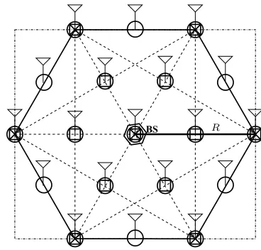
In the context of our investigation, four types of antenna dis-tribution patterns are considered, which are shown in Fig.1. Specifically, when the BS has only one antenna, certainly, this antenna is located at the BS. When the BS has 7 antennas, then, one of them is located at the BS, while the rest 6 are located at six corners of the hexagon, as indicated by the crosses (_×) in Fig.1. Similarly, when the BS employs 13 antennas, these 13 antennas are located at the positions indicated by the squares (¤) seen in Fig.1. Finally, when the BS employs 19 antennas, these 19 antennas are located at the positions indicated by the circles (_°) seen in Fig.1. We assume that the distributed anten-nas are connected with the BS at the cell center using optical

fibber and the signals received by the distributed antennas are directly sent to the BS without any processing at the distributed antenna locations. All signals are only processed at at the BS. Note that, in Fig.1,Ris the radius of the cell considered.

BS R

Fig. 1. A concept cell having one antenna at the base-station (BS), or 7, 13, 19 antennas distributed around the BS indicated by different shapes. Specifically, when the BS has 7 antennas, these antennas are distributed at the locations indicated by the cross (_×). When the BS has 13 antennas, these antennas are distributed at the locations indicated by the squares (¤). Finally, when the BS has 19 antennas, they are distributed at the locations indicated by the circles (°).

B. Channel Model

In this section the channel model for evaluating the perfor-mance of the distributed antenna MIMO systems is described. Let rk(t) be the received signal from a MS by thekth dis-tributed antenna. Upon neglecting the effect of thermal noise, the overall uplink received signal can be expressed as

r(t) =

N X

k=1

rk(t) (13)

re-ceived signal,rk(t), of thekth distributed antenna can be writ-ten as

rk(t) =αk(t)ρk(t){

√

P s(t)_}, k= 1, ..., N (14)

wheres(t)represents the signal transmitted by the MS, which

is normalized such thatE[_|s(t)_|2_{] = 1, while P denotes the} transmitted power. In (14)ρk(t) represents the envelope en-compassing the fast fading. By contrast, αk(t) accounts for large-scale geographical variation [9]. Upon absorbing the av-erage path loss intoαk(t),ρk(t)can be viewed as having unit mean-square value, i.e.,E[_|ρk(t)|2] = 1. Hence, the short-term power received by thekth antenna can be expressed as

ξk =|rk(t)|2=P · |αk(t)|2· |ρk(t)|2=lkP|ρk(t)|2 (15) wherelk = |αk(t)|2. Eq. (15) shows that the overall enve-lope of the power received by thekth distributed antenna has

a lognormal distribution, which is governed by the variable of

lk. Furthermore, it can be shown that, for independent lognor-mal distributed variablelk,10 log10lk has a Gaussian distribu-tion [10]. The practical measured data shows that the standard deviationσk in this Gaussian distribution ranges from 6 dB to

12 dB [9] and its mean equals to

µk=−βk·10 log10dk (16) wheredk =d/d0,ddenotes the distance between the MS and thekth distributed antenna, whiled0represents the close-in ref-erence distance, which is determined from measurements close to the transmitter. Furthermore, in (16)βk represents the as-sociated path loss exponent, which takes a value of 2 in a free space, and a value of 4 in cellular mobile communications sys-tems. Upon taking the above-mentioned issues into account, the PDF oflkcan be expressed as

flk(x) =

10

√

2πσlklk·ln 10

exp[₋(10 log10x−µk)

2

2σ2

k

] (17)

Letγk =ξkγcbe the short-term signal-to-noise ratio (SNR) contributed by thekth receive antenna, whereγc=P/N0 rep-resents the SNR in the corresponding AWGN channels. Then, when assuming that an optimum combiner is employed by the BS for combining the received signals from theN number of

distributed antennas, the total SNR achieved is given by

γ=γc× N X

k=1

γk (18)

The above equation is suitable for the distributed antenna as-sisted wireless systems, where a mobile user employs only one transmit antenna. When the mobile user employs multiple, say

U, transmit antennas, and when we assume that the space-time

coding achieving a full transmit diversity is employed, (18) then can be written as

γ=γc× U X

u=1 N X

k=1

γuk (19)

wherePU

u=1γukγcrepresents the SNR contributed by thekth receive antenna after the space-time decoding. Let us now con-sider the outage probability of the MIMO wireless systems us-ing distributed antennas.

C. Outage Probability

In a MIMO wireless system using distributed antennas, the SNRγreceived by the BS from a given mobile should exceed

a certain value, sayγT, in order to achieve a satisfactory recep-tion. Otherwise, an event of outage occurs. Hence, the outage probability can be expressed as

Pout = P(γ < γT)

= P

Ã

γc× U X

u=1 N X

k=1

γuk< γT !

(20)

Note that, in our simulation γT is set to be 4 dB.

IV. SIMULATIONRESULTS

In this section we provide a range of simulation results for the MIMO distributed antenna systems in the context of the average received power by the base station or of the outage probability. Note that, the total average received power illustrated in the

figures in this section represents its normalized quantity, which is given by

ξ=

n X

k=0

k¯¯ρk(t)¯¯ 2

(21)

Note furthermore that, in our simulation examples in the con-text of the received power, we assumed that the radius of the cell wasR = 6km, the path-loss exponent wasβk = 6dB. Four types of distributed antenna patterns were considered, which were shown in Fig.1 in correspondence withN = 1,7,13and

19 number of distributed antennas. Furthermore, we assumed that a mobile moved randomly in the rectangular areas (dash-dot line) as shown in Fig.1.

Figs.2 to 5 show the total received power versus mobile’s lo-cation performance of the conventional single antenna system and the wireless communications systems using various num-ber of distributed antennas. Specifically, in these figures the total received power by the BS was simulated, when the mobile moved at different locations in the squared area bordered by the dash-dot lines. The antenna distribution patterns were shown in Fig.1, in the context ofN = 1,7,13and 19. From the results

of Fig.2, it can be observed that the received power varies from about -25dB to 80dB, and the received power from the mobile in most case is low, when the mobile moves in the covered area by the cell. From the results of Fig.2 we can be implies that, unless the mobile is close to the BS at the center of the cell, it has to transmit a high power in order to achieve a relatively low outage probability.

−6 −4

−2 0

2 4

6

−6 −4 −2 0 2 4 6 −40 −20 0 20 40 60 80 100

x y

Power(dB)

Fig. 2. The total received power by the base station in a conventional wireless system using single receive antenna located at the center of the cell, when a mobile at different locations.

−6 −4

−2 0

2 4

6 −6 −4

−2 0

2 4

6 −20

0 20 40 60 80 100

y x

Power(dB)

Fig. 3. The total received power by the base station in a wireless system using 7 distributed antennas at locations shown by the crosses (×) in Fig.1, when a mobile at different locations.

areas showing the power peaks, the BS is capable of receiving a relatively high power. Specifically, Fig.3 shows 7 power peaks in correspondence with the wireless system using 7 distributed antennas. Fig.4 has 13 power peaks, since the cell uses 13 dis-tributed antennas. Finally, in Fig.5 there are 19 power peaks for the wireless system using 19 distributed antennas. From the re-sults of Figs.2 to 5 it can be shown that the BS has a higher and higher chance to receive a relatively high power, when increas-ing the number distributed antennas in a cell. This high chance of receiving higher power implies that a lower outage probabil-ity can be obtained, when a wireless communications system uses more distributed antennas, which can be shown below in Fig.6 and Fig.7.

Finally, in Fig.6 and Fig.7, we evaluated the outage versus SNR performance for the MIMO wireless communications

sys-−6 −4

−2 0

2 4

6 −6 −4

−2 0

2 4

6 −20

0 20 40 60 80 100

y x

Power(dB)

Fig. 4. The total received power by the base station in a wireless system using 13 distributed antennas at locations shown by the squares (_¤) in Fig.1, when a mobile at different locations.

−6 −4

−2 0

2 4

6 −6 −4

−2 0

2 4

6 −20

0 20 40 60 80 100

y x

Power(dB)

Fig. 5. The total received power by the base station in a wireless system using 19 distributed antennas at locations shown by the circles (_°) in Fig.1, when a mobile at different locations.

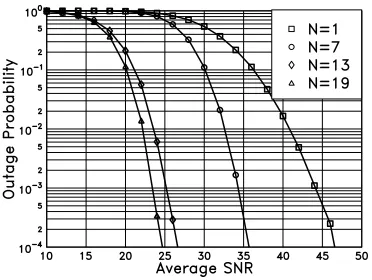
tems using distributed antennas. Specifically, in our simula-tions we assumed that, for both Fig.6 and Fig.7, the radius of the cell considered was R = 10km, and the cell employed

N = 1,7,13or 19 receive antennas distributed according to

Fig.1. Additionally, associated with Fig.6 we assumed that the mobile used only one transmit antenna, while with Fig.7 the mobile employed two transmit antennas and the transmit-ted data was space-time coded. In both Fig.6 and Fig.7 we as-sumed that the transmitted signal experienced lognormal shad-owed Rayleigh fading having a parameter ofσlk = 6dB and

Fig. 6. Outage probability of the distributed antenna wireless communica-tions system usingN = 1,7,13or 19 number of distributed antennas, when

the radius of the cell isR= 10km, the threshold isγT = 4dB, and when

communicating over a lognormal shadowed Rayleigh fading channel having the parameter ofσl_k= 6dB and a pathloss factor ofβk= 4dB.

Fig. 7. Outage probability of the space-time coding assisted distributed an-tenna wireless communications system usingN = 1,7,13or 19 number of

distributed antennas, when the radius of the cell isR= 10km, the threshold

isγT = 4dB, and when communicating over a lognormal shadowed Rayleigh

fading channel having the parameter ofσl_k = 6dB and a pathloss factor of

βk= 4dB.

the best outage performance among all the cases, while the con-ventional wireless system using no distributed antenna has the worst outage performance. As shown in Fig.6, at an outage probability of10−4_{, the required SNR is about 27dB for the} system using 19 number of distributed antennas, 29.5dB for the system using 13 number of distributed antennas, 39dB for the system using 7 distributed antennas, and,finally, 57dB for the system using one antenna. These results show that, when an existing wireless system employs 19 distributed antennas in-stead of only one at the BS, 30dB SNR gain might be achieved. We can also have the above observations from the results of Fig.7, where two transmit antennas were employed by the MS. Furthermore, upon comparing the results of Fig.7 with that of

Fig.6, it can be shown that, for a given number of distributed antennas, further SNR gains can be obtained owing to the mul-tiple transmit antennas and space-time coding employed by the MS.

V. CONCLUSION

In this contribution we have proposed and investigated a dis-tributed antenna MIMO wireless system, where multiple BS antennas are distributed in the area covered by a cell. Specif-ically, we have investigated the performance of the distributed antenna MIMO wireless system in the context of the total re-ceived power by the BS from a mobile station as well as of the outage probability, when the distributed antenna MIMO sys-tem without and with using space-time coding. Our simulation results in a lognormal shadowed Rayleigh fading environment show that, in a distributed antenna wireless system, both the number of antennas and the locations of antennas affect the sys-tem performance significantly. The performance of a wireless system can be significantly improved, by increasing the num-ber of distributed antennas and/or increasing the numnum-ber of mo-bile transmit antennas associated with using space-time coding. From our study in the context of the distributed antenna MIMO systems, we can expect that MIMO techniques will play an im-portant role in the future generations of mobile communications systems and standards, while MIMO techniques have already been incorporated into wireless LAN standards such as IEEE 802.11 and HiperLAN/2.

REFERENCES

[1] D.Gesbert, M.Shafi, Da-shan Shiu,P.J.Smith and A.Naguib,“From theory to practice:an overview of MIMO space-time coded wireless systems”,

IEEE J. Select. Areas. Commun., vol.21, NO.3, pp.281-302, April 2003 [2] A. Goldsmith, S. A. Jafar, N. Jindal, and S. Vishwanath, “Capacity limits

of MIMO channels,”IEEE Journal on Selected Areas in Communications, vol. 21, no. 5, pp. 684–702, June 2003.

[3] J.H.Winters, ”On the capacity of radio communication systems with di-versity in a Rayleigh fading environment”,IEEE J. Select. Areas Com-mun., vol.SAC-5, pp.871-878, June 1987.

[4] E.Telatar, “Capacity of multi-antenna Gaussian channels”ATT Bell Lab-oratories, Tech. Memo., June 1995.

[5] G.J.Foschini and M.J.Gans, “On limits of wireless communications in a fading environment when using antennas”,Wireless Pers. Commun., vol.6, pp.311-335, March 1998.

[6] Siavash M.Alamouti, “A simple transmit diversity technique for wire-less communications”,IEEE J. Select. Areas. Commun., vol.16, NO.8, pp.1451-58, Oct.1998.

[7] V.Tarokh, H.Jafarkhani and A.R.Calderbank, “Space-time block coding for wireless communications: performance results”,IEEE J. Select. Ar-eas. Commun., vol.17, NO.3, pp.451-60, March 1999.

[8] S. Verdu,Multiuser Detection. Cambridge University Press, 1998. [9] Q.T.Zhang, “Co-channel interference analysis for mobile radio suffering

lognormal shadowed Nakagami fading”,IEE Proc. Commun, vol. 146, NO.1, Feb.1999.

[10] T.S.Rappaport, Wireless Communication: Principles and Practice, Prentice-Hall, 1996.