Working Paper No. 286
March 2009
www.esri.ie
Mapping Patterns of Multiple Deprivation Using
Self-Organising Maps: An Application to EU-SILC Data for Ireland
Maurizio Pisati*, Christopher T. Whelan**, Mario Lucchini* and
Bertrand Maître***
Abstract: The development of conceptual frameworks for the analysis of social
exclusion has somewhat out-stripped related methodological developments. This paper seeks to contribute to this process through the application of self-organising maps
(SOMs) to the analysis of a detailed set of material deprivation indicators relating to the Irish case. The SOM approach allows us to offer a differentiated and interpretable picture of the structure of multiple deprivation in contemporary Ireland. Employing this approach, we identify 16 clusters characterised by distinct profiles across 42 deprivation indicators. Exploratory analyses demonstrate that position in the income distribution varies systematically by cluster membership. Moreover, in comparison with an analogous latent class approach, the SOM analysis offers considerable additional discriminatory power in relation to individuals’ experience of their economic circumstances. The results suggest that the SOM approach could prove a valuable addition to a ‘methodological platform’ for analysing the shape and form of social exclusion.
Corresponding Author: [email protected]
*University of Milano Bicocca, **University College Dublin, ***ESRI Dublin
Mapping Patterns of Multiple Deprivation Using
Self-Organising Maps: An Application to EU-SILC Data for Ireland
1. Introduction
The widespread adoption of the terminology of social exclusion/inclusion in Europe reflects inter alia an emerging consensus regarding the limitations of poverty research that focuses solely on income. Kakwani and Silber (2007, p. xv) identify the most important recent development in poverty research as the shift from a uni-dimensional to a multi-dimensional approach. Progress in this area can be viewed against the background of attempts to implement Townsend’s (1979) understanding of poverty as exclusion from ordinary living patterns, customs and activities because of resources that are substantially below average levels and Sen’s (2000) broader ‘capabilities’ and ‘functionings’ framework.
At the level of conceptualisation, the case for a multi-dimensional approach to understanding what it means to be socially excluded is compelling. However, as Nolan and Whelan (2007) argue, the value of such a perspective needs to be empirically established rather than being something that can be read off the multidimensional nature of the concept. Approaches that produce higher rather than lower dimensional profiles are not intrinsically superior. At this point, it seems to be generally agreed that many unresolved conceptual and measurement issues remain in the path of seriously implementing multidimensional measures in any truly operational sense (Thorbecke, 2007).
In this paper we seek to contribute to developing what Grusky and Weeden (2007, p. 33) describe as “a methodological platform” for analysing the shape and form of social exclusion. We do so specifically in relation to forms of material deprivation. A number of earlier efforts have employed latent class analysis to map patterns of material deprivation.1 The basic idea underlying such analysis is that the associations
1
between a set of categorical variables, regarded as indicators of an unobserved typology, are accounted for by membership of a small number of underlying classes. Latent class analysis assumes that each individual is a member of one and only one of C latent classes and that, conditional on latent class membership, the manifest
variables are mutually independent of each other. Where this assumption is justified, considerable gains can be achieved in terms of parsimony and understanding of underlying processes.
When the number of indicators of the latent typology of interest is large, several analytic difficulties arise from data sparseness, making it necessary to resort to a number of simplifying assumptions and procedures. One such approach consists in conducting latent class analysis in two stages, where dichotomised dimensions from the first stage are used as input at the second stage (Dewilde, 2004). An alternative approach has involved first conducting confirmatory factor analysis to identify a range of deprivation dimensions, and then entering categorical versions of the extracted factors into a latent class analysis (Whelan and Maitre, 2007). Such approaches have tended to start with the objective of moving fairly rapidly from highly detailed description of multiple outcomes to identification of a small number of underlying classes or clusters. An analytic strategy of this kind can clearly be justified in terms of the value of such simplifying assumptions in enabling us to identify underlying patterns relating to the detailed matrices constituted by large numbers of deprivation items and respondents. However, the question remains as to what extent these assumptions may influence our conclusions and, in particular, conceal important within-cluster heterogeneity.
synthetic measures or other forms of reduction of the complexity of input to the clustering procedure. The analytical tool for implementing this approach, self-organising maps (SOMs henceforth), is presented in the next paragraph.
2. Self-organising maps
Usually the groups into which researchers classify their observations are known in advance and correspond to the values taken on by particular variables or combination of variables. In some cases, however, the groups of interest are not known a priori and must then be discovered using suitable classification techniques. Self-organising maps is one such technique that combines the best properties of both classical clustering algorithms and projection methods, providing them with considerable potential value in analysing complex multi-dimensional data.
SOMs are an artificial neural network algorithm developed by Kohonen in the early 1980s to extract meaningful patterns from complex data and display them in an orderly fashion (Kohonen, 1982, 2001). Essentially, what the SOM algorithm does is to project a high-dimensional dataset X onto a lower dimensional output space so as to represent X in a compact form and easily identify its underlying structure. To clarify how this projection works and the outcomes it generates, we proceed as follows: first, we define the basic ingredients of any SOM, i.e., the input data X and the corresponding output space; then, we offer a basic description of the SOM algorithm.
The starting point of a standard SOM analysis is a case-by-variable dataset, formally defined as a matrix X whose rows represent observations and whose columns represent their attributes of interest. The d elements that make up each row i of X
( ) correspond to the values taken by each attribute j ( ) on
d
n×
n
observation i; together, they are referred to as the input vector and represent the coordinates of observation i in the d-dimensional input space .
i
x
m d
ℜ
,...,
A SOM can be seen as an analytical procedure that helps to reduce the complexity of
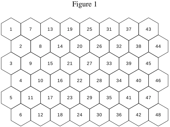
X by projecting it onto a lower dimensional output space. This space corresponds to the SOM itself and, typically, takes the form of a two-dimensional grid,2 i.e., a rectangular array of m cells arranged in a square or hexagonal lattice (see Figure 1 for an illustration). Each grid cell is called a unit, or node, and can be regarded as a pole specialized in attracting observations that possess certain combinations of attributes; projecting X onto the SOM, then, amounts to allocating each observation i to the unit that attracts it most. More precisely, each SOM unit k (k ) is characterised by a unique weight vector that belongs to the same coordinate space as the input vectors – i.e., ; this means that the input vectors can be systematically compared with the weight vectors and each observation i can be properly allocated to its best matching unit – i.e., to the SOM unit whose weight vector is closest (most similar) to the input vector . Formally, we say that the SOM partitions the input space into m Voronoi regions, each of which corresponds to a specific SOM unit k and attracts all the input vectors that are closer to its generating point than to any other generating point. If properly realized, this partition is such that the Voronoi regions that are close in the input space are also close in the output space, i.e., their corresponding SOM units are spatially contiguous on the two-dimensional grid. This property is called topology preservation and is one of the most appealing features of SOMs, since it makes for a clearer and more accurate representation of the structure of the input data.
1 =
d
×
1 wk
k∈ℜ i
x w d
d
i
x
ℜ
k
w
[FIGURE 1 ABOUT HERE]
2
To sum up, projecting a d-dimensional dataset X onto a two-dimensional SOM amounts to (a) computing the weight vectors associated with the m SOM units; and (b) on the basis of these weights, allocating each observation i to its best matching unit. To achieve this result, the SOM goes through a competitive learning process – also known as training process – that incrementally adjusts the weight vectors according to a set of rules aimed at maximizing both the discriminatory power of the map (i.e., the map resolution) and its degree of topology preservation. The learning process begins by assigning proper starting values to each weight vector and develops over T iterations called learning epochs. For every learning epoch t, each input vector , in turn, is “learnt” by the SOM; therefore, the whole learning process is made of learning steps. At each learning step , weight vectors are adjusted as follows:
k w k w i x
L=n×T
3
Compute the distance between the input vector and each weight vector . ik D ik D i x ) 1 ( − k
w 4 Typically, is the Euclidean distance xi −wk( −1) .
Identify the best matching unit of – i.e., the SOM unit corresponding to the minimum value of – and denote it by index b.
i
x
ik D
Adjust the weight vector of each SOM unit k as follows: )] 1 ( )[ ( ) ( ) 1 ( )
( = k − + kb i− k −
k w t t x w
w α ν
This formula shows that the weight vector at learning step is equal to the weight vector at learning step plus an adjustment factor
k w − k w ( − 1 )] 1 )[ ( )
(tνkb t xi−wk
α . Here, the term [ indicates that the adjustment
of the weight vector adds up to making it incrementally closer to the input vector under consideration – and, therefore, to making the corresponding SOM unit incrementally more ‘attractive’ for that input vector. The extent to which this ‘approaching’ takes place depends on the value taken on by the neighbourhood kernel
)] 1 −
i
x −wk(
k
) (t kb
w
ν , which is a decreasing function of the spatial distance between each unit k and
3
For more details on the SOM algorithm, its practical implementation and its variants, see Oja and Kaski (1999), Allinson et al. (2001), Kohonen (2001), Obermayer and Sejnowski (2001), Samarasinghe (2007).
4
the best matching unit b on the two-dimensional grid. In general, this means that the closer a given SOM unit k is to the best matching unit b, the greater is the degree to which its weight vector is adjusted toward the input vector ; for example, if unit 22 in Figure 1 is the best matching unit, then the adjustment will be maximum for unit 22 itself, somewhat smaller for the units in its immediate surroundings (16, 21, 27, 28, 29, 23), even smaller for its second-order neighbouring units (15, 14, 20, 26, 33, …), and so on.
k
w xi
5
The value of the neighbourhood kernel is regulated the neighbourhood radius σ(t) parameter, which defines the width of the kernel itself and is a strictly decreasing function of t.6 Finally, the overall degree of weight vector adjustment is controlled by the learning rate parameter – denoted by α(t); this parameter is a multiplier in the interval that regulates the velocity of weight vector adjustment and is a strictly decreasing function of t.
] 1 , 0 [
7
When the training is concluded, each observation i can be allocated to its final best matching unit, i.e., to the SOM unit that minimizes the distance between and
. The end result of this allocation is the classification of the n observations of interest into
ik
D xi
) (L k
w
m
g≤ exhaustive and mutually exclusive groups.8
SOMs have found wide application in such diverse fields as image analysis, speech recognition, engineering, chemistry, physics, mathematics, linguistics, medicine, biology, ecology, geography, marketing and finance (Kaski et al., 1998; Oja et al., 2003), but much less so in sociology. Recently, attempts have been made to extend SOM analysis to the study of multiple deprivation in Italy (Lucchini and Sarti, 2005;
5
It is true that this example applies only when the neighbourhood kernel is a strictly decreasing function of the distance between units k and b.
6
This implies that, when setting up the SOM, it is necessary to specify the initial value of the neighbourhood radiusσ(1), the final value of the neighbourhood radius σ(T), and the radius decay function.
7
As with the neighbourhood radius, the dependence of α(t) on t requires that, when setting up the SOM, the initial value of the learning rateα(1), the final value of the learning rate α(T), and the rate decay function be specified.
8
Lucchini et al., 2007). In this paper we take advantage of the availability of detailed data relating to material deprivation for a large representative sample in the Irish component of the European Union Community Statistics on Income and Living Conditions (EU-SILC) instrument to extend such efforts.
3. Overview of the analysis
Below we describe the data on which our analysis is based and the key variables. We then provide an account of the technical details relating to the application of SOM procedures to the Irish data, including weighting of vectors and choice of ‘training’ parameters. We proceed to analyse the configuration of the trained SOM by examining some representative examples of a type of specialized graphs known as component planes. Focusing on a number of key indicators, we illustrate the
discriminatory power of the SOM by distinguishing three groups of nodes in the two-dimensional grid, characterised in terms of their relative ‘specialisation’ in attracting disadvantaged, average and advantaged individuals. We go on to partition the output space of the SOM units into a smaller set of homogeneous regions which we consider to offer a reasonable balance between detail and parsimony and map this outcome. To aid in the interpretation of this clustering outcome, we employ a multidimensional scaling algorithm to project the clusters onto a two-dimensional space illustrating their relative size and location.
Finally, we provide an exploratory analysis of the validity of the SOM typology. We do so initially by showing the extent to which cluster membership is differentiated in terms of household income. We proceed to compare the clustering outcome deriving from SOM analysis to that resulting from the application of latent class procedures to the same set of indicators. Lastly, we provide an assessment of the extent to which the clusters identified utilising the SOM procedure offer additional discriminatory capacity in relation to the manner in which economic circumstances are experienced.
4. Data and variables
The data used in this paper are drawn from the 2004 wave of the Irish EU-SILC survey, a voluntary annual survey of private households conducted by the Central Statistics Office (CSO). In 2004, the total completed sample size was 5,477 households and 14,272 individuals, with a declared response rate equal to 48% (CSO, 2005). The analysis reported here refers to all persons in the EU-SILC. Where household characteristics are involved, these have been allocated to each individual. The HRP is the one responsible for the household accommodation and their characteristics have been attributed to all individuals in the household.
Our analysis makes use of forty-two dichotomous indicators of deprivation.9 A confirmatory factor analysis of these forty-two items by Maître et al. (2006) revealed the following relatively distinct deprivation dimensions:
1. Basic deprivation: eleven items relating to food, clothing, furniture, debt, and minimal participation in social life.
2. Consumption deprivation: nineteen items.
9
3. Household facilities deprivation: four items regarding basic facilities such as bath, toilet etc.
4. Neighbourhood environment deprivation: five items concerning pollution, crime/vandalism, noise, and deteriorating housing conditions.
5. Health deprivation: three items relating to overall evaluation of health status of the HRP, having a chronic illness or disability and restricted mobility.
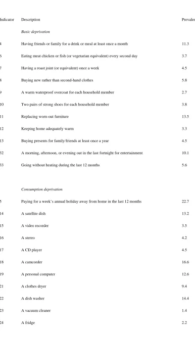
Details of the indicators comprising each of the dimensions are set out in Table 1
[TABLE 1 ABOUT HERE]
5. Results
5.1. SOM training and interpretation
The starting point of our analysis10 is a 14,219×42 matrix11 which we project onto a two-dimensional SOM made of 432 units arranged in a 18×24 hexagonal lattice12. Weight vectors were initialised using the linear method (Kohonen, 2001), and the SOM training was carried out in two phases:
1. An 8-epoch ordering phase, based on a large initial value and a fast decrease of both the neighbourhood radius (σ(1)=20,σ(8)=10, linear decay function) and the learning rate (α(1)=1,α(8)=0.1, linear decay function).
10
All the analyses reported in this paper, including SOM training and visualization, have been carried out using routines written in the Stata programming language (StataCorp, 2007).
11
53 observations have been eliminated from the analysis because they were missing on one or more of the forty-two indicators.
12
2. A 50-epoch fine-tuning phase, based on a minute and slow adjustment of both the neighbourhood radius (σ(1)=10,σ(50)=1, linear decay function) and the learning rate (α(1)=0.1,α(50)=0, linear decay function).13
At the end of the training process, each observation was allocated to its final best matching unit and the quality of the SOM was assessed by means of two measures: the quantization error and the topographic error (Kohonen, 2001). The quantization error – normalized so as to take values in the interval – is a measure of the SOM resolution and corresponds to the average distance between each input vector and its best matching unit; our SOM exhibits a normalized quantization error equal to 0.124, meaning that – on average – each element of the input vector differs from its corresponding best-matching-unit weight by 12.4 percentage points. In turn, the topographic error is a measure of the SOM’s degree of topology preservation and
corresponds to the proportion of all input vectors for which the best matching unit and the second-best matching unit are not adjacent on the two-dimensional grid; our SOM exhibits a topographic error equal to 0.009, meaning that only 128 observations are affected by some degree of ‘topological misplacement’.
] 1 , 0 [
i
x
To analyse the configuration of the trained SOM, we visually inspect its component planes, a kind of specialized graph that illustrates the value taken by a given element
of the weight vector on each SOM unit. Some representative component planes, each corresponding to a distinct element of – and, therefore, to a specific indicator of deprivation – are shown in Figure 2. As we can see, in each graph SOM units are classified into up to three distinct groups: (a) black units ‘specialise’ in attracting ‘disadvantaged respondents’, i.e., observations that take value 1 on the corresponding indicator; (b) grey units ‘specialise’ in attracting ‘advantaged respondents’, i.e., observations that take value 0 on the corresponding indicator; (c) white units have no clear-cut ‘specialisation’, i.e., attract a more or less balanced mix of observations of
k
w
k
w
13
both types.14 The spatial distribution of these three types of units on the two-dimensional grid describes the configuration of the SOM in terms of the corresponding indicator.15
In order to clarify what is involved, we first consider the component plane representing ‘inability to afford a video recorder’ (Figure 2, panel a). As we can see, in this case the vast majority of SOM units belong to the ‘neutral’ (white) category, i.e., attract a quota of disadvantaged respondents that is not substantially different from that observed in the working dataset (4%, see Table 1). There is also a small cluster of ‘hot’ (black) units, i.e., units that attract a disproportionate share of disadvantaged. In contrast, there are no ‘cold’ (grey) units, i.e., units that attract a number of disadvantaged respondents substantially lower than the average.16 It is worth noting that a similar pattern holds for the inability to afford a range of other durables, including a vacuum cleaner, a fridge, a freezer, a micro wave, a deep fat fryer, a liquidiser, a video, a stereo, and a washing machine. For this set of items, therefore, we observe a weak pattern of discrimination combined with a sharp pattern of spatial differentiation between the small number of ‘hot’ units and all the others.
[FIGURE 2 ABOUT HERE]
For more expensive consumer durables, a more typical pattern is that represented by the component plane shown in Figure 2, panel b (inability to afford a personal computer). A tripartite division emerges with half or more of the SOM units being neutral. Of the remaining units, the grey ones are slightly more frequent than the black ones. While the latter tend to be clustered in the upper left-hand corner of the SOM,
14
It is important to note that ‘specialisation’ here, should be understood in relative terms.
15
Typically, component planes represent the distribution of SOM weights in more detail, i.e., by means of a larger number of ordered classes. For illustrative purposes, however, the threefold repartition described above has the merit of conveying a sufficient amount of information in a compact way.
16
the remaining units are more widely distributed. This pattern also applies to the inability to afford a clothes dryer, a dish washer, and a satellite dish. Moreover, a similar pattern is observed for the inability to afford a car, a camcorder, and new furniture; in these cases, however, the number of neutral units is a good deal lower.
For all the indicators of health deprivation, the component plane is close to that shown in Figure 2, panel c, with a significant majority of cold units, a significant minority of hot units, and a much smaller minority of neutral units. The item regarding the inability to afford a holiday exhibits a similar pattern. Thus, for these items we observe a pattern of differentiation which involves a very modest intermediate ground.
As regards the absence of basic household facilities, both hot and cold units are more widely dispersed in the two-dimensional space. This is illustrated in Figure 2, panel d, for the item indicating rooms being too dark or without light. In this case we have a very substantial quota of neutral units from whom the remaining units are distinguished in a bipolar fashion.
Finally, the neighbourhood environmental items are distinguished by the fact that hot units form two spatially separate clusters, suggesting that multiple and distinct influences may underlie this form of deprivation. The component plane representing crime, violence or vandalism in the area of residence typifies this pattern (see Figure 2, panel e).
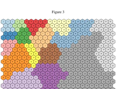
5.2. Clustering the SOM units
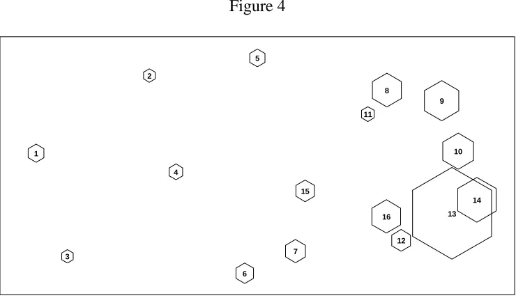
As illustrated in the previous section, the visual inspection of the forty-two component planes associated with our SOM reveals the fine structure of the underlying input space. Treating each SOM unit individually would require dealing with an overwhelming level of detail. To address this issue, we partition the output space (i.e., the 432 SOM units) into a smaller set of sufficiently homogeneous regions (i.e., clusters of SOM units), using weight vectors as the clustering variables (Vesanto and Alhoniemi, 2000; Wu and Chow, 2004) and the hierarchical agglomerative average linkage method as the clustering algorithm (Kaufman and Rousseeuw 1990). Based on careful inspection of the component planes, experimentation and past experience (Lucchini et al., 2007), we opt for a 16-cluster solution that offers a reasonable balance between detail and parsimony. Figure 3 displays the result of this operation. It is worth noting that, without imposing any constraint to the clustering algorithm, each cluster turns out to be entirely made of spatially contiguous SOM units.
[FIGURE 3 ABOUT HERE]
To aid interpretation, we project the sixteen clusters of SOM units onto a two-dimensional space so as to maximize the correlation between the location of the clusters in the data space and the location of the clusters in the plane; to this aim, we use a classical metric multidimensional scaling algorithm (Torgerson, 1952) adjusted ex post via a genetic algorithm (Mitchell, 1996). The result of this projection is shown
size and location, offering a differentiated picture of the structure of multiple deprivation in contemporary Ireland.
[FIGURE 4 ABOUT HERE]
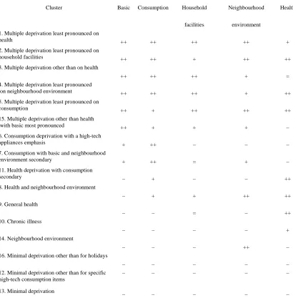
A detailed description of the resulting structure is provided in Figure A1, where we display the prevalence of the forty-two indicators of deprivation within each of the sixteen clusters. In order to provide a summary of this large mass of information, we develop the profile for each cluster relating to deviations around the mean levels of the five dimensions as described earlier, comprising basic, consumption, household facilities, neighbourhood environment, and health.
In developing these profiles, we have pursued a strategy seeking to synthesize the information given by each single indicator in a way that takes into account the strongly skewed distribution of almost all the indicators. Namely:
1. For each indicator Xj ( 1,…,42), we have computed its sample variance )
1
( , where Xj =1). = j Pr( = j p )
(Xj pj pj
V = −
2. For each indicator Xj, we have computed two threshold values: 75 . 0 ) ( ln
1 ⎟⎟
⎠ ⎞ ⎜ ⎜ ⎝ ⎛ + × = j j j j p X V p t 5 . 1 ) ( ln
2 ⎟⎟
⎠ ⎞ ⎜ ⎜ ⎝ ⎛ + × = j j j j p X V p t .
3. For each indicator Xj, we have computed its mean within each cluster Cg (g=1,…,16):pj|g =Pr(Xj =1|Cg).
5. We have transformed the deviation values δjg into a corresponding set of discrete scores sjg according to the following rules:
⎪ ⎪ ⎩ ⎪ ⎪ ⎨ ⎧ > ≤ < ≤ ≤ − − < − = j jg j jg j j jg j j jg jg t t t t t t s 2 2 1 1 1 1 if 2 if 1 if 0 if 1 δ δ δ δ .
6. For each cluster Cg and each deprivation dimension Dq ( =1,…,5), we have computed the mean of the scores sjg pertaining to the relevant indicators:
q
∑
∑
= ∈ ∈ = d j q D j jg gq D j s q 1 ) ( μ .7. Finally, we have transformed the mean values μgq into a corresponding set of symbols according to the following rules:
" "
0 → −
< gq μ " "
0 → =
= gq μ " " 1
0<μgq ≤ → + " "
1 → ++
>
gq
μ .
The end result of this procedure is shown in Table 2.
[TABLE 2 ABOUT HERE]
Cluster 1 (Multiple deprivation least pronounced on health) is characterised by a fairly uniform pattern of deprivation which is least severe in relation to health. It comprises 1.8 per cent of the sample.
Cluster 2 (Multiple deprivation least pronounced on household facilities) also involves a relatively uniform pattern of deprivation that is more pronounced than for cluster 1 in relation to health but somewhat less so with regard to household facilities. It makes up 1.1 per cent of the sample.
Cluster 3 (Multiple deprivation other than on health) is characterised by above average deprivation in relation to all dimensions other than health but with the scale being somewhat weaker for neighbourhood environment than for the remaining dimensions. This group comprises 1.1 per cent of the population.
Cluster 4 (Multiple deprivation least pronounced on neighbourhood environment) is distinctive primarily in relation to health, basic, consumption and household facilities. It involves 1 per cent of the sample.
Cluster 5 (Multiple deprivation least pronounced on consumption) is distinguished from the foregoing clusters by a lower level of consumption deprivation. It makes up 1.7 per cent of the sample.
Cluster 15 (Multiple deprivation other than health with basic most pronounced) is made up of individuals displaying above average deprivation on all dimensions other than health, especially in relation to the dimension of basic deprivation. In terms of consumption, enforced absence of a car is particularly prevalent. It involves 2.3 per cent of the sample.
Cluster 6 (Consumption deprivation with a high-tech appliances emphasis) is characterised by basic and, above all, consumption deprivation, the latter particularly pronounced in relation to high-tech consumer durables and holidays. It comprises 2.4 per cent of the sample.
play less of a role. Neighbourhood environment joins basic deprivation as a secondary element. It involves 2.7 per cent of the sample.
Cluster 11 (Health deprivation with consumption secondary) it involves a combination of health and consumption deprivation. It is somewhat smaller than the two previous clusters, making up 1.1 per cent of the sample.
Cluster 8 (Health and neighbourhood environment) exhibits a profile of deprivation in relation to health and neighbourhood environment with consumption and household facilities playing a secondary role. It is the largest group up this point, involving 5.3 per cent of the sample.
Cluster 9 (General health) is distinguished from the other groups almost exclusively in terms of deprivation in relation to health. It comprises 7.8 per cent of the sample. Cluster 10 (Chronic illness) is also characterised almost entirely by deprivation in relation to health. In this case differentiation is less sharp and is largely in relation to chronic illness. It includes 6.2 per cent of the sample.
Cluster 14 (Neighbourhood environment) involves a pattern of minimal deprivation, with the crucial exception being in relation to neighbourhood environment. It is a relatively large group making up 10.7 per cent of the sample.
Cluster 16 (Minimal deprivation other than for holidays) is also characterised by a pattern of minimal deprivation other than with regard to enforced absence of a holiday. It includes 5.9 per cent of the sample.
Cluster 12 (Minimal deprivation other than for specific high-tech consumption items) is distinguished from cluster 13 almost entirely by deprivation in relation to high-tech items and, most particularly, in relation to a CD player and a satellite dish. It involves 2.7 per cent of the sample.
Cluster 13 (Minimal deprivation) displays a uniformly low pattern of deprivation. It is the largest group by far, comprising 46.2 per cent of the sample.
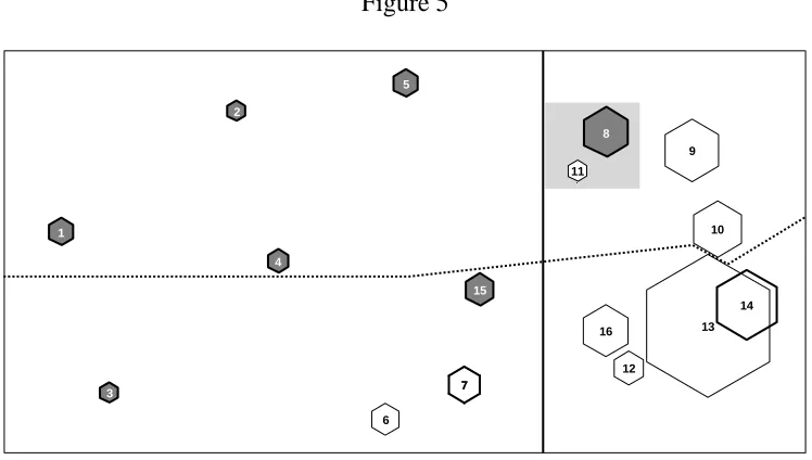
the line) from the ‘healthy’ clusters (below the line). In turn, the solid (vertical) line separates the clusters exhibiting a significant level of basic deprivation (left) from those that do not experience this form of deprivation (right). The area of consumption deprivation coincides with that of basic deprivation, with the addition of the small grey region comprising clusters 8 and 11. Dark grey clusters are also characterised by a substantial degree of deprivation in terms of household facilities. Finally, clusters with a thick black outline exhibit a relatively high degree of deprivation also in terms of neighbourhood environment.
[FIGURE 5 ABOUT HERE]
5.3. Validating the SOM clusters
We have identified a set of clusters that can be interpreted in meaningful substantive terms. Our results fulfil the criterion of face validity. Clearly, the next step is to undertake a systematic analysis relating to the construct validity of the typology of deprivation that we have identified. Such an analysis would require a range of multivariate analysis that cannot be accommodated within the constraints of the current paper. Instead what we provide is a simpler illustrative analysis relating to the manner to which the clusters are differentiated in socio-economic differentiation, the relationship between the SOM typology and the outcome of a latent class analysis of the same data, and the extent to which the former offers additional discriminatory capacity in relation to outcomes such as subjective economic stress.
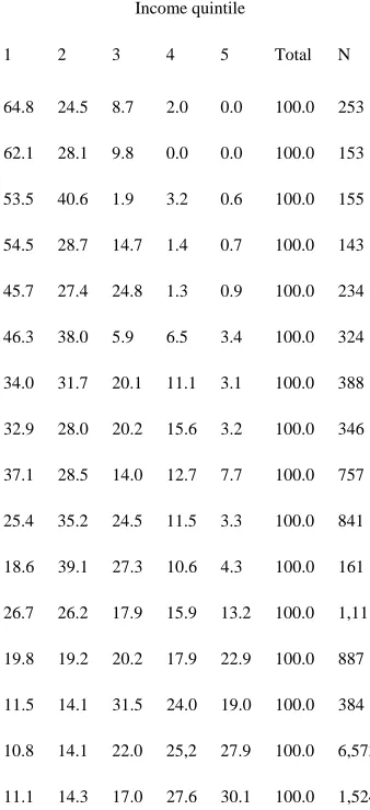
the two bottom quintiles into account this figure rises to 90 per cent. Correspondingly, the respective figures for the top two quintiles are respectively 2 per cent and zero.
The pattern of differentiation is only marginally less striking for clusters 3 and 4, representing respectively patterns of deprivation where consumption and consumption and health are the dominant elements. The number in the bottom quintile falls to the mid-50s with relatively proportionate increases across the remaining quintiles. For cluster 5, involving a pattern of health and basic deprivation, and cluster 15 involving the latter combined with enforced deprivation of a car, the figure in the bottom quintile falls to the mid-40s. In none of the six cases we have considered so far does the figure in the two bottom quintiles fall much below three-quarters and in no case does the number found in the top two quintiles rise above 2 per cent.
The foregoing categories can be clearly distinguished from clusters 6, 7 and 11 in terms of their tendency to be concentrated at the lower end of the income distribution. For these groups the number in the bottom quintile ranges between 33 and 37 per cent, and the corresponding figures for the top two quintiles run from 14 to 20 per cent.
[TABLE 3 ABOUT HERE]
When we turn to the clusters involving minimal deprivation, a further pronounced shift is observed. Cluster 14 is characterised by a uniform distribution of its members across the five quintiles (18-23 per cent of respondents in each quintile). In turn, clusters 16, 12 and 13 are characterised by a low probability of being located in the bottom quintile, with approximately 11 per cent being found there in each case. The total in the bottom two quintiles is uniform across the three clusters, with 25 per cent being so located. A divergence is observed in the numbers in the third quintile, with members of cluster 16 being a good deal more likely to be found there. The relevant figure declines from 32 per cent for cluster 16, involving deprivation on certain high tech consumer items, to 22 and 17 per cent respectively for clusters 12 and 13. Corresponding differences are observed in the number in the top quintile. This rises to from 19 per cent for cluster 16 to approximately 30 per cent for the other two clusters.
In the hierarchy of income differentiation, the next position is occupied by clusters 6, 7 and 11 which are characterised by relatively specific forms of consumption deprivation. Cluster 8, which is characterised by health deprivation accompanied by significantly more modest neighbourhood environment deprivation, displays a similar profile. The previous three clusters differ from the remaining health clusters 9 and 10, which are associated with substantially less skewed distribution of income.
In turn, the consumption and health clusters are clearly differentiated from the four remaining clusters involving minimal deprivation. The fact that the cluster involving solely neighbourhood environment (cluster 14) forms part of the group is likely to be a consequence of the fact that relatively affluent individuals may choose to endure such deprivation in return for the compensatory advantages conferred by particular urban locations.
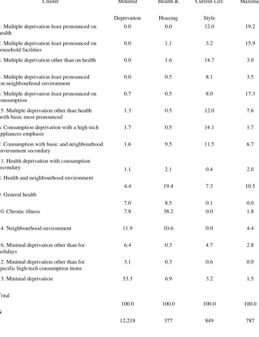
The set of deprivation indicators on which we have focused have been previously subjected to latent class analysis by Whelan and Maître (2007). They found that the best fitting solution involved four latent classes which they labeled as follows:
1. Minimally Deprived comprising 82.6 per cent of the sample.
2. Health and Housing Deprived making up 4.5 per cent of the sample.
3. Deprived in terms of current living standards (CLSD) involving 6.2 per cent of the sample.
4. Maximally Deprived incorporating 6.8 per cent of the sample.
latent class minimal deprivation group involves the allocation of 3 per cent of its membership to SOM consumption clusters 6 and 7, and 20 per cent to the health clusters 8-11.
[TABLE 4 ABOUT HERE]
Focusing on the latent class health and housing cluster, we find that over 90 per cent of this group have been allocated to SOM categories that have strong elements of deprivation relating to health, housing and neighbourhood environment. Focusing on the latent class CLSD cluster, we find that almost 50 per cent are found in the SOM consumption clusters 6 and 7 and in the multiply deprived clusters 3 and 4 which involve significant consumption elements. A further 35 per cent are found in the remaining multiply deprived clusters 1, 2, 5, and 15.
Finally, focusing on the latent class maximal deprivation cluster, we find that two thirds of its members are located in the SOM multiple deprivation clusters 1-5 and 15. A further 10 per cent are found in the clusters 6, 7 and 1, which involve significant consumption elements, while 11 per cent are located in cluster 8 characterised by health and neighbourhood environment deprivation. Contrary to expectation, about 9 per cent are found in the minimal deprivation and neighbourhood environment SOM clusters.
estimates. Even so we have had to exclude clusters 1 to 5 of the SOM typology. The economic stress indicator is derived from a question answered by the Household Reference Person relating to the extent to which, in comparison with other households, the household has ‘difficulty in making ends meet’. The dichotomous dependent variable on which we focus contrasts those individuals in households reporting “great difficulty” or “difficulty” with all others. From Table 5 we can see that, within the latent class minimal deprivation cluster, considerable variation in level of subjective economic stress is observed conditional on SOM cluster membership.
[TABLE 5 ABOUT HERE]
The lowest level of subjective economic stress of 11 per cent is observed for the SOM minimal deprivation cluster 13. A modest rise to 14 per cent is observed for neighbourhood environment (cluster 14) and general health (cluster 9). A further increase to approximately 20 per cent occurs for deprivation solely in relation to specific high-tech consumer durables and the chronic illness cluster. The figure increases to 33 and 37 for the remaining health groups, where consumption and neighbourhood environment respectively are accompanying aspects. For the consumption categories we observe a rise to 40 per cent where the secondary aspect relates to neighbourhood environment, and to 49 per cent for the broader consumption deprivation dimension incorporating high-tech consumer durables. The holiday cluster (cluster 16) occupies an intermediate position (44 per cent). Finally, cluster 15, which is characterised by basic deprivation and the enforced absence of a car, is quite distinctive and is associated with a level of economic stress of 85 per cent.
key factor, to those where health combines with other forms of deprivation, to more purely health clusters, and finally to clusters characterised by minimal deprivation. Taken together with the evidence on income differentiation, it provides strong support for the validity of the SOM typology in terms of its capacity to identify meaningful forms of multiple deprivation that can be accounted for by key socio-economic variables and have a significant influence on the manner in which individuals experience their economic circumstances. A more comprehensive demonstration that is the case will require undertaking an appropriate set of multivariate analyses.
6. Conclusion
The development of conceptual frameworks for the analysis of social exclusion and the pervasive use of related terminology in both academic and policy debates has somewhat out-stripped related methodological developments. This paper constitutes an effort to contribute to “a methodological platform” for analysing the shape and form of social exclusion (Grusky and Weeden, 2007, p. 31).
are contrasted with the rest in terms of basic deprivation, while these clusters, together with clusters 6 and 7, are also distinctive in terms of their levels of consumption. Cluster 8 and 11 occupy an intermediate position with regard to consumption. High levels of health deprivation distinguish clusters 1, 2, 4, 5 and 8 to 11. On the other hand, clusters 7 and 14 are distinctive in terms of neighbourhood environment.
Taken together, cluster 1 to 5 and 15 capture 9 per cent of the population who experience forms of multiple deprivation with varying emphasis on basic deprivation, health and neighbourhood environment. Clusters 6 and 7, comprising 5 per cent of the sample, are characterised by different forms of consumption deprivation with the distinction between high and low tech consumer durables playing an important role. Clusters 8 to 11, which are primarily differentiated in terms of health, make up 18 per cent of the sample. Clusters 9 and 10 are distinguished pretty well entirely by the health indicators while 8 and 11 combine significant elements of consumption and, in the case of cluster 8, neighbourhood deprivation. Clusters 14 and 16, involving respectively 11 and 6 per cent of the sample, are located towards the minimum deprivation end of the continuum and are distinguished, in turn, solely by deprivation relating to neighbourhood environment and inability to afford a holiday. Finally, clusters 12 and 13 represent relatively uniform patterns of minimal deprivation and comprise just less than one half of the sample.
Appendix
Figure A1
References
Allinson, N., Yin, H., Allinson, L., Slack, J. (Eds.), 2001. Advances in Self-Organising Maps. Springer, Berlin.
Central Statistics Office, 2005. EU Survey on Income and Living Conditions (EU-SILC); First Results 2003, Statistical Release 24 January, SO: Dublin/Cork.
Dewilde, C., 2004. The multidimensional measurement of poverty in Belgium and Britain: A categorical approach. Social Indicators Research 68, 331-369.
Dewilde, C., 2008. Multidimensional poverty in Europe: Institutional and individual determinants. Social Indicators Research 83, 233-256.
Grusky, D.B., Weeden, K.A., 2007. Measuring poverty: The case for a sociological approach. In: Kakwani, N., Silber, J. (Eds.), The Many Dimensions of Poverty. Palgrave Macmillan, Basingstoke, pp. 20-35.
Kakwani, N., Silber, J., 2007. Introduction. In: Kakwani, N., Silber, J. (Eds.), The Many Dimensions of Poverty. Palgrave Macmillan, Basingstoke.
Kaski, S., Kangas, J., Kohonen, T., 1998. Bibliography of self-organizing map (SOM) papers: 1981-1997. Neural Computing Surveys 1, 102-350.
Kohonen, T., 1982. Self-organized formation of topologically correct feature maps. Biological Cybernetics 43, 59-69.
Kohonen, T., 2001. Self-Organizing Maps, third ed. Springer, Berlin.
Lucchini, M., Sarti, S., 2005. Il benessere e la deprivazione delle famiglie italiane: un approccio multidimensionale e multilivello. Stato e mercato 74, 231-265.
Lucchini, M., Pisati, M., Schizzerotto, A., 2007. Stati di deprivazione e di benessere nell’Italia contemporanea: Un’analisi multidimensionale. In: Brandolini, A.,
Saraceno, C. (Eds.), Povertà e benessere: Una geografia delle disuguaglianze in Italia. il Mulino, Bologna, pp. 271-303.
Maître, B., Nolan, B., Whelan, C.T., 2006. Reconfiguring the Measurement of Deprivation and Poverty in Ireland. Economic and Social Research Institute, Policy Research Series, No. 58, Dublin.
Mitchell, M., 1996. An Introduction to Genetic Algorithms. The MIT Press, Cambridge, MA.
Moisio, P., 2004. A latent class application to the multidimensional measurement of poverty, Quantity and Quality 38, 703-717.
Obermayer, K., Sejnowski, T.J. (Eds.), 2001. Self-Organizing Map Formation: Foundations of Neural Computation. The MIT Press, Cambridge, MA.
Oja, E., Kaski, S. (Eds.), 1999. Kohonen Maps. Elsevier, Amsterdam.
Oja, M., Kaski, S., Kohonen, T., 2003. Bibliography of self-organizing map (SOM) papers: 1998-2001 addendum. Neural Computing Surveys 3, 1-156.
Samarasinghe, S., 2007. Neural Networks for Applied Sciences and Engineering: From Fundamentals to Complex Pattern Recognition. Auerbach Publications, Boca Raton, FL.
Sen, A., 2000. Social Exclusion: Concept, Application and Scrutiny. Social
Development Papers No. 1, Office of Environment and Social Development, Asian Development Bank, Manila.
StataCorp, 2007. Stata Statistical Software: Release 10. StataCorp LP, College Station, TX.
Thorbecke, E., 2007. Multidimensional poverty: Conceptual and measurement issues. In: Kakwani, N., Silber, J. (Eds.), The Many Dimensions of Poverty. Palgrave
Macmillan, Basingstoke, pp. 3-19.
Torgerson, W.S., 1952. Multidimensional scaling: I. Theory and method. Psychometrika 17, 401-419.
Vesanto, J., Alhoniemi, E., 2000. Clustering of the self-organizing map. IEEE Transactions on Neural Networks 11, 586-600.
Whelan, C.T., Maître, B., 2005. Economic vulnerability, multi-dimensional
deprivation and social cohesion in an enlarged European Union. International Journal of Comparative Sociology 46, 215-239.
Whelan, C.T., Maître, B., 2007. Levels and patterns of multiple deprivation in Ireland: After the Celtic Tiger. European Sociological Review 23, 139-156.
Table 1
Indicators of deprivation used in the analysis (N = 14,219)
Indicator Description Prevalence (%)
Basic deprivation
4 Having friends or family for a drink or meal at least once a month 11.3
6 Eating meat chicken or fish (or vegetarian equivalent) every second day 3.7
7 Having a roast joint (or equivalent) once a week 4.5
8 Buying new rather than second-hand clothes 5.8
9 A warm waterproof overcoat for each household member 2.7
10 Two pairs of strong shoes for each household member 3.8
11 Replacing worn-out furniture 13.5
12 Keeping home adequately warm 3.3
13 Buying presents for family/friends at least once a year 4.5
32 A morning, afternoon, or evening out in the last fortnight for entertainment 10.1
33 Going without heating during the last 12 months 5.6
Consumption deprivation
5 Paying for a week’s annual holiday away from home in the last 12 months 22.7
14 A satellite dish 13.2
15 A video recorder 3.5
16 A stereo 4.2
17 A CD player 4.5
18 A camcorder 16.6
19 A personal computer 12.6
21 A clothes dryer 9.4
22 A dish washer 14.4
23 A vacuum cleaner 1.4
25 A deep freeze 6.0
26 A microwave 2.3
27 A deep fat fryer 3.6
28 A liquidiser 6.9
29 A food processor 7.7
30 A telephone (fixed line) 5.5
31 A car 13.6
Household facilities deprivation
20 A washing machine 0.9
34 Bath or shower 1.1
35 Internal toilet 0.7
36 Central heating 8.5
37 Hot water 1.7
Neighbourhood environment deprivation
38 Leaking roof, damp walls/ceilings/floors/foundations, rot in doors, window frames 13.5
39 Rooms too dark, light problems 6.1
40 Noise from neighbours or from the street 12.3
41 Pollution, crime or other environmental problems 9.4
42 Crime, violence or vandalism in the area 14.6
Health deprivation
1 General health problems 19.6
2 Chronic illness or condition 24.4
Table 2
Profile of SOM clusters in terms of deprivation dimensions
Cluster Basic Consumption Household
facilities
Neighbourhood
environment
Health
1. Multiple deprivation least pronounced on
health ++ ++ ++ ++ +
2. Multiple deprivation least pronounced on
household facilities ++ ++ + ++ ++
3. Multiple deprivation other than on health
++ ++ ++ + =
4. Multiple deprivation least pronounced
on neighbourhood environment ++ ++ ++ + ++
5. Multiple deprivation least pronounced on
consumption ++ + ++ ++ ++
15. Multiple deprivation other than health
with basic most pronounced ++ + + + –
6. Consumption deprivation with a high-tech
appliances emphasis + ++ – – –
7. Consumption with basic and neighbourhood
environment secondary + ++ = + –
11. Health deprivation with consumption
secondary – + – – ++
8. Health and neighbourhood environment
– + + ++ ++
9. General health
– – = – ++
10. Chronic illness
– – – – +
14. Neighbourhood environment
– – – ++ –
16. Minimal deprivation other than for holidays
– – – – –
12. Minimal deprivation other than for specific high-tech consumption items
– – – – –
13. Minimal deprivation
Table 3
Composition of SOM clusters by equivalent income quintile (row percentages)
Cluster Income quintile
1 2 3 4 5 Total N
1. Multiple deprivation least pronounced on health 64.8 24.5 8.7 2.0 0.0 100.0 253
2. Multiple deprivation least pronounced on household facilities 62.1 28.1 9.8 0.0 0.0 100.0 153
3. Multiple deprivation other than on health 53.5 40.6 1.9 3.2 0.6 100.0 155
4. Multiple deprivation least pronounced on neighbourhood environment
54.5 28.7 14.7 1.4 0.7 100.0 143
5. Multiple deprivation least pronounced on consumption 45.7 27.4 24.8 1.3 0.9 100.0 234
15. Multiple deprivation other than health with basic most pronounced
46.3 38.0 5.9 6.5 3.4 100.0 324
6. Consumption deprivation with a high-tech appliances emphasis 34.0 31.7 20.1 11.1 3.1 100.0 388
7. Consumption with basic and neighbourhood environment secondary 32.9 28.0 20.2 15.6 3.2 100.0 346
11. Health deprivation with consumption secondary 37.1 28.5 14.0 12.7 7.7 100.0 757
8. Health and neighbourhood environment 25.4 35.2 24.5 11.5 3.3 100.0 841
9. General health 18.6 39.1 27.3 10.6 4.3 100.0 161
10. Chronic illness 26.7 26.2 17.9 15.9 13.2 100.0 1,111
14. Neighbourhood environment 19.8 19.2 20.2 17.9 22.9 100.0 887
16. Minimal deprivation other than for holidays 11.5 14.1 31.5 24.0 19.0 100.0 384
12. Minimal deprivation other than for specific high-tech consumption items
10.8 14.1 22.0 25,2 27.9 100.0 6,573
Table 4
Distribution of SOM cluster location within latent class clusters (column percentages)
Cluster Minimal
Deprivation
Health &
Housing
Current Life
Style
Maximal
1. Multiple deprivation least pronounced on health
0.0 0.0 12.0 19.2
2. Multiple deprivation least pronounced on household facilities
0.0 1.1 3.2 15.9
3. Multiple deprivation other than on health 0.0 1.6 14.7 3.0
4. Multiple deprivation least pronounced on neighbourhood environment
0.0 0.5 8.1 3.5
5. Multiple deprivation least pronounced on consumption
0.7 0.5 8.0 17.3
15. Multiple deprivation other than health with basic most pronounced
1.3 0.5 12.0 7.6
6. Consumption deprivation with a high-tech appliances emphasis
1.7 0.5 14.1 1.7
7. Consumption with basic and neighbourhood environment secondary
1.6 9.5 11.5 6.7
11. Health deprivation with consumption
secondary 1.1 2.1 0.4 2.0
8. Health and neighbourhood environment
4.4 19.4 7.3 10.5 9. General health
7.0 8.5 0.1 0.0
10. Chronic illness 7.8 38.2 0.0 1.8
14. Neighbourhood environment 11.9 10.6 0.0 4.4
16. Minimal deprivation other than for holidays
6.4 0.3 4.7 2.8
12. Minimal deprivation other than for specific high-tech consumption items
3.1 0.3 0.6 0.0
13. Minimal deprivation 53.3 6.9 3.2 1.5
Total
100.0 100.0 100.0 100.0 N
Table 5
Probability (%) of experiencing difficulty in making ends meet, by SOM cluster (only members of the latent class minimal deprivation cluster)
Cluster % N
15. Multiple deprivation other than health with basic most pronounced 85.1 137
6. Consumption deprivation with a high-tech appliances emphasis 49.1 211
7. Consumption with basic and neighbourhood environment secondary 39.5 200
11. Health deprivation with consumption secondary 33.1 133
8. Health and neighbourhood environment 36.9 539
9. General health 13.5 853
10. Chronic illness 19.0 953
14. Neighbourhood environment 14.3 1,449
16. Minimal deprivation other than for holidays 44.2 778
12. Minimal deprivation other than for specific high-tech consumption items 19.8 378
Figure 1
1
2
3
4
5
6 7
8
9
10
11
12 13
14
15
16
17
18 19
20
21
22
23
24 25
26
27
28
29
30 31
32
33
34
35
36 37
38
39
40
41
42 43
44
45
46
47
Figure 2 a) Inability to afford a video recorder
c) Chronic illness or condition
d) Dwelling with too dark rooms and light problems
Figure 4
1
2
3
4
5
6
7
8
9
10 11
12
13 14 15
Figure 5
1
2
3
4
5
6
7 7
9
10
12
13 14
15
16
8
Figure A1 4 6 7 8 9 10 11 12 13 32 33 5 14 15 16 17 18 19 21 22 23 24 25 26 27 28 29 30 31 20 34 35 36 37 38 39 40 41 42 1 2 3
0 20 40 60 80 100
Cluster 1 4 6 7 8 9 10 11 12 13 32 33 5 14 15 16 17 18 19 21 22 23 24 25 26 27 28 29 30 31 20 34 35 36 37 38 39 40 41 42 1 2 3
0 20 40 60 80 100
Cluster 2 4 6 7 8 9 10 11 12 13 32 33 5 14 15 16 17 18 19 21 22 23 24 25 26 27 28 29 30 31 20 34 35 36 37 38 39 40 41 42 1 2 3
0 20 40 60 80 100
Cluster 3 4 6 7 8 9 10 11 12 13 32 33 5 14 15 16 17 18 19 21 22 23 24 25 26 27 28 29 30 31 20 34 35 36 37 38 39 40 41 42 1 2 3
0 20 40 60 80 100
Cluster 4 4 6 7 8 9 10 11 12 13 32 33 5 14 15 16 17 18 19 21 22 23 24 25 26 27 28 29 30 31 20 34 35 36 37 38 39 40 41 42 1 2 3
0 20 40 60 80 100
Cluster 5 4 6 7 8 9 10 11 12 13 32 33 5 14 15 16 17 18 19 21 22 23 24 25 26 27 28 29 30 31 20 34 35 36 37 38 39 40 41 42 1 2 3
0 20 40 60 80
4 6 7 8 9 10 11 12 13 32 33 5 14 15 16 17 18 19 21 22 23 24 25 26 27 28 29 30 31 20 34 35 36 37 38 39 40 41 42 1 2 3
0 20 40 60 80 100
Cluster 6 4 6 7 8 9 10 11 12 13 32 33 5 14 15 16 17 18 19 21 22 23 24 25 26 27 28 29 30 31 20 34 35 36 37 38 39 40 41 42 1 2 3
0 20 40 60 80 100
Cluster 7 4 6 7 8 9 10 11 12 13 32 33 5 14 15 16 17 18 19 21 22 23 24 25 26 27 28 29 30 31 20 34 35 36 37 38 39 40 41 42 1 2 3
0 20 40 60 80 100
Cluster 11 4 6 7 8 9 10 11 12 13 32 33 5 14 15 16 17 18 19 21 22 23 24 25 26 27 28 29 30 31 20 34 35 36 37 38 39 40 41 42 1 2 3
0 20 40 60 80 100
Cluster 8 4 6 7 8 9 10 11 12 13 32 33 5 14 15 16 17 18 19 21 22 23 24 25 26 27 28 29 30 31 20 34 35 36 37 38 39 40 41 42 1 2 3
0 20 40 60 80 100
Cluster 9 4 6 7 8 9 10 11 12 13 32 33 5 14 15 16 17 18 19 21 22 23 24 25 26 27 28 29 30 31 20 34 35 36 37 38 39 40 41 42 1 2 3
0 20 40 60 80 100
4 6 7 8 9 10 11 12 13 32 33 5 14 15 16 17 18 19 21 22 23 24 25 26 27 28 29 30 31 20 34 35 36 37 38 39 40 41 42 1 2 3
0 20 40 60 80
Cluster 14 4 6 7 8 9 10 11 12 13 32 33 5 14 15 16 17 18 19 21 22 23 24 25 26 27 28 29 30 31 20 34 35 36 37 38 39 40 41 42 1 2 3
0 20 40 60 80 100
Cluster 16 4 6 7 8 9 10 11 12 13 32 33 5 14 15 16 17 18 19 21 22 23 24 25 26 27 28 29 30 31 20 34 35 36 37 38 39 40 41 42 1 2 3
0 20 40 60 80 100
Cluster 12 4 6 7 8 9 10 11 12 13 32 33 5 14 15 16 17 18 19 21 22 23 24 25 26 27 28 29 30 31 20 34 35 36 37 38 39 40 41 42 1 2 3
0 5 10 15 20 25
Year Number Title/Author(s) ESRI Authors/Co-authors Italicised
2009
285 The Feasibility of Low Concentration Targets:
An Application of FUND
Richard S.J. Tol
284 Policy Options to Reduce Ireland’s GHG Emissions
Instrument choice: the pros and cons of alternative policy instruments
Thomas Legge and Sue Scott
283 Accounting for Taste: An Examination of Socioeconomic
Gradients in Attendance at Arts Events
Pete Lunn and Elish Kelly
282 The Economic Impact of Ocean Acidification on Coral
Reefs
Luke M. Brander, Katrin Rehdanz, Richard S.J. Tol, and
Pieter J.H. van Beukering
281 Assessing the impact of biodiversity on tourism flows:
A model for tourist behaviour and its policy implications Giulia Macagno, Maria Loureiro, Paulo A.L.D. Nunes and
Richard S.J. Tol
280 Advertising to boost energy efficiency: the Power of One
campaign and natural gas consumption
Seán Diffney, Seán Lyons and Laura Malaguzzi Valeri
279 International Transmission of Business Cycles Between
Ireland and its Trading Partners
Jean Goggin and Iulia Siedschlag
278 Optimal Global Dynamic Carbon Taxation
David Anthoff
277 Energy Use and Appliance Ownership in Ireland
Eimear Leahy and Seán Lyons
276 Discounting for Climate Change
David Anthoff, Richard S.J. Tol and Gary W. Yohe
275 Projecting the Future Numbers of Migrant Workers in
the Health and Social Care Sectors in Ireland
Alan Barrett and Anna Rust
274 Economic Costs of Extratropical Storms under Climate
Daiju Narita, Richard S.J. Tol, David Anthoff
273 The Macro-Economic Impact of Changing the Rate of
Corporation Tax
Thomas Conefrey and John D. Fitz Gerald
272 The Games We Used to Play
An Application of Survival Analysis to the Sporting Life-course
Pete Lunn
2008
271 Exploring the Economic Geography of Ireland
Edgar Morgenroth
270 Benchmarking, Social Partnership and Higher
Remuneration: Wage Settling Institutions and the Public-Private Sector Wage Gap in Ireland
Elish Kelly, Seamus McGuinness, Philip O’Connell
269 A Dynamic Analysis of Household Car Ownership in
Ireland
Anne Nolan
268 The Determinants of Mode of Transport to Work in the
Greater Dublin Area
Nicola Commins and Anne Nolan
267 Resonances from Economic Development for Current
Economic Policymaking
Frances Ruane
266 The Impact of Wage Bargaining Regime on Firm-Level
Competitiveness and Wage Inequality: The Case of Ireland
Seamus McGuinness, Elish Kelly and Philip O’Connell
265 Poverty in Ireland in Comparative European Perspective
Christopher T. Whelan and Bertrand Maître
264 A Hedonic Analysis of the Value of Rail Transport in the
Greater Dublin Area
Karen Mayor, Seán Lyons, David Duffy and Richard S.J.
Tol
263 Comparing Poverty Indicators in an Enlarged EU
Christopher T. Whelan and Bertrand Maître
262 Fuel Poverty in Ireland: Extent,
Affected Groups and Policy Issues
and Richard S.J. Tol
261 The Misperception of Inflation by Irish Consumers
David Duffy and Pete Lunn
260 The Direct Impact of Climate Change on Regional
Labour Productivity
Tord Kjellstrom, R Sari Kovats, Simon J. Lloyd, Tom
Holt, Richard S.J. Tol
259 Damage Costs of Climate Change through Intensification
of Tropical Cyclone Activities: An Application of FUND
Daiju Narita, Richard S. J. Tol and David Anthoff
258 Are Over-educated People Insiders or Outsiders?
A Case of Job Search Methods and Over-education in UK
Aleksander Kucel, Delma Byrne
257 Metrics for Aggregating the Climate Effect of Different
Emissions: A Unifying Framework
Richard S.J. Tol, Terje K. Berntsen, Brian C. O’Neill, Jan
S. Fuglestvedt, Keith P. Shine, Yves Balkanski and Laszlo Makra
256 Intra-Union Flexibility of Non-ETS Emission Reduction
Obligations in the European Union
Richard S.J. Tol
255 The Economic Impact of Climate Change
Richard S.J. Tol
254 Measuring International Inequity Aversion
Richard S.J. Tol
253 Using a Census to Assess the Reliability of a National
Household Survey for Migration Research: The Case of Ireland
Alan Barrett and Elish Kelly
252 Risk Aversion, Time Preference, and the Social Cost of
Carbon
David Anthoff, Richard S.J. Tol andGary W. Yohe
251 The Impact of a Carbon Tax on Economic Growth and
Carbon Dioxide Emissions in Ireland
Thomas Conefrey, John D. Fitz Gerald, Laura Malaguzzi
Valeri and Richard S.J. Tol
250 The Distributional Implications of a Carbon Tax in
Ireland
and Stefano Verde
249 Measuring Material Deprivation in the Enlarged EU
Christopher T. Whelan, Brian Nolan and Bertrand Maître
248 Marginal Abatement Costs on Carbon-Dioxide Emissions:
A Meta-Analysis
Onno Kuik, Luke Brander and Richard S.J. Tol
247 Incorporating GHG Emission Costs in the Economic
Appraisal of Projects Supported by State Development Agencies
Richard S.J. Tol and Seán Lyons
246 A Carton Tax for Ireland
Richard S.J. Tol, Tim Callan, Thomas Conefrey, John D.
Fitz Gerald, Seán Lyons, Laura Malaguzzi Valeri and
Susan Scott
245 Non-cash Benefits and the Distribution of Economic
Welfare
Tim Callan and Claire Keane
244 Scenarios of Carbon Dioxide Emissions from Aviation
Karen Mayor and Richard S.J. Tol
243 The Effect of the Euro on Export Patterns: Empirical
Evidence from Industry Data
Gavin Murphy and Iulia Siedschlag
242 The Economic Returns to Field of Study and
Competencies Among Higher Education Graduates in Ireland
Elish Kelly, Philip O’Connell and Emer Smyth
241 European Climate Policy and Aviation Emissions
Karen Mayor and Richard S.J. Tol
240 Aviation and the Environment in the Context of the
EU-US Open Skies Agreement
Karen Mayor and Richard S.J. Tol
239 Yuppie Kvetch? Work-life Conflict and Social Class in
Western Europe
Frances McGinnity and Emma Calvert
238 Immigrants and Welfare Programmes: Exploring the
Interactions between Immigrant Characteristics, Immigrant Welfare Dependence and Welfare Policy
Alan Barrett and Yvonne McCarthy
237 How Local is Hospital Treatment? An Exploratory
Treatment in Irish Acute Public Hospitals
Jacqueline O’Reilly and Miriam M. Wiley
236 The Immigrant Earnings Disadvantage Across the
Earnings and Skills Distributions: The Case of Immigrants from the EU’s New Member States in Ireland
Alan Barrett, Seamus McGuinness and Martin O’Brien
235 Europeanisation of Inequality and European Reference
Groups
Christopher T. Whelan and Bertrand Maître
234 Managing Capital Flows: Experiences from Central and
Eastern Europe
Jürgen von Hagen and Iulia Siedschlag
233 ICT Diffusion, Innovation Systems, Globalisation and
Regional Economic Dynamics: Theory and Empirical Evidence
Charlie Karlsson, Gunther Maier, Michaela Trippl, Iulia
Siedschlag, Robert Owen and Gavin Murphy
232 Welfare and Competition Effects of Electricity
Interconnection between Great Britain and Ireland
Laura Malaguzzi Valeri
231 Is FDI into China Crowding Out the FDI into the
European Union?
Laura Resmini and Iulia Siedschlag
230 Estimating the Economic Cost of Disability in Ireland
John Cullinan, Brenda Gannon and Seán Lyons
229 Controlling the Cost of Controlling the Climate: The Irish
Government’s Climate Change Strategy
Colm McCarthy, Sue Scott
228 The Impact of Climate Change on the
Balanced-Growth-Equivalent: An Application of FUND
David Anthoff, Richard S.J. Tol
227 Changing Returns to Education During a Boom? The
Case of Ireland
Seamus McGuinness, Frances McGinnity, Philip O’Connell
226 ‘New’ and ‘Old’ Social Risks: Life Cycle and Social Class
Perspectives on Social Exclusion in Ireland
Christopher T. Whelan and Bertrand Maître
225 The Climate Preferences of Irish Tourists by Purpose of
Travel
224 A Hirsch Measure for the Quality of Research Supervision, and an Illustration with Trade Economists
Frances P. Ruane and Richard S.J. Tol
223 Environmental Accounts for the Republic of Ireland:
1990-2005
Seán Lyons, Karen Mayor and Richard S.J. Tol
2007 222 Assessing Vulnerability of Selected Sectors under
Environmental Tax Reform: The issue of pricing power
J. Fitz Gerald, M. Keeney and S. Scott
221 Climate Policy Versus Development Aid
Richard S.J. Tol
220 Exports and Productivity – Comparable Evidence for 14
Countries
The International Study Group on Exports and Productivity
219 Energy-Using Appliances and Energy-Saving Features:
Determinants of Ownership in Ireland
Joe O’Doherty, Seán Lyons and Richard S.J. Tol
218 The Public/Private Mix in Irish Acute Public Hospitals:
Trends and Implications
Jacqueline O’Reilly and Miriam M. Wiley
217 Regret About the Timing of First Sexual Intercourse:
The Role of Age and Context
Richard Layte, Hannah McGee
216 Determinants of Water Connection Type and Ownership
of Water-Using Appliances in Ireland
Joe O’Doherty, Seán Lyons and Richard S.J. Tol
215 Unemployment – Stage or Stigma?
Being Unemployed During an Economic Boom
Emer Smyth
214 The Value of Lost Load
Richard S.J. Tol
213 Adolescents’ Educational Attainment and School
Experiences in Contemporary Ireland
Merike Darmody, Selina McCoy, Emer Smyth
212 Acting Up or Opting Out? Truancy in Irish Secondary
Schools
211 Where do MNEs Expand Production: Location Choices of the Pharmaceutical Industry in Europe after 1992
Frances P. Ruane, Xiaoheng Zhang
210 Holiday Destinations: Understanding the Travel Choices
of Irish Tourists
Seán Lyons, Karen Mayor and Richard S.J. Tol
209 The Effectiveness of Competition Policy and the
Price-Cost Margin: Evidence from Panel Data
Patrick McCloughan, Seán Lyons and William Batt
208 Tax Structure and Female Labour Market Participation:
Evidence from Ireland
Tim Callan, A. Van Soest, J.R. Walsh
207 Distributional Effects of Public Education Transfers in
Seven European Countries