SYMMETRIC RADIAL BASIS FUNCTION NETWORK EQUALISER
S. Chen
1, A. Wolfgang
1, S. Benedetto
2, P. Duhamel
3, L. Hanzo
11 - School of ECS - University of Southampton, UK 2 - Dipartimento di Elettronica - Politecnico di Torino, Italy
3 - CNRS/LSS - Supelec, France
ABSTRACT
The paper investigates nonlinear equalisation using a novel symmetric radial basis function (RBF) network. By explicitly exploiting the inherently symmetric struc-ture of the optimal Bayesian equaliser, the proposed sym-metric RBF equaliser can be determined from the re-ceived noisy training data. Both a block-data based and a sample-by-sample adaptive algorithm are designed for this novel symmetric RBF equaliser. Simulation results are also provided to demonstrate the efficiency of the pro-posed symmetric RBF network equaliser.
1. INTRODUCTION
In this paper, we re-visit nonlinear equalisation using the ra-dial basis function (RBF) network [1]-[5]. It is well-known that equalisation can be viewed as a classification problem and the optimal solution for this classification problem is known to be the Bayesian equaliser [1],[2]. We first show that the Bayesian nonlinear equalisation solution has an in-herent symmetry, because the signal states corresponding to the different signal classes are distributed symmetrically [6]. This symmetry is hard to infer from noisy training data using the traditional RBF network. We propose a novel RBF net-work that is capable of exploiting the signal constellation’s symmetric structure and demonstrate that the proposed sym-metric RBF network is capable of approaching the optimal Bayesian equalisation performance.
A block-data based algorithm is developed for the con-struction of the symmetric RBF equaliser using the orthog-onal forward selection (OFS) procedure combined with the Fisher ratio of class separability measure (FRCSM) [7]-[9]. It is shown that by explicitly exploiting the symmetry of the underlying signal constellation, the proposed symmetric RBF equaliser becomes capable of effectively realising the Bayesian equalisation solution. A novel nonlinear least bit error rate (NLBER) algorithm is also proposed, which en-ables a sample-by-sample adaptation of the symmetric RBF equaliser. The NLBER adaptive algorithm has its roots in the Parzen window density estimation technique of [10]-[13].
2. NONLINEAR CHANNEL EQUALISATION
Consider a binary phase shift keying (BPSK) modulation scheme communicating over a dispersive communication channel. The symbol-rate channel output samples can be
ex-The financial support of the EU under the auspices of the Newcom projects is gratefully acknowledged.
pressed as
x(k) = nc−1
∑
i=0cib(k−i) +n(k), (1)
where cirepresents the channel taps, ncthe channel impulse
duration, b(k)∈ {±1}and n(k)the Gaussian white noise as-sociated with E[|n(k)|2] =σ2
n. A finite-memory equaliser
is employed, which has the input vectorx(k) = [x(k)x(k−
1)···x(k−ne+1)]T in order to detect the transmitted
sym-bols b(k−τ), where ne is the equaliser’s order andτ is the
decision delay. The vectorx(k)is given by
x(k) =Cb(k) +n(k) =x¯(k) +n(k), (2)
where n(k) = [n(k) n(k−1)···n(k−ne+1)]T, b(k) = [b(k) b(k−1)···b(k−L+1)]T and C is the (n
e×L)
-dimensional channel matrix having L=nc+ne−1.
Denote the Nb=2Lcombinations ofb(k)asbq, 1≤q≤ Nb. Furthermore, denote the(τ+1)-th element ofbqas bq,τ.
The noiseless channel output ¯x(k)assumes legitimate values from the signal state set
X =△{x¯q=Cbq, 1≤q≤Nb}. (3)
The decision variable of the optimal Bayesian equaliser is then defined as [1],[2]
yBay(k) = Nb
∑
q=1sgn(bq,τ)βqe
−kx(k)−x¯qk2
2σn2 , (4)
with the optimal decision given by
ˆb(k−τ) =sgn(yBay(k)) =
+1, yBay(k)≥0,
−1, yBay(k)<0, (5)
where we haveβq=N 1
b(2πσn2)L/2 .
The signal state setX can be divided into the following two subsets conditioned on the value of b(k−τ)
X(±)=△{x¯i∈X,1≤i≤Nsb: b(k−τ) =±1}, (6)
where the sizes ofX(+) andX(−) are both Nsb=Nb/2. It may readily be visualised that the two subsetsX(+) and X(−) are distributed symmetrically with respect to each other [6]. More explicitely, given an appropriate constella-tion point indexing, for any phasor ¯x(+)
i ∈X(+) there
ex-ists a symmetrical positioned phasor ¯x(−)
we have ¯x(−) i =−x¯
(+)
i . Upon exploiting this symmetry, the
Bayesian equaliser (4) can be rewritten as
yBay(k) = Nsb
∑
q=1βq
e
−kx(k)−x¯
(+)
q k2
2σn2 −e−
kx(k)+x¯(+)q k2 2σ2n
, (7)
where we have ¯x(+)q ∈X(+). Note that the symmetry of the Bayesian equaliser, as seen in (7) is hard to both recognise and to exploit using a traditional RBF network.
3. SYMMETRIC RBF NETWORK EQUALISER
Consider the problem of training a RBF network yRBF(x): Rne → {±1} based on a training data set D
K =
{x(k),d(k)}K
k=1, where d(k)∈ {±1}is the class type for data samplex(k). We adopt the RBF network of the form
ˆ
d(k) =sgn(yRBF(k)) with yRBF(k) = M
∑
i=1θiφi(x(k)), (8)
where ˆd(k) is the estimated class label forx(k),φi(•)
de-notes the i-th RBF node,θiare the RBF weights and M is the
number of RBF centres. We propose to adopt the following symmetric RBF construction
φi(x)△=ϕ(x;µi,ρ2)−ϕ(x;−µi,ρ2), (9)
whereµi∈Rnerepresents the RBF centres,ρ2the RBF
vari-ance andϕ(•)the usual RBF function. In this study we adopt the Gaussian RBF function of
ϕ(x;µi,ρ2) =e
−kx−µik2
2ρ2 . (10)
We now consider both a block-data based and a sample-by-sample adaptive algorithm for constructing this symmetric RBF equaliser.
3.1 Block-Data Based Algorithm
We apply the OFS procedure based on the FRCSM [8],[9] to construct a sparse symmetric RBF equaliser using the train-ing data set Dk. We consider every training data pointx(i)as
a candidate RBF centre, hence we have M=K in the RBF
model (8) andµi=x(i)for 1≤i≤K as well as a given RBF
varianceρ2. Let us now defineε(i) =d(i)−y
RBF(i)as the
modelling residual sequence. Then the model (8) constructed from the training data set DK can be written in matrix form
as
d=Φθ+ε, (11)
where d= [d(1)d(2)···d(K)]T,ε= [ε(1)ε(2)···ε(K)]T, θ= [θ1θ2···θM]T, and
Φ= [φ1φ2···φM]∈RK×M (12)
is the regression matrix having the column vectors φi = [φi(x(1))φi(x(2))···φi(x(K))]T, 1≤i≤M. Let an
orthog-onal decomposition ofΦbeΦ=ΩA, where
A=
1 α1,2 ··· α1,M
0 1 . .. ... ..
. . .. ... αM−1,M
0 ··· 0 1
(13) and
Ω= [ω1ω2···ωM] =
ω1,1 ω1,2 ··· ω1,M ω2,1 ω2,2 ··· ω2,M
..
. ... ... ...
ωK,1 ωK,2 ··· ωK,M
, (14)
where Ωhas orthogonal columns that satisfy ωT
i ωl=0, if i6=l. The model (11) can alternatively be expressed as
d=Ωγ+ε, (15)
where γ = [γ1γ2···γM]T =Aθ is the weight vector in the
orthogonal space defined byΩ.
A sparse Mspa-term RBF network can be selected by in-crementally maximising the FRCSM using the OFS proce-dure, outlined in [8],[9]. Let us define the two class sets
X±={x(k): d(k) =±1}, and let the number of points in
X±be K±, respectively, with K++K−=K. The means and
variances of the training samples belonging to classX+and
classX−in the direction of the basisωlare given by
m+,l =
1
K+ K
∑
k=1δ(d(k)−1)ωk,l, (16)
σ2
+,l =
1
K+ K
∑
k=1δ(d(k)−1) ωk,l−m+,l
2
, (17)
and
m−,l =
1
K− K
∑
k=1δ(d(k) +1)ωk,l, (18)
σ2 −,l =
1
K− K
∑
k=1δ(d(k) +1) ωk,l−m−,l
2
, (19)
respectively, where we have
δ(x) =
1, x=0,
0, x6=0. (20)
To elaborate a little further, the Fisher ratio is defined as the ratio of the inter-class difference and the intra-class spread encountered in the direction ofωl, which is given by [14]
Fl=
m+,l−m−,l
2
σ2
+,l+σ−2,l
. (21)
Based on the FRCSM, the significant RBF units can be se-lected with the aid of an OFS procedure. At the l-th stage, a candidate unit is chosen as the l-th RBF unit in the selected model, if it produces the largest Flratio among the M−l+1
candidate unitsωi. The procedure is terminated with a sparse Mspa-term model when we have
FMspa
∑Mspa l=1Fl
<ξ, (22)
where the threshold ξ determines the grade of sparsity for the model selected. The appropriate value ofξ depends on the application concerned and it must be determined em-pirically. The least squares solution for the correspond-ing sparse model weight vectorθMspa = [θ1 θ2···θMspa]
T is
readily available, given the least squares solution ofγMspa=
[γ1γ2···γMspa]
T. The detailed construction algorithm based
3.2 Sample-by-Sample Adaptive Algorithm
Let us quantify the dependency of the RBF network’s output on its parameters by using the general notation
yRBF(k;w) = M
∑
i=1θi ϕ(x(k);µi,ρi2)−ϕ(x(k);−µi,ρi2)
,
(23) where the parameter vectorw includes all the RBF centres
µi, variancesρi2and weightsθi. Let us define the signed
de-cision variable as ys(k) =sgn(d(k))yRBF(k;w) and denote
the probability density function (PDF) of ys(k) as py(ys).
Then the error probability of the RBF equaliser (23) is
PE(w) =Prob{ys(k)<0}= Z 0
−∞
py(ys)dys. (24)
The minimum bit error rate (MBER) solution is defined as the parameter vector w that directly minimises PE(w)
[13]. Although the PDF of ys(k) is unknown, it may be
estimated sufficiently accurately using the Parzen window method. Specifically, given a block of training data DK, a
Parzen window estimate [10] of py(ys)is given as
˜
py(ys) =
1
K√2πσ
K
∑
k=1e−
(ys−sgn(d(k))yRBF(k;w))2
2σ2 , (25)
whereσ2is the kernel variance chosen. With this estimated PDF, the estimated or approximate BER is given by
˜
PE(w) = Z 0
−∞ ˜
py(ys)dys=
1
K K
∑
k=1Q(g˜k(w)), (26)
where Q(•)is the usual Gaussian error function and
˜
gk(w) =
sgn(d(k))yRBF(k;w)
σ . (27)
An approximate MBER solution forw can be obtained by minimising ˜PE(w)using a gradient-based optimisation,
com-mencing for example from the minimim mean squared error (MMSE) solution. To derive a sample-by-sample adaptive al-gorithm, consider a single-sample PDF “estimate” of py(ys)
given by
˜
py(ys,k) =
1 √
2πσe
−(ys−sgn(d(2kσ))2yRBF(k;w))2. (28)
Conceptually, given this instantaneous PDF “estimate”, we arrive at the single-sample BER “estimate” ˜PE(w,k) = Q(g˜k(w)). Using the instantaneous gradient ∇P˜E(w,k)
gives rise to the following stochastic gradient algorithm
w(k) = w(k−1) +√ξ 2πσe
−y2RBF(k;w(k−1)) 2σ2
×sgn(d(k))∂yRBF(k;w(k−1))
∂w , (29)
which we refer to as the NLBER algorithm, where the step sizeξ and kernel widthσ should be carefully chosen in or-der to ensure a fast convergence and small steady-state BER misadjustment.
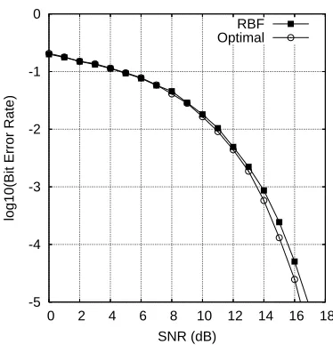
-5 -4 -3 -2 -1 0
0 2 4 6 8 10 12 14 16 18
log10(Bit Error Rate)
[image:3.595.330.517.73.267.2]SNR (dB) RBF Optimal
Figure 1: BER performance of the symmetric RBF and the Bayesian equaliser for transmission over a two-tap channel using an equaliser order ne=2 and a decision delayτ=1.
The OFS aided FRCSM algorithm was used.
For the RBF equaliser (23) using the Gaussian basis func-tion of (10), the derivatives of the RBF network’s output with respect to the RBF equaliser’s parameters are given by
∂yRBF
∂θi =e
−kx(k)−µik2
ρ2
i −e−
kx(k)+µik2
ρ2
i ,
∂yRBF
∂ρ2
i
=θi e
−kx(k)−µik2
ρ2
i kx(k)−µik
2
(ρ2
i)
2 −e
−kx(k)+µik2
ρ2
i kx(k)+µik
2
(ρ2
i)
2
! ,
∂yRBF
∂ µi =θi e
−kx(k)−µik2
ρ2
i x(k)−µi
ρ2
i
+e−
kx(k)+µik2
ρ2
i x(k)+µi
ρ2
i !
,
(30) for 1≤i≤M.
4. SIMULATION STUDY
Example 1. The two-tap CIR used was given by x(k) =
0.5b(k) +1.0b(k−1) +n(k), the equaliser order was set to
ne=2 and the decision delay to τ=1. Fig. 1 shows the
BER of the optimal Bayesian equaliser as a function of the
-2 -1.5 -1
0 2 4 6 8 10
log10(Bit Error Rate)
[image:3.595.329.518.567.698.2]Model Size RBF Bayesian
Figure 2: Influence of the model size on the BER perfor-mance for transmission over a two-tap channel in conjunc-tion with ne=2 and τ=1, given SNR=10 dB. The OFS
-2 -1
0 40 80 120 160 200 240 280 320
log10(Bit Error Rate)
[image:4.595.73.261.66.203.2]Data Size RBF Bayesian
Figure 3: Influence of the data length on the BER perfor-mance for transmission over the two-tap channel in conjunc-tion with ne=2 and τ=1, given SNR=10 dB. The OFS
aided FRCSM algorithm was used.
-2 -1
0.1 1 10 100
log10(Bit Error Rate)
[image:4.595.330.515.268.455.2]RBF variance/noise variance RBF Bayesian
Figure 4: Influence of the RBF variance on the BER perfor-mance for transmission over the two-tap channel in conjunc-tion with ne=2 and τ=1, given SNR=10 dB. The OFS
aided FRCSM algorithm was used.
signal to noise ratio (SNR). For this example, the size of the Bayesian equaliser was defined by Nsb=4. For each
SNR, a symmetric RBF equaliser having a Mspa=4 was constructed from the training data set of length K=160 us-ing the OFS aided FRCSM algorithm, and the BER perfor-mance of the resultant RBF equaliser is also plotted in Fig. 1. Given SNR=10 dB and a training data length of K=160, Fig. 2 depicts the influence of the RBF model size Mspa on the attainable BER performance, where the RBF varianceρ2 was tuned for each model size and was in the range of σn2 to 4σ2
n. At SNR=10 dB, a model size of Mspa=4 and the RBF variance ofρ2=2σ2
n, the influence of the data length K is plotted in Fig. 3, while Fig. 4 illustrates the influence
of the RBF varianceρ2given SNR=10 dB, Mspa=4 and
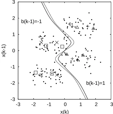
K =160. Fig. 5 compares the optimal Bayesian decision boundary with that of the RBF equaliser, given SNR=10 dB.
Example 2. The three-tap CIR was given by x(k) =
0.3b(k) +0.8b(k−1) +0.3b(k−2) +n(k), the equaliser or-der was set to ne=4 and the decision delay wasτ =2.
The BER of the optimal Bayesian equaliser is depicted in Fig. 6. For this example, the size of the Bayesian equaliser was defined by Nsb=32. Given SNR=13 dB and a model
size of M=30, Fig. 7 shows the learning curve ˜PE(w(k))
of the NLBER algorithm averaged over 10 runs, where the BER was estimated using a block size of K =500 sym-bols and a kernel variance of σ2=σ2
n. The NLBER
al-gorithm having a step sizeξ =0.1 was initialised with the first 30 data points as the initial RBF centres, and we had
ρ2
i(0) =4.0σn2 and θi(0) = 301 for 1≤i≤30. The true
BER PE(w(k)) was also calculated using simulations for K=0,400,800,1200,1600,2000. Fig. 8 depicts the influ-ence of the model size on the RBF equaliser’s performance, where the NLBER algorithm had the same settings as those used for obtaining the results of Fig. 7. The BER of the RBF equaliser using the model size of M=30, trained by the NLBER algorithm over K=2000 samples is also shown in Fig. 6.
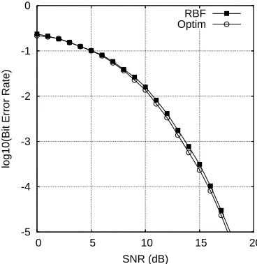
The OFS aided FRCSM algorithm was also used to se-lect the RBF equaliser having a model size of Mspa=30 in conjunction with the training block length of K =600 and the RBF variance ofρ2=σ2
n. The BER performance of the
resultant RBF equaliser is depicted in Fig. 9, in comparison to the performance of the Bayesian equaliser.
-3 -2 -1 0 1 2 3
-3 -2 -1 0 1 2 3
x(k-1)
x(k) b(k-1)=-1
[image:4.595.73.261.269.403.2]b(k-1)=1
Figure 5: Comparison of the decision boundaries (solid: Bayesian and dashed: RBF) for the two-tap channel in con-junction with ne=2 andτ=1, given SNR=10 dB, where
pairs of cross and plus symbols indicate the positions of metric state pairs, and the pairs of square and triangular sym-bols indicate the positions of RBF centre pairs. The OFS aided FRCSM algorithm was used.
5. CONCLUSIONS
In this paper, we have investigated a novel symmetric RBF network structure designed for channel equalisation applica-tion. As a benefit of the underlying symmetry property of the optimal Bayesian equalisation solution, we were able to ap-proach the optimal Bayesian performance using noisy train-ing data. Both a block-data based and a sample-by-sample adaptive training algorithm have been proposed for this sym-metric RBF equaliser, and the simulation results have in-dicated that they are capable of approaching the optimum Bayesian performance.
REFERENCES
-5 -4 -3 -2 -1 0
0 5 10 15 20
log10(Bit Error Rate)
[image:5.595.74.258.67.257.2]SNR (dB) RBF Optim
Figure 6: Comparison of BER performance for the three-tap channel with equaliser order ne=4 and decision delayτ=2.
The NLBER algorithm was used.
1e-3 1e-2 1e-1 1
0 400 800 1200 1600 2000
Bit Error Rate
sample NLBER: Esti. BER NLBER: True BER Bayesian
Figure 7: Learning curve of the NLBER algorithm averaged over 10 runs for the three-tap channel with ne=4 andτ=2,
given SNR=13 dB.
[2] S. Chen, B. Mulgrew and P.M. Grant, “A clustering technique for digital communications channel equalisa-tion using radial basis funcequalisa-tion networks,” IEEE Trans.
Neural Networks, vol.4, no.4, pp.570–579, 1993.
[3] S. Chen, S. McLaughlin, B. Mulgrew and P.M. Grant, “Adaptive Bayesian decision feedback equaliser for dis-persive mobile radio channels,” IEEE Trans.
Communi-cations, vol.43, no.5, pp.1937–1946, 1995.
[4] S. Chen, S.R. Gunn and C.J. Harris, “The relevance vector machine technique for channel equalization ap-plication,” IEEE Trans. Neural Networks, vol.12, no.6, pp.1529–1532, 2001.
[5] A. Wolfgang, S. Chen and L. Hanzo, “Radial basis function network assisted space-time equalisation for dispersive fading environments,” Electronics Letters, vol.40, no.16, pp.1006–1007, 2004.
[6] S. Chen, B. Mulgrew and L. Hanzo, “Asymptotic Bayesian decision feedback equalizer using a set of hyperplanes,” IEEE Trans. Signal Processing, vol.48, no.12, pp.3493–3500, 2000.
[7] K.Z. Mao, “RBF neural network center selection based on fisher ratio class separability measure,” IEEE Trans.
Neural Networks, vol.13, no.5, pp.1211–1217, 2002.
-3 -2 -1
5 10 15 20 25 30 35 40
log10(Bit Error Rate)
[image:5.595.330.517.68.201.2]Model Size RBF Bayesian
Figure 8: Influence of the model size to the BER perfor-mance for the three-tap channel with ne=4 andτ=2, given
SNR=13 dB. The NLBER algorithm was used.
-5 -4 -3 -2 -1 0
0 5 10 15 20
log10(Bit Error Rate)
SNR (dB) RBF Optim
Figure 9: Comparison of BER performance for the three-tap channel with equaliser order ne=4 and decision delayτ=2.
The OFS with FRCSM algorithm was used.
[8] S. Chen, L. Hanzo and A. Wolfgang, “Kernel-based nonlinear beamforming construction using orthogonal forward selection with Fisher ratio class separabil-ity measure,” IEEE Signal Processing Letters, vol.11, no.5, pp.478–481, 2004.
[9] S. Chen, L. Hanzo and A. Wolfgang, “Nonlinear multi-antenna detection methods,” EURASIP J. Applied
Sig-nal Processing, vol.2004, no.9, pp.1225–1237, 2004.
[10] E. Parzen, “On estimation of a probability density func-tion and mode,” The Annals of Mathematical Statistics, Vol.33, pp.1066–1076, 1962.
[11] B.W. Silverman, Density Estimation. London: Chap-man Hall, 1996.
[12] A.W. Bowman and A. Azzalini, Applied Smoothing
Techniques for Data Analysis. Oxford: Oxford
Univer-sity Press, 1997.
[13] S. Chen, B. Mulgrew and L. Hanzo, “Least bit error rate adaptive nonlinear equalizers for binary signalling,”
IEE Proc. Communications, vol.150, no.1, pp.29–36,
2003.
[14] R.O. Duda and P.E. Hart, Pattern Classification and
[image:5.595.331.515.246.435.2] [image:5.595.71.270.287.436.2]