Shadow Detection in Aerial Images using Machine Learning

(1)

Theses

7-30-2019

Shadow Detection in Aerial Images using Machine

Learning

Prasanna Reddy Pulakurthi

(2)

Machine Learning

by

Prasanna Reddy Pulakurthi

A Thesis Submitted in Partial Fulfillment of the Requirements for the Degree of Master of Science in Electrical Engineering

Supervised by

Dr. Emmett J. Ientilucci

Chester F. Carlson Center for Imaging Science Rochester Institute of Technology. Rochester, New York

July 30, 2019

Approved by:

Dr. Emmett J. Ientilucci, Assistant Professor

Thesis Advisor, Chester F. Carlson Center for Imaging Science

Dr. Majid Rabbani, Visiting Professor

Committee Member, Department of Electrical and Microelectronic Engineering

Dr. Eli Saber, Professor

Committee Member, Department of Electrical and Microelectronic Engineering

Dr. Sohail A. Dianat, Professor

(3)

Rochester Institute of Technology Kate Gleason College of Engineering

Title:

Shadow Detection in Aerial Images using Machine Learning

I, Prasanna Reddy Pulakurthi, hereby grant permission to the Wallace Memorial Library

to reproduce my thesis in whole or part.

Prasanna Reddy Pulakurthi

(4)

Dedication

(5)

Acknowledgments

I like to thank my advisor Dr. Emmett Ientilucci for the regular meetings and guidance

through each and every stage of this journey and also for inspiring my interest in

developing algorithms related to this thesis. I would also like to thank my committee

members, Dr. Majid Rabbani and Dr. Eli Saber, for their ideas and insights which also

helped to develop this thesis. Finally, I would like to thank the RIT EE department head,

Dr. Sohail, and my professor, Dr, Rabbani, for recommending me to professor Ientilucci

who ultimately introduced me to this research project.

This research was sponsored by Oak Ridge National Laboratory, managed by UT-Battelle,

(6)

Abstract

Shadow Detection in Aerial Images using Machine Learning

Prasanna Reddy Pulakurthi

Supervising Professor: Dr. Emmett J. Ientilucci

Shadows are present in a wide range of aerial images from forested scenes to urban

environments. The presence of shadows degrades the performance of computer vision

al-gorithms in a diverse set of applications such as image registration, object segmentation,

object detection and recognition. Therefore, detection and mitigation of shadows is of

paramount importance and can significantly improve the performance of computer vision

algorithms in the aforementioned applications. There are several existing approaches to

shadow detection in aerial images including chromaticity methods, texture-based

meth-ods, geometric, physics-based methmeth-ods, and approaches using neural networks in machine

learning.

In this thesis, we developed seven new approaches to shadow detection in aerial imagery.

This includes two new chromaticity based methods (i.e., Shadow Detection using Blue

Illumination (SDBI) and Edge-based Shadow Detection using Blue Illumination

(Edge-SDBI) and five machine learning methods consisting of two neural networks (SDNN and

DIV-NN), and three convolutional neural networks (VSKCNN, SDCNN-ver1 and SDCNN

ver-2). These algorithms were applied to five different aerial imagery data sets. Results

(7)

Conclusions touch upon the various trades between these approaches, including speed,

(8)

List of Contributions

• We coded and delivered algorithms, as mentioned in this thesis, to our sponsor.

• In this thesis, we proposed and developed the following seven methods for shadow

detection in areal images:

– Shadow Detection using Blue Illumination (SDBI).

– Edge based Shadow Detection using Blue Illumination (Edge-SDBI).

– Shadow Detection Neural Network (SDNN).

– Division-based Neural network (DIV-NN).

– Variable Sized Kernels Convolutional Neural Network (VSKCNN).

– Shadow detect Convolutional Neural Network Version1 (SDCNN-ver1).

– Shadow detect Convolutional Neural Network Version1 (SDCNN-ver2).

(9)

List of Figures

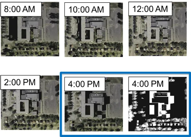
2.1 DIRSIG generated image at 12:00am. . . 9

2.2 DIRSIG generated images at different times of the day. Example shadow mask at 4:00pm (bottom right). . . 9

3.1 Notional layout of the shadow collection experiment. . . 13

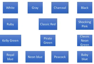
3.2 Various colored panels used in the shadow collection experiment. . . 14

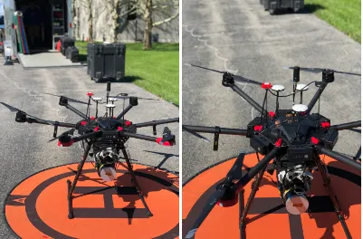
3.3 Drone used for the data collect. . . 15

3.4 Field images showing the target deployment and strong shadows from a tall building. . . 16

3.5 a) Nadir view of shadow collection experiment and b) zoomed in version showing the building and deployed targets in the shadow. . . 17

4.1 Example input image from the WV2 data-set. . . 20

4.2 SDBI output for the WV2 image of Figure 4.1. . . 21

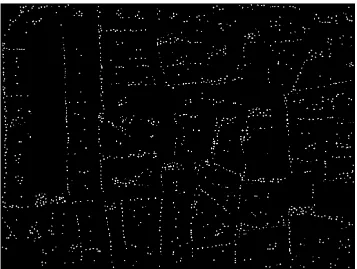
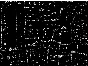
4.3 Edges from performing Canny Edge Detection on the L band. . . 22

4.4 Initially selected seeds. . . 22

4.5 Region growing after 2 iterations. . . 23

4.6 Final output after region growing and filling process. . . 24

4.7 Example WV2 image used to illustrate data selection. . . 25

4.8 Data chosen using the random selection method. . . 26

4.9 (a) Shadows classified into six different classes using k-means. (b) Non-shadow regions classified into eight classes using k-means. . . 27

4.10 Data chosen using the Balanced data selection method. . . 28

4.11 SDNN architecture . . . 29

4.12 Division-based Neural Network (DIV-NN) . . . 30

4.13 Division Network added to our SDNN . . . 31

4.14 (a) Typical input image. (b) Reference image. . . 33

4.15 (a) Preprocessed image after brightness matching to the reference image. (b) Reference image . . . 34

4.16 VSKCNN architecture. . . 35

(12)

4.18 Chips for training SDCNN from a WV2 image. . . 38 4.19 SDCNN-ver2 architecture. . . 39

5.1 (a) DIRSIG image, (b) WV2 image, (c) Valencia image, (d) UIUC image, (e) SC data image. . . 43 5.2 Output shadow mask of the three existing chromaticity shadow detection

methods. . . 44 5.3 Output shadow masks of the two proposed chromaticity shadow detection

methods. . . 46 5.4 Output shadow masks of the two proposed neural networks. . . 48 5.5 Output shadow masks of different Convolutional neural networks. . . 49 5.6 Heat map of quantitative metrics verses all the algorithms on the DIRSIG

data. Values in parenthesis are standard deviations. . . 51 5.7 Example Image 1: DIRSIG data. . . 52 5.8 Heat map of quantitative metrics verses all the algorithms on the WV2 data. 54 5.9 Example Image 2: WV2. . . 55 5.10 (a) Input UIUC image. (b) Hand labeled ground truth. . . 56 5.11 Heat map of quantitative metrics verses all the algorithms on the UIUC

data based on 50 images. . . 57 5.12 Example Image 4: UIUC. . . 58 5.13 Heat map of quantitative metrics verses all the algorithms on the Shadow

(13)

Chapter 1 Introduction

In this thesis we would like to address the problem of shadows in aerial images. We are

interested in shadow detection as shadows can cause problems while performing image

registration and other computer vision applications. Therefore, we wish to detect shadows

in aerial images.

We started by doing a literature review on existing shadow detection methods and built

upon some of the basic concepts. We developed two chromaticity methods. Furthermore,

we used machine learning concepts to address this problem. Building on the fundamentals

of machine learning, we proposed five simple machine-learning algorithms. The neural

networks proposed in this thesis have high computational speed. We then compare the

performance of all the different methods proposed in the thesis using qualitative and

(14)

Chapter 2 Background

2.1 Existing Approaches to Shadow Detection in Areal Imagery

2.1.1 Chromaticity Methods

Chromaticity is one of the most popular methods to perform shadow detection. In this

method shadow detection is based on spectral information. That is, RGB (Red, Green and

Blue bands) and sometimes the Near IR bands. These methods work on the assumption

that the regions in shadows become darker and the shadowed regions preserve the

chro-maticity information of the underlying material. For instance, green vegetation in shadow

would sill contain the same spectral information but just look darker. This color model,

where the intensity reduces but the chromaticity remains unchanged, is generally referred

to as colour constancy [22] or linear attenuation [23]. Methods that use this approach

gen-erally use a different color space so as to have a better separation between chromaticity

and intensity than using RGB space (example color spaces include HSV[26], c1c2c3[30],

YUV[24]). These algorithms are generally simple to implement and computationally

in-expensive. However, these algorithms perform pixel-level analyses and are prone to noise

[25]. They are also sensitive to the strength of shadows, as shadows can be strong on a

sunny day with clear skys or weak on a cloudy day. The following subsections explain

(15)

Normalized Saturation Value Difference Index (NSVDI)

Ma et. al. [28] proposed a shadow detection method by working in Hue Saturation Value

(HSV) color space. First, an RGB image is converted to HSV space. We then find the

NSVDI as,

N SV DI = S−V

S+V (2.1)

where S and V are the normalized saturation and value components, respectively. A

positive threshold T is applied on NSVDI to create a binary shadow mask. This threshold

is set to be zero. The image pixel is labeled as a shadow pixel if the NSVDI is greater than

threshold T; else, it is non-shadow.

Shadow Detection Index (SDI)

The Shadow Detection index, proposed by Y. Mostafa [29], makes use of four bands: red,

green, blue and NIR. Here are the observations made by Y. Mostafa [29] in shadowed

regions.

1) In shadows, the intensity of the red band decreases sharply.

2) Intensity values of shadow and non-shadow areas have the smallest difference in the

blue band.

3) Smaller values for the term (G-B) in shadows.

4) Shadow pixels have low difference between green and blue bands. Larger differences

(16)

From these observations, the SDI is developed. For every pixel, the SDI is calculated

using

SDI = (1−PC1)+1

((G−B) ∗R)+1 (2.2)

where, R, G and B are the normalized values of the red, green and blue bands,

respec-tively. PC1 is the normalized first principal component. Principal component analysis is

performed on the red, green, blue and NIR bands. The first principal component contains

most of the information and gives a very good estimate for the brightness in the image. SDI

is formed from four different bands R, G, B and PC1. These are used in a way to

maxi-mize SDI in shadows with a minimum score in non-shadows. PC1 produces low values in

shadows; therefore,(1−PC1)is used in the numerator. From observations 1) and 3) above

((G − B) ∗ R)has low values in shadows, therefore we use this term in the denominator.

Then a one is added in the numerator and denominator for stability. Finally, the SDI output

is stretched to fit the range (0-255). Then a subjective threshold T is used to binarize and

create a shadow mask.

C3 Index

This algorithms is developed using a function on the ratio of bands. The C3 index from

[30] uses arctan on the ratio of the blue band and maximum of green and red bands. This

is seen in Equation (2.3).

C3=arctan

B

max(G,R)

(17)

Due to atmospheric Rayleigh scattering effects, shadow pixels are typically saturated

with short blue wavelengths. Therefore, the C3 index emphasises the blue component in

the numerator. Due to the high emphasis on the blue band, most of the blue regions, like

water and some blue objects, are misclassified as shadows.

2.1.2 Texture-based Methods

based methods exploit the fact that texture is retained in shadowed regions.

Texture-based methods generally are implemented in two steps: 1) Finding candidate shadow pixels

or regions, and 2) classifying them into either foreground or shadows. In the first step,

shad-ows are selected based on spectral features. Then each shadow candidate region is classified

as an object or shadow by checking the texture. If two regions have different spectral

char-acteristics but the same texture information, then we choose the region with lower intensity

as the shadowed region. Different types of correlation techniques are proposed (e.g. Gabor

filtering [1]), Markov or conditional random fields [2, 3], orthogonal transforms [4],

gradi-ent or edge correlation [5, 6, 7], normalised cross-correlation [8]). Texture-based methods

can be powerful because textures are highly distinctive. Also, these methods are robust to

change in illumination. However, texture-based methods are typically slow as they

com-pute several neighborhood comparisons for each pixel. Hence, we did not explore this

method as we are looking for methods that have faster run times.

2.1.3 Geometric Based Methods

With prior knowledge of source illumination and object shape, we can predict the

orien-tation, size and shape of the object. This information is used by some methods to split

(18)

directly with input frame data and does not rely on an accurate estimate of the background

reference. However, geometric based methods have scene limitations such as: they require

specific object types, vehicles [10, 13] or pedestrians [9, 11] and assume that the source

of light is unique [12] or the background surface is flat [10]. Moreover, current geometric

based algorithms cannot deal with multiple shadows from a single object. This method

is not applicable to aerial images as we do not have the prior knowledge related to the

direction of illumination or the objects in the scene.

2.1.4 Physical Methods

Linear attenuation models make an assumption that the illumination source is purely white

[14], which is often not true. In a typical outdoor environment, the two major sources of

illumination are the sun and the light reflected from the blue sky. The light from the sun

generally dominates any other light source. However, when the sunlight is blocked

(creat-ing shadows), the main source of light is the light from the sky, which is typically blue due

to the atmospheric Rayleigh scattering effect. A dichromatic model was employed in [14]

which takes into account both of these illumination sources to better estimate shadowed

re-gions. Other non-linear attenuation models are proposed [15, 16] which account for various

illumination conditions in a variety of indoor and outdoor scenarios. Alternatively, some

methods learn the appearance of all the pixels in shadows for shadow detection without

nec-essarily proposing any particular model [17, 18, 19]. These methods or models that try to

learn the appearance of the shadowed regions are referred to as physical approaches. These

methods are more accurate than chromaticity methods (comparisons reported in [17, 18]).

(19)

similar chromaticity to that of the fully illuminated objects. Hence we did not use this

approach.

2.1.5 Existing Machine Learning Approaches to Shadow Detection

Shadow detection, using visible light surveillance cameras, is proposed in [20]. This

method used a convolutional VGG Net-16 architecture for shadow detection. Fast shadow

detection using patched convolutional networks were used in [21]. This method uses

tex-ture and color featex-tures to produce a shadow prior map. This is then used along with the

RGB image to create an output shadow mask using RGBP CNN (RGBP is RGB stacked

with Prior map these are used as input for the RGBP CNN), as described in their work.

Shadow detection using conditional Generative Adversarial Networks (cGAN) was

pro-posed in [32]. GANs use a generator and a discriminator. A generator produces images to

fool the discriminator and the discriminator’s job is to correctly classify real images (i.e,

real input images) from fake ones (generated by the generator). The cGANs use an input in

the generator to produce the fake image. In this method, the authors used the generator to

create the shadow mask. The discriminator is given the input image along with the shadow

mask. The training is stopped when the discriminator cannot discriminate between real

and fake images. This is because the generator has become good in generating the shadow

mask, that is indistinguishable from the ground truth (GT). In the end, this generator is used

for shadow detection.

We have designed our Neural Networks and Convolutional Neural Networks, building

(20)

We did not test these machine learning algorithms in the literature against our proposed

ma-chine learning methods because we could neither obtain the source code of these algorithms

from the authors nor did we have enough time to write our own code for implementing these

methods.

2.2 Data

For analyzing and testing the performance of different algorithms, we used five different

data-sets which are described in the following sections.

2.2.1 DIRSIG

Working with neural networks demands data. We generated RGB synthetic images and

their corresponding shadow masks using the digital imaging and remote sensing image

generation (DIRSIG) model [33].

The DIRSIG model is a physics-driven synthetic image generation model developed by

the Digital Imaging and Remote Sensing Laboratory in the Center for Imaging Science

at Rochester Institute of Technology. The model can produce passive single-band,

multi-spectral or hyper-multi-spectral imagery from the visible through the thermal infrared region of

the electromagnetic spectrum. The model also has a very mature active laser (LIDAR)

capability and an evolving active RF (RADAR) capability. The model can be used to test

image system designs, to create test imagery for evaluating image exploitation algorithms

and for creating data for training image analysts.

A sample image produced using the DIRSIG model is shown in Figure 2.1. We used

(21)

[image:21.612.155.467.94.393.2]

Figure 2.1: DIRSIG generated image at 12:00am.

[image:21.612.156.463.435.655.2]

(22)

can help produce different sized shadows. For instance, large shadows are produced during

dusk and dawn while short ones are produced during noon. A large portion of these images

contain vegetation while only a few regions contain large buildings. Any imagery used in

future sections of this document will be referred to as a DIRSIG image.

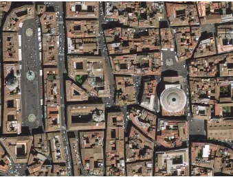
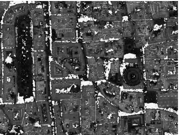
2.2.2 WorldView-2 (WV2)

WorldView-2 is a commercial Earth observation satellite that captures aerial images. We

selected the RGB images produced by this satellite which were available to use [34]. We

obtained 20 images from WV2 and created shadow masks for 6 images. In the following

sections, we refer to all the WorldView-2 images as the WV2 image. This data consists of

a variety of regions containing vegetation, asphalt, buildings and cities.

2.2.3 University of Illinois at Urbana-Champaign (UIUC) Data

The University of Illinois at Urbana-Champaign has created an image data-set [35] along

with their corresponding masks. We used 50 aerial images from this data-set for testing

our algorithms. These data-sets contain varying textures as well as different materials in

shadow and non-shadowed regions.

2.2.4 Shadow Collect Data (SC data)

We performed a shadow collect consisting of different colored targets placed in shadow and

non-shadowed regions. Chapter 3 contains a detailed explanation of this shadow collect.

(23)

2.3 Methods to Evaluate Success

Other than visually analyzing the shadow detection output, it would be helpful to have a

quantitative metric to access the performance of an algorithm. For this research, we will use

Completeness, Correctness, Quality and Accuracy metrics, which were originally proposed

by Wiedemann et al. (1998) and adopted in [36]. These metrics will verify which approach

is best at finding shadows and also avoid misclassifications. Thus, we compare the detected

result with the ground truth, pixel-wise. All the quantitative metrics have a range of values

from zero to one (0 to 100 percent) and are utilized in Chapter 5 of this thesis.

2.3.1 Completeness

The fist metric, called completeness (Com), is the percentage of shadow pixels in the

ground truth (GT) that were properly detected. Completeness is found using,

Com= T P

T P+F N (2.4)

where, TP are true positives (number of shadow pixels correctly detected as shadow)

and FN are false negatives (which are the number of GT shadow pixels that are classified

as non-shadows). In signal processing, TP is often referred to as detects (D) and FN is

referred to as misses (M).

2.3.2 Correctness

The correctness (Cor) metric is the percent of shadow detects that are correctly identified

using the methods in reference to the GT. The correctness metric is given by,

Cor = T P

(24)

where, FP are false positives (number of non-shadow pixels that are classified as shadow).

FP are sometimes referred to as False Alarms (FA).

2.3.3 Quality

The Quality (Qua) metric combines both of the previous metrics and is given by,

Qua= T P

T P+F P+F N (2.6)

This metrics tells us how good the method is. Where a higher value reflects better

algorithmic performance with the highest achievable value being one.

2.3.4 Accuracy

The accuracy (Acc) metric is the percentage of shadows and non-shadows classified

cor-rectly and is given by,

Acc = T P+T N

T P+F P+T N+F N (2.7)

(25)

Chapter 3 Shadow Collection Experiment

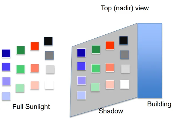
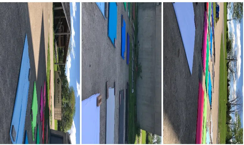
The objective of the shadow experiment was to create a controlled shadow collection

con-taining different gradients of color in shadow and non-shadows, as shown in Figure 3.1.

This should create a very difficult shadow detection data-set since there are very bright

objects in shadows and very dark objects in full illumination.

On May 21st 2019, with the help of the unmanned aerial system (UAS) data collection

team at the Rochester institute of technology, we conducted the actual data collect. We

[image:25.612.122.424.468.679.2]

placed the first set of panels, containing 14 different colors, in shadows and another set of

(26)

[image:26.612.113.508.82.351.2]

Figure 3.2: Various colored panels used in the shadow collection experiment.

the same 14 colored panels in full illumination. A list of the colors used is shown in Figure

3.2. Additionally we placed two sets of felt on plywood (containing light grey, medium

grey and black) which were used for calibration.

The drone in Figure 3.3, is called the MX1 which is RITs multi-model UAS platform.

This system contains five different imaging systems namely Headwall nano, Mako G419,

Tamarisk 640, Velodyne lidar and multispetral Micasense camera. With these imaging

systems, we obtained RGB, multi-spectral, hyper-spectral, lidar and thermal images.

We flew two missions, one at 10:38 am another at 11:06 am local time. The weather

conditions were mostly sunny with a few fast moving clouds. The center of the scene

contained a three story building. This building produced strong shadows, as seen in Figure

(27)

[image:27.612.110.511.90.354.2]

Figure 3.3: Drone used for the data collect.

During mission 1106, all MX1 sensors recorded data. Spectral reflectance and radiance

measurements of the targets, both in full sun and shadow, were recorded. The raw data

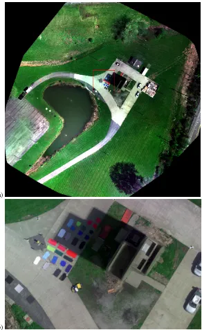
was both geometrically corrected and calibrated to radiance. Figure 3.5 shows one of the

(28)

[image:28.612.116.505.269.501.2]

(29)

a)

[image:29.612.166.458.139.615.2]

b)

(30)

Chapter 4 New Approaches to Shadow Detection

In this chapter, we propose and describe a total of seven different approaches to shadow

de-tection. This includes two chromaticity based methods (SDBI and Edge-SDBI), two

Neu-ral networks (SDNN and DIVNN) and three Convolutional NeuNeu-ral Networks (VSKCNN,

SDCNN-Ver1 and SDCNN Ver-2). These methods are presented in the following sections.

4.1 Chromaticity Methods

This section gives a detailed description of the proposed chromaticity methods entitled

SDBI and Edge-SDBI.

4.1.1 Shadow Detection using Blue Illumination (SDBI)

The Blue Illumination shadow detection method is built from a well established observation

that shadows contain a fair amount of blue light. The idea is to give high priority to the

blue band, at the expense of picking blue objects such as water or blue buildings. These

miss-classified (i.e. false alarm) blue pixels generally have a higher intensity than all of

the shadow regions, hence we use the the lightness component in the Lab color space to

remove these miss-classified pixels.

The idea is to output a high value for false alarmed blue pixels and low values for all

(31)

finally present our work on the best working formulation, as show in Equation (4.1).

SDBI = 1− B

max((1−b),R) (4.1)

where R andB are the normalized values of the Red and Blue channels respectively. bis

the b-component in CIE Lab space. That is, Lab space has three components, L* for the

lightness from black (0) to white (100), a* from green (-) to red (+), and b* from blue (-)

to yellow (+). The ratio of B band and the maximum of (1-b) and R produces low values

for shadow, therefore, one minus this term produces a high output value for shadow pixels.

We observe that the output of SDBI in the shadowed regions is very close to one.

There-fore, to classify we use the condition that, a pixel is a shadow if SDBI is greater than

thresholdTBI. Empirically we found the best results using a threshold of 0.9. When we

observe that some of the blue pixels are miss-classified as shadows, we remove these using

the L component of the Lab space. A threshold-based approach using the L component is

presented in [31], in which a pixel is classified as shadow if the L component is less than

TL. This thresholdTL is found using Equation (4.2) where a pixel is considered shadow if

it satisfiesSDBI > 0.9 and L <TL.

TL = µL −

1

3 ∗σL, (4.2)

(32)

[image:32.612.141.480.88.346.2]

Figure 4.1: Example input image from the WV2 data-set.

4.1.2 Edge based Shadow Detection using Blue Illumination (Edge-SDBI)

V. Arevalo [26] proposed a method of using both the chromaticity and edges for finding

shadows. Our implementation makes use of the SDBI given in Section 4.1.1 and edges

to guide the region growing. The steps of the algorithm are described below along with

example WV2 imagery.

1. Image-preprocessing: The WV2 image is shown in Figure 4.1. The following

com-ponents are computed and used in step 2 of the algorithm.

(a) RGB image is converted to Lab color space. ThresholdTL is found using

Equa-tion (4.2).

(b) SDBI is computed as described in Section 4.1.1. The computed SDBI is shown

(33)

[image:33.612.132.489.88.356.2]

Figure 4.2: SDBI output for the WV2 image of Figure 4.1.

(c) Perform Canny Edge Detection [27] on the L channel to obtain a edge component

E. The edges can be seen in the Figure 4.3.

2. Seed Selection: A pixel is selected as a seed if it has a high chance of being a shadow

pixel. The following conditions are used to label a pixel as a seed.

(a) The SDBI value of the pixel must be the local maximum of a 9×9 neighborhood.

(b) The mean of a 9×9 neighborhood of the L component is computed. This value

must be less than the thresholdTL.

(c) Only one seed can exist in a 9×9 neighborhood.

After applying the above conditions, initial seeds are selected. The results of this

(34)

[image:34.612.131.490.91.363.2]

Figure 4.3: Edges from performing Canny Edge Detection on the L band.

[image:34.612.132.489.403.672.2]

(35)

[image:35.612.131.488.87.355.2]

Figure 4.5: Region growing after 2 iterations.

3. Region Growing and filling: After the initial seeds are selected, we start region

grow-ing. A pixel is considered shadow and added to the seed if it satisfies the following

conditions:

(a) The L value of the corresponding pixel must be less thanTL.

(b) The region stops growing when it reaches the edges.

Figure 4.5 shows the growing process in the second iteration. Regions are grown until

they reach convergence (next iteration produces the same result).

The final filling process is done using morphological image processing. We perform

a dilation followed by an erosion using a 3×3 filter. The final output, after complete

(36)

Figure 4.6: Final output after region growing and filling process.

4.2 Neural Networks

In this section, we describe the two neural network based methods namely, Shadow

De-tection Neural Network (SDNN) and Division-based Neural network (DIV-NN). However,

we first describe the input data used for these neural networks.

4.2.1 Choosing Input data for the Neural Networks

The inputs for the neural networks are the RGB values. We explored two ways of choosing

the data for training the Neural Networks, random selection and balaned data selection.

Random Selection

In this method we randomly choose RGB pixels from a given training image. This method

(37)

Figure 4.7: Example WV2 image used to illustrate data selection.

method is that, the data is more scene dependent. We want our data to have a lot of variance

and contain all the scenarios that we would experience in the real-world. For example,

consider a training image in which a majority of the image is covered by vegetation. By

randomly choosing the data (by data we mean RGB pixel values) we will have unbalanced

data with more emphasis on vegetation. To overcome this we can use a balanced data

selection technique as described in the next subsection.

We illustrate an example for random selection using the WV2 image as seen in Figure

4.7. From this image, 40,000 pixels are chosen with 20,000 in shadow and 20,000 in

non-shadowed regions (this is done with the help of ground truth (GT) shadow mask). For

visual representation, this data is reshaped into an image of size 200×200 and shown in

(38)

Figure 4.8: Data chosen using the random selection method.

Balanced Data Selection

Balanced data selection helps choose equal amounts of data from different regions in

shad-ows and non-shadshad-ows. We first divide the original image into shadow and non-shadow

images using the help of GT, then apply k-means clustering on the shadow image and

non-shadow imagery. Then we randomly choose from each class, this ensures that we pick

equal amounts of data from all of the regions.

Using the same WV2 image from Figure 4.7, we first divide the image into shadow and

non-shadowed images using the shadow mask (GT). The shadow image is further divided

into six classes using k-means clustering as shown in Figure 4.9 (a). The non-shadowed

regions are divided into eight classes as shown in Figure 4.9 (b).

(39)

6 Shadows classes

(a)

8 Non-Shadows classes

(b)

Figure 4.9: (a) Shadows classified into six different classes using k-means. (b) Non-shadow regions classified into eight classes using k-means.

4.10. This data should contain equal amounts of all the regions and hence excludes the

possibility of data being dominated by a particular type of data. We observe faster

conver-gence when training the neural network using data from this method. However, this method

is slow due to the high time complexity for running k-means clustering algorithms on large

(40)

Figure 4.10: Data chosen using the Balanced data selection method.

4.2.2 Shadow Detection Neural Network (SDNN)

The architecture of our Shadow Detection Neural Network is shown in the Figure 4.11.

Training process: The input image is first made to have zero mean and unit variance.

Then we select 40,000 input RGB pixels with equal split of shadow and non-shadow pixels

using the random selection method as discussed in Section 4.2.1.

This randomly selected data is then reshaped into a column vector, so as to produce

input data matrix X of size 40,000×3. This input is stored in matrix X. X is multiplied

with weightsw1 and added to a biasb1 to produce the hidden layer outputHwith 16 nodes.

A sigmoid activation function is applied on H to produce Hsig. The hidden layer Hsig is

(41)

Figure 4.11: SDNN architecture

is applied onY to produce the final outputYsig. This above description can be written as

Hsig(n,16) =sigmod[X(n,3) ∗w1(3,16) +b1(1,16)] (4.3)

Ysig(n,1) = sigmod[Hsig(n,16)∗w2(16,1)+b2(1,1)] (4.4)

where X(n,3) is the input RGB reshaped matrix, w1 and w2 are the weights of the first

and second layer respectively, b1 and b2 are the bias terms of the first and second layers.

Hsig is the hidden layer output after sigmoid activation is applied. Ysig is the final layer

output after sigmoid activation. The final output has values ranging from zero to one (one

(42)

A mean squared error cost function is used. To minimize this cost function, all the

derivatives are found. The weights and bias are updated using gradient descent.

Implementation: The given test image is normalized to have a mean of zero and

vari-ance of one. Then the data is reshaped into the matrix X. This matrix value is fed to the

network and produces Ysig as described in the training process. This output Ysig is then

thresholded at 0.5 (i.e classify as a shadow pixel ifYsig>0.5) to produce the final shadow

mask. This shadow mask is in column form. We then have to resize this to the original

image dimensions. Since the network is trained to output a one for shadow and zeros for

non-shadows, it is a good idea to choose the threshold in-between the two values, hence we

choose the threshold to be 0.5.

4.2.3 Division-based Neural network (DIV-NN)

Since most of the chromaticity methods used some kind of a ratio or division, we

exper-imented by using a division network, as shown in Figure 4.12. We would like to see if

adding this architecture to our network would help for shadow detection over our simple

SDNN (previously described in Section 4.2.2).

(43)

Division Network: The Division network shown in Figure 4.12 is a ratio of linear

com-bination of Red, Green and Blue components. The equation for our Division network is

Divnet = sigmodR∗w1+G∗w2+B∗w3 R∗w4+G∗w5+B∗w6

(4.5)

where w1 to w6 are the weights to be learned. This network is added to our SDNN with

[image:43.612.114.501.260.552.2]

8 hidden layer nodes, as shown in Figure 4.13.

Figure 4.13: Division Network added to our SDNN

Training: The training procedure is similar to that of the SDNN. The mean normalized

unit variance data is given to the network. The hidden layer output consists of a

concatena-tion of both SDNN and the division network. These outputs are multiplied by weight w2

(44)

Ysig. Similar to the SDNN, a mean square cost function is used. All the derivatives are

found while the weights and bias are updated using gradient descent.

The same procedure, as described in the SDNN Section 4.2.2, is used for testing. The

image is mean normalized, reshaped and inputted to the network to get a probability output.

Similar to the SDNN method, we select a threshold of 0.5 to create a binary shadow mask

where one represents a shadow and zero represents a non-shadow.

4.3 Convolutional Neural Networks

In this section we describe three convolutional neural networks built for shadow detection

namely, Variable Sized Kernels Convolutional Neural Network (VSKCNN) and Shadow

detect Convolutional Neural Network Version1 and Version2 (ver1 and

SDCNN-ver2). However, we first describe the image preprocessing for matching the brightness for

all the training and testing images used in CNNs. The input images for CNNs are in the

scale from zero to one. We found through experimentation that this helps in faster training

of the CNNs.

4.3.1 Image-Preprocessing for Brightness Matching

Before we start the process, we identify one of the input images as a ‘reference image’

as shown in Figure 4.14 (b). This reference image has reasonable dynamic range (should

not have very high contrast and none of the regions should be clipped due to saturation)

and brightness. All other images are then scaled to match the mean and variance of this

reference image.

(45)

[image:45.612.103.526.86.289.2]

(a) (b)

Figure 4.14: (a) Typical input image. (b) Reference image.

like the reference image (in terms of mean and variance), as shown in Figure 4.14 (b), we

use,

Out put =

Input− µ_Im_g

σImg

×σr e f +µr e f (4.6)

where, µImgis the mean of the image, σImg is the standard deviation of the image, µr e f

is the mean of the reference image andσr e f is the standard deviation of the reference image.

In the case of RGB images we propose the following steps to be used:

Step 1: Change to YCbCr color space (the motivation in choosing YCbCr color space

is that, the Y band is a good representation of the illumination in the image. Moreover, any

operation performed on the Y band does not affect the spectral content of the image).

Step 2: Apply the above equation to the Y band.

Step 3: Convert back to RGB color space.

For the reference imagery in Figure 4.14 (b) which is re-scaled to fit a range (0,1), we

(46)

(a) (b)

Figure 4.15: (a) Preprocessed image after brightness matching to the reference image. (b) Reference image

we produce the preprocessed output image as shown in Figure 4.15 (a). We can observe the

preprocessed image has a higher brightness than the input image and matches in brightness

with the reference image.

4.3.2 Variable Sized Kernels Convolutional Neural Network (VSKCNN)

With this method, we used different size kernels to help capture different size features.

The architecture of “Variable Sized Kernels Convolutional Neural Network (VSKCNN)" is

shown in the Figure 4.16.

To explain the forward pass let us use an example image chip of size 240× 240×3

as shown in Figure 4.16. The first layer of this network contains four different size filters

7×7, 5×5, 3×3 and 1×1, eight filters each. Therefore, a total of 32 filters are used to

create the first layer output, called the hidden layer, which is of size 234×234× 32. A

leaky Rectified Linear Unit (ReLU) activation function is applied on this hidden layer. For

(47)

Figure 4.16: VSKCNN architecture.

The final layer output is created form a sum of up-convolutions of the first 8 hidden

layer outputs and 7×7×8 filter of the second layer. Next is 8 hidden layer outputs and a

5×5×8 filter followed by 8 hidden layer outputs and a 3×3×8 filter. The last 8 hidden

layer outputs is convolved by a 1×1×8 filter. The up-convolution operation produces a

similar dimension output as a deconvolution. In mathematics, deconvolution is a process

to reverse the effects of convolution. The way we produce the output is by resizing the

image such that the convolution output would produce the same output size as that of a

deconvolution. For example, if we perform a deconvolution on an image of size 234×234

using a filter of size 7×7, the output would be 230×230. Therefore in up-convolution, we

resize the image to be 246×246, so that when convolved with 7×7 produces an output of

size 230×230.

A sigmoid activation function is used on the final output to create an output shadow

probability which is in the range of zero to one. In this case, one represents shadows and

(48)

Training process: The input images are changed every 20 iterations. A input image

goes though the forward pass, as described above, and produces an output mask with the

same dimensions as that of the input image. A mean squared cost function is used and is

computed by taking the mean of the squared difference between the VSKCNN output and

the ground truth (GT). To minimize this cost function, the derivatives of all the variables

with respect to the cost function are found. The values of the different size filters are

updated using gradient descent.

Implementation: The input image is first brightness pre-processed, as described in

Sec-tion 4.3.1. This brightness pre-processed image is used as input to the VSKCNN

net-work which produces a probability output mask (values between zero to one, zero for

non-shadow and one for non-shadows). We then apply a threshold of 0.5 where a pixel is classified

as shadow if the VSKCNN output is greater than 0.5.

4.3.3 Shadow Detect Convolutional Neural Network Version1 (SDCNN-ver1)

This method consists of two convolution layers followed by max-pooling layers and a fully

connected convolutional layer. In all the hidden layers, ReLU is used as the activation

func-tion. However the final output layer uses sigmoid to produce an output shadow probability.

The architecture for SDCNN-ver1 is given in Figure 4.17.

For an example illustration of the forward pass, let us consider a 30×30×3 sized input

chip. The first layer convolution consist of a 3×3×3 filter, with four such filters. This is

followed by a ReLU activation. This produces an output of size 28×28×4. We then use

a max-pooling with a window of two and stride of two. The max-pooling output is of size

(49)

Figure 4.17: SDCNN-ver1 architecture.

a ReLU operation. The output produced after the second convolution and ReLu operation

is of size 12×12×4. The second max-pooling layer has a window of size two and stride of

two. This produces an output of 6×6×4 which is used as input to the next layer. Now we

implement a fully connected convolution layer. This is done by using eight filters of size

6×6×4, followed by a ReLU operation. The output of this layer is 1×1×8. The final layer

uses a kernel of size 1×1×8 to produce a single output followed by a sigmoid activation.

Hence, the final output is a shadow probability in which one represents shadows and zero

represents non-shadows.

Training process: The input image values are scaled to a range of values from zero to

one. We then create image chips for training. We created 450 chips of size 30×30 from

each image with the help of the Ground Truth (GT). The image chips created from the

WV2 image are shown in Figure 4.18.

In Figure 4.18, the shadow chips are shown on the left and non-shadowed chips are

(50)

[image:50.612.113.512.88.289.2]

Figure 4.18: Chips for training SDCNN from a WV2 image.

final output is a single value, as shown in the architecture. This value, along with the

ground truth, is used for the cost function. The mean squared cost function is calculated.

To minimize this cost function, all the derivatives are found. The weights (convolutional

kernels) are updated using gradient descent.

Implementation: The input image values are scaled to a have a range from zero to

one. This image is then used as input to the network. The only difference is that while

implementing the network for test images we set the max-polling stride to one. Once the

input flows thorough all the layers, the output mask is thresholded to 0.5 to create a shadow

mask.

Using convolution methods, the shadow regions tend to over extent into the non-shadowed

regions. Therefore to get rid of these miss-classifications we implemented our idea of

re-gion shrinking. Rere-gions shrinking is similar to the morphological erode operation.

(51)

This condition of brightness is found using the L space and thresholdTL, as described in

Section 4.1.1.

4.3.4 Shadow Detect Convolutional Neural Network Version2 (SDCNN-ver2)

This method is similar to SDCNN-ver1, which was described in Section 4.3.3. However,

the architecture is different with a higher number of filters in the hidden layers and the

method of training the network is also different. The architecture of the SDCNN-ver2 is

shown in Figure 4.19.

Figure 4.19: SDCNN-ver2 architecture.

For an example illustration of the forward pass, let us consider a 30×30×3 sized input

chip. The first layer convolution consist of a 3×3×3 filter, with four such filters, this is

followed by a leaky ReLU activation. This produces an output of size 28×28×4. Then we

use a max-pooling with a window of two and stride of two. The max-pooling output is of

size 14×14×4. The second convolution layer consists of four filters of size 5×5, followed

(52)

ReLu operation is of size 10×10×8. The second max-pooling layer has a window of size

two and stride of two, this produces an output of 5 ×5×8 which is used as input to the

next layer. Now we implement a fully connected convolution layer. This is done by using

24 filters of size 5×5×8, followed by a leaky ReLU operation. The output of this layer

is 1 ×1× 24. The final layer uses a kernel of size 1× 1× 24 to produce a single output

followed by a sigmoid activation. Hence, the final output is a shadow probability in which

one represents shadows and zeros represents non-shadows.

The difference between this network and the previous network, described in Section

4.3.3, is that ReLU is replaced by leaky ReLU. Instead of gradient descend, we used Adam

Optimize for faster convergence [37]. This new architecture of increased Kernels, increases

the performance of the network. Leaky ReLU and Adam Optimizer helps for faster

(53)

Chapter 5 Results

Results were assessed using both qualitative (visual shadow masks) and quantitative

(met-rics) techniques. Five data-sets, described in Section 2.2, were used on the three existing

chromaticity methods, as described in Section 2.1.1, and seven different methods proposed

in Chapter 4 of this thesis.

Since most of the algorithms produce floating point values, we often use a threshold to

create a binary mask. We used the same threshold across all the data-sets. The NSVDI

method had a threshold of 0.2 (i.e. a pixel is considered a shadow pixel if the NSVDI value

of the pixel is greater than 0.2). The SDI is rescaled to a range of zero to one and a threshold

of 0.85 is set. The C3 index used a threshold of 0.78. The SDBI method and Edge-SDBI

method produce binary output. All the machine learning methods have a threshold of 0.5,

since they all have a sigmoid activation function in the output. The sigmoid activation

function produces output in the range of zero to one therefore a threshold of 0.5 is ideal.

In the case of machine learning approaches, we exclude the images used for training from

the testing data-set. The output binary mask consists of shadows represented by one and

(54)

5.1 Qualitative Assessment

We analyzed the shadow output of each of the methods and drew conclusions on the

perfor-mance of each algorithm on different regions of the aerial images. We selected one aerial

image from each of the five existing data-sets described in Section 2.2. The five different

aerial images that were selected are shown in Figure 5.1.

As mentioned in Section 2.2, we will refer these images from their corresponding

data-sets. That is, a) DIRSIG image b) WV2 image c) Valencia image d) UIUC image e) DC

data image.

5.1.1 Chromaticity Method Results

The outputs of the three existing chromaticity methods on five example aerial images are

shown in Figure 5.2.

a) NSVDI method detects vegetation as shadow pixels, this is evident from the output of

the DIRSIG image. In the Valencia image, we observe bright shadows, for this test image

NSVDI fails to detect shadowed regions. In the output of the SC data image we observe

many misses and also false alarms on the vegetation.

b) The SDI method produces better results than NSVDI as it does not detect vegetation

pixels as shadows. However, similar to NSVDI we observe many misses in the Valencia

image as well as in the SC data image.

From the output of the UIUC image, we can observe that both of the above algorithms

had misses.

(55)

(a) (b)

(c) (d)

[image:55.612.95.522.137.632.2]

(e)

(56)

[image:56.612.112.510.129.637.2]

a) Input Image b) NSVDI c) SDI d) C3

(57)

WV2 image, the C3 output detected swimming pool as shadows. The C3 index method

performed better than the previous two methods in the UIUC image with less number of

misses but also produced many false alarms. We observe a lot of false alarms in SC data

image and also misses in the shadowed vegetation regions.

Overall observations: All the three methods discussed above are computationally very

fast. NSVDI false alarms on vegetation. SDI preforms better than NSVDI with a lower

number of false alarms. However both of the algorithms have misses. The C3 index had

fewer misses and more false alarms. One more observation from these chromaticity

meth-ods is that, these methmeth-ods do not produce homogeneous shadow regions.

Now we analyze the outputs of the two chromaticity methods developed and described

in the Section 4.1 on five example aerial images, as shown in Figure 5.3.

The SDBI method performs well on the DIRSIG image with high detects, low misses

and false alarms as it properly classifies vegetation as non-shadows. The output of the

Valencia image contains misses. We observe misses in the SD data image in the vegetation

shadowed regions.

The Edge-SDBI makes use of SDBI and edge information and uses regions growing,

hence this method produces homogeneous output shadows. Comparing to the previous

methods, this method seems to preform better with a good number of detects and low

misses and false alarms.

SDBI is computationally fast where as Edge-SDBI takes time because of the region

(58)

[image:58.612.138.481.90.671.2]

a) Input Image b) SDBI c) Edge-SDBI

(59)

5.1.2 Neural Network Results

Two neural networks discussed in Section 4.2, were applied on the five example images.

The input image, along with output shadow masks of the two methods, are shown in Figure

5.4.

The SDNN performs well by having good detects and low false positives as it can

dif-ferentiate vegetation from shadow pixels. It looks like the neural network performs better

in the Valencia image in terms of the number of detects. We also observe a good amount

of detects in the UIUC image but this method produces some false alarm, as seen from the

SC data output.

The DIV-NN produces results very similar to the SDNN. However, a small difference

can be seen in the SC data image. We observe that the DIV-NN detects one extra panel in

shadow and also reduces the false alarms.

Observation on neural networks: After visually analyzing both the networks, we see

only a small visual change. Quantitative assessment is a better way to analyze the

perfor-mance difference between these two networks.

Both of these neural networks consists of multiplications and non-linear activation,

hence they are computaionally fast.

5.1.3 CNN Results

Using the three convolutional neural networks described in Section 4.3, we produced output

shadow masks on five example aerial images. The inputs and outputs are shown in Figure

5.5.

(60)

[image:60.612.139.481.90.671.2]

a) Input Image b) SDNN c) DIV-NN

(61)

[image:61.612.112.509.128.637.2]

a) Input Image b) VSKCNN c) SDCNN-Ver1 d) SDCNN-Ver2

(62)

approach the output shadows are homogeneous. However, because of the convolution

op-eration the output is blurry and the final shadow regions in the shadow mask extend into the

non-shadowed regions. After visually analyzing different shaped shadowed regions we can

say that these methods produces many false alarms in regions like vegetation and produces

misses for small shadow regions.

We can observe the false alarms in the vegetation regions of the outputs of the DIRSIG

image and WV2 images. VSKCNN seems to have the highest detects on the Valencia

image amongst all the other methods. In the outputs of the UIUC image, VSKCNN has the

maximum detects with fewer false positives, where as the other two CNNs have misses. In

the SC data image, we see maximum detects using VSKCNN with a few false alarms, on

the other hand, both of the other algorithms have the least amount of false alarms and few

misses.

Since the VSKCNN Network is just two layers, this network produces results fast. Even

the other two CNNs produce results very fast. The time complexity increases if we use the

regions shrinking as disscussed in the Section 4.3.3.

5.2 Quantitative Assessment: Metrics

We use the four metrics explained in Section 2.3 for quantitative assessment of all the 10

algorithms. We produce heat maps for the four different types of data.

5.2.1 Quantitative Assessment using DIRSIG Data

Figure 5.6 shows a heat map of the four quantitative metrics verses all the algorithms on

(63)

DIRSIG images for all the 10 methods is shown in Figure 5.7. We use the heat-map for

quantitative results and use the reference outputs to try and justify the numbers that we

observe in the heat-map. The heat-map is produced by using the mean of the outputs from

[image:63.612.114.478.212.488.2]

five DIRSIG images. The standard deviation is shown in parenthesis.

Figure 5.6: Heat map of quantitative metrics verses all the algorithms on the DIRSIG data. Values in paren-thesis are standard deviations.

We observe completeness (measure of detects) is very high in all the algorithms except

the C3 index, SDBI and Edge SDBI. We can observe this as misses in Figure 5.7. The

lower number in correctness is due to the false alarms in the outputs of the corresponding

methods. For example, NSVDI has a low number of 27.47 percent. This is due to the false

(64)

a) NSVDI b) SDI c) C3

d) Input Image e) SDBI f) Edge-SDBI

g) SDNN h) DIV-NN

[image:64.612.123.498.110.660.2]

i) VSKCNN j) SDCNN-Ver1 k) SDCNN-Ver2

(65)

Overall, the quality metric is very good as it takes into account the detects, false alarms

and misses. From this heat-map we observe SDBI performing the best. This is also

re-flected in the accuracy as it has the highest accuracy of 95.57 percent.

5.2.2 Quantitative Assessment using WV2 Data

the WV2 data. The output of the WV2 images for all the 10 methods, is shown in the

Figure 5.9. The heat-map is produced by using the mean of the outputs from six WV2

images while the standard deviation is shown in parentheses. In the case of the WV2 data,

we observe a higher number of detects in the machine learning approaches as we observe a

higher percentage of completeness. Correctness is low for NSVDI because of the

vegeta-tion regions in the WV2 images. Correctness is low for C3 because this method produces

many false alarms (for example the swimming pool is detected as shadow). We observe

the quality and accuracy for the machine learning methods is higher than the chromaticity

methods.

Reasons for High Standard Deviation

From heatmaps shown in Figure 5.8 and Figure 5.11, we can observe high standard

devia-tion. The reasons for this high deviation are as follows:

• WV2 and UIUC data are hand labeled which are not highly accurate. We can see from

one of the UIUC image as shown in Figure 5.10, that none of the shadows cast from

the tress are labeled as shadows.

(66)

[image:66.612.117.477.100.381.2]

Figure 5.8: Heat map of quantitative metrics verses all the algorithms on the WV2 data.

the image is high, most of the methods fail and produce results close to zero. Except

for the CNN because we perform a brightness correction in the prepossessing step.

• Different sized shadows. CNN performs poorly for small shadowed regions.

• Different images have different types of materials in them (examples include water,

vegetation, asphalt, buildings, different textures in shadows etc). Therefore algorithms

produce different results over these different regions.

5.2.3 Quantitative Assessment using UIUC Data

(67)

g) SDNN h) DIV-NN

[image:67.612.124.498.85.499.2]

Figure 5.9: Example Image 2: WV2.

5.12. The heat-map is produced by using the mean of the outputs from 50 UIUC images

while the standard deviation is shown in parenthesis.

Similar to the WV2 data, we observe higher values of completeness using machine

learning approaches. However, we observe machine learning approaches having lower

correctness which means they have false alarms. The best method for this data, according

(68)

(a)

[image:68.612.164.462.95.667.2]

(b)

(69)

[image:69.612.116.476.101.380.2]

Figure 5.11: Heat map of quantitative metrics verses all the algorithms on the UIUC data based on 50 images.

5.2.4 Quantitative Assessment using SC Data

the SC data. The output of SC data images, for all the 10 methods, is shown in Figure 5.14.

The heat-map is produced by using the mean of the outputs from three SC data images with

the standard deviation shown in parenthesis.

We observe the neural networks having the highest completeness followed by VSKCNN

and then CNNs and finally the proposed chromaticity methods. Highest correctness is seen

for SDCNN-Ver2 because of the least number of false alarms, as seen in Figure 5.14. We

can conclude that the two proposed chromaticity methods perform the best on this

(70)

g) SDNN h) DIV-NN

[image:70.612.125.497.105.658.2]

(71)

[image:71.612.115.476.98.381.2]

Figure 5.13: Heat map of quantitative metrics verses all the algorithms on the Shadow Collect data.

Edge-SDBI.

5.2.5 Quantitative Assessment using All Data

all the data. The heat-map is produced by using the mean the of the outputs from the above

four data-sets. The standard deviation is shown in parenthesis.

We observe higher completeness for the machine learning methods. SDBI and

Edge-SDBI produce the highest correctness across all the data-sets. To decide on the best

algo-rithm we used the quality metric. Using the quality metric, we observe that SDCNN-ver2

has the highest quality of 57.89 percent across all data-sets followed by DIV-NN at 57.88

(72)

g) SDNN h) DIV-NN

[image:72.612.125.497.86.476.2]

Figure 5.14: Example Image 5: Our Shadow Collect data.

In summery, the NSVDI method performs poorly in vegetation, the SDI method

per-forms better than NSVDI, however we observe misses in both the methods. The C3 index

performs poorly with high false alarms and misses. In SDBI and Edge-SDBI we observe

misses but we see fewer false alarms, and we observe that the Edge-SDBI being better than

SDBI in overall quality. We observe all the machine learning methods have lower misses

as the completeness metric is high. Also, all of the machine learning methods have good

(73)

[image:73.612.115.475.101.382.2]

Figure 5.15: Heat map of quantitative metrics verses all the algorithms on all the data.

(74)

Chapter 6 Conclusion

We explored the existing literature for shadow detection in aerial images and implemented

three of the best performing algorithms based on chromaticity approaches. These were

then compared with our proposed methods. We proposed seven different algorithms, two

of these used chromaticity methods and five used machine learning techniques. Our

ma-chine learning techniques consisted of two neural networks and three convolutional neural

networks.

As discussed in the results section, we ran all these algorithms on four different data sets.

SDCNN-ver2 seemed to perform the best across all the data sets, followed by DIV-NN and

Edge-SDBI. We can conclude that the methods proposed in this thesis perform better than

the chromaticity methods in the existing literature. We did not compare machine learning

algorithms in literature against our proposed machine learning methods because we could

neither obtain the source code of these algorithms from the authors nor did we have enough

time to implement these methods.

Chromaticity methods are faster, however because they perform pixel-level analysis they

are prone to noise and produce non-homogeneous shadow output regions. We can see

(75)

than the chromaticity methods. However training the network does take time.

In the machine learning literature, there is no definitive way to choose the network

architecture. We started with a smaller sized network and increased the number of layers

and the size of the kernels until we found the best working network.

When we used only DIRSIG data for training, we found that it did not produce adequate

results on the real-world data. This is because the DIRSIG data that we used did not contain

as much of a variation in the shadows as we expected to see in real-world scenarios. Perhaps

(76)

Chapter 7 Future Work

Future work could involve an improved version of VSKCNN. In this improved version, we

would resize the input image into smaller sized images and feed it to the network. Resizing

the input image is an approximation to changing the size of the convolution kernel. Thus,

the output image would be dependent on a huge neighborhood of pixels in the input image.

Future work would also involve testing our machine learning methods against existing

machine learning approaches.

We observed poor results for the chromaticity methods when they were applied on

im-ages with different brightness. We would like to analyze the effects of applying brightness

matching, as described in Section 4.3.1.

For training SDCNN we used 30 images, from which 450 image chips of size 30×30

from each image were selected. This was a total of 13,500 image chips. We would like

analyze the performance by using a larger number of training chips.

The CNNs find it hard to detect shadows in the edge regions. To possibly overcome this

we can first segment the input image into edge and non-edge regions, then use two different

CNN networks. One CNN would be trained for non-edges while a larger CNN would be

(77)

From the machine learning literature related to shadow detection, we observed GANs

produce good results and are more likely to learn complex features to aid in the detection

of shadows in imagery. Therefore, in the future the exploration of GANs could prove to be

(78)

Bibliography

[1] A. Leone, C. Distante, Shadow detection for moving objects based on texture analysis,

Pattern Recognition 40 (4) (2007) 1222-1233.

[2] R. Qin, S. Liao, Z. Lei, S. Li, Moving cast shadow removal based on local descriptors,

in: International Conference on Pattern Recognition, 2010, pp. 1377-1380

[3] Y. Wang, K.-F. Loe, J.-K. Wu, A dynamic conditional random field model for

fore-ground and shadow segmentation, IEEE Transactions on Pattern Analysis and Machine

Intelligence 28 (2) (2006) 279-289.

[4] W. Zhang, X.Z. Fang, Y. Xu, Detection of moving cast shadows using image orthogonal

transform, International Conference on Pattern Recognition, vol. 1, 2006, pp. 626-629.

[5] O. Javed, M. Shah, Tracking and object classification for automated surveillance,

Pro-ceedings of European Conference on Computer Vision, vol. 4, 2002, pp. 343-357.

[6] A. Sanin, C. Sanderson, B. Lovell, Improved shadow removal for robust person

track-ing in surveillance scenarios, in: International Conference on Pattern Recognition,

2010, pp. 141-144.

[7] D. Xu, X. Li, Z. Liu, Y. Yuan, Cast shadow detection in video segmentation, Pattern

Shadow Detection in Aerial Images using Machine Learning