Procedia Environmental Sciences 11 (2011) 1153 – 1163
1878-0296 © 2011 Published by Elsevier Ltd. Selection and/or peer-review under responsibility of the Intelligent Information Technology Application Research Association.
doi:10.1016/j.proenv.2011.12.174
Environmental
Sciences
Procedia Environmental Sciences 00 (2011) 000–000
www.elsevier.com/locate/procedia
Numerical Study on Mixing Characteristics of hot Water
inside the Storage Tank of a Solar System with Different Inlet
Velocities of the Supply Cold Water
Wenfeng Gao, Tao Liu, Wenxian Lin, Chuanxu Luo
Solar Energy Research Institute, Yunnan Normal University, Kunming 650092, P. R. China [email protected]
Abstract
To investigate the effects of hot water withdrawal from the storage tank of a solar system on the utilization percentage of solar heat gain, the mixing characteristics of hot water inside the storage tank with different inlet velocities of the supply cold water is studied by numerical simulations in this work. A parameter, called the entrainment factor, is introduced as an indication to quantify the water mixing in the tank. The useful thermal energy removal from the tank for different inlet velocities of the supply cold water is calculated and analyzed. The numerical simulation results show that an increase in the inlet velocity of the supply cold water will result in a larger entrainment factor and stronger water mixing in the tank. Hence the extent of water mixing is a key factor to determine the useful energy removal from the tank and the inlet velocity of the supply cold water is the main factor to determine the entrainment factor. The water discharging curves are obtained under different operation conditions and it is found that the temperature of the discharged water undergoes three stages: stable high-temperature stage, rapid decrease stage and stable low temperature stage, and the time durations of these stages are related with the inlet velocity. The useful energy removal from the tank under various operation conditions is calculated, and a relation to estimate such energy is obtained. Finally, the water mixing characteristics in the tank under different operation conditions are summarized, aiming at providing some useful information for solar engineers to optimize the design of solar systems.
© 2011 Published by Elsevier Ltd. Selection and/or peer-review under responsibility of [name organizer]
Keywords: Numerical simulation; Water mixing characteristics; Entrainment factor; Inlet velocity; Hot water storage tankIntroduction
1. Introduction
A hot water storage device is necessary for almost all residential houses in the world to provide a reliable hot water supply for sanitary or cooking purposes.
There are four types of hot water systems in the current market: electric heaters, gas heaters, heat pumps and solar heaters. All of them must be equipped with one key component: the hot water storage tank, in spite of their significant differences in structures. The transient three-dimensional fluid dynamics within the thermal storage tanks is one of the critical factors affecting the thermal efficiency of a heating system under a dynamical load situation, and is crucial for the improvement of the performance of solar water heaters and utilization efficiency under the dynamical load situation. It is also important for optimal designs and cost reduction of the thermal storage tanks. So far we have not fully understood the transient three-dimensional fluid dynamics within the thermal storage tanks although solar water heaters have been widely used, and a comprehensive review of literature has revealed that, to date, most previous studies have been undertaken using expensive experiments or very simple one- or two-dimensional analytical models [1-6]. With the rapid development of computers, computational fluid dynamics technique is revolutionising the numerical studies of fluid flows. Using CFD, a virtual model can be built and the fluid dynamics and the performance of a heating system can be simulated and analysed numerically [7, 8]. The ever increasing power of computers means that a more accurate solution can be obtained in much less time and for substantially less money than it would take to develop an actual physical model.
The objective of this work is to investigate the mixing characteristics of hot water inside a storage tank with different inlet velocities of the supply cold water by using three-dimensional numerical modeling techniques. It is believed that the results of this study will provide solar engineers some insights into the mechanism to improve the design of solar water heating systems and develop a more accurate standard for testing solar water heating systems.
2. Methodology
2.1 Physical models
Based on the hot water tanks widely used in solar water heaters in China, the physical model of the hot water tank investigated in this work is presented in Figure 1.
The thermal storage tank for solar water heaters is initially fully filled with hot water and placed horizontally, and the tank has an inlet and outlet of 15mm in diameter and an air-vent. It is assumed that the tank is thermally uniform with the initial water temperature of 333K (at t=0), when the supply cold water flows into the tank from the inlet. The cold water will mix with the hot water inside the tank and then flows out of the tank. It is also supposed that the inlet cold water flow is constant in velocity and temperature.
The geometry of the model is a typical cylindrical hot water storage tank most widely used in solar water heaters, with 1000 mm in tank length, 540mm in tank diameter, and 15mm in diameter for inlet and outlet openings.
2.2 Meshing
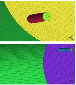
The model is meshed using unstructured hexahedron, and the boundary layer has been refined. The mesh consists of 125,600 nodes and 12, 0786 hexahedron elements, as shown in Figure 2. Mesh dependency had been tested before simulations.
2.3 Governing Equations
The continuity equation and Navier-Stokes equations provide a complete mathematical description of the velocity and pressure fields for any fluid dynamics problem [9, 10]. The continuity equation is given as follows:
( )
u( )
v( )
w 0t x y z
ρ ρ ρ
ρ ∂ ∂ ∂
∂ + + + =
∂ ∂ ∂ ∂
And the Navier-Stokes Equations are:
( ) ( ) ( ) ( )
( ) ( ) ( ) u
u uu uv uw
t x y z
u u u p S
x x y y z z x
ρ ρ ρ ρ
μ μ μ
∂ +∂ +∂ +∂
∂ ∂ ∂ ∂
∂ ∂ ∂ ∂ ∂ ∂ ∂
= + + − +
∂ ∂ ∂ ∂ ∂ ∂ ∂ (2)
( ) ( ) ( ) ( )
( ) ( ) ( ) v
v vu vv vw
t x y z
v v v p S
x x y y z z y
ρ ρ ρ ρ
μ μ μ
∂ ∂ ∂ ∂
+ + +
∂ ∂ ∂ ∂
∂ ∂ ∂ ∂ ∂ ∂ ∂
= + + − +
∂ ∂ ∂ ∂ ∂ ∂ ∂ (3)
( ) ( ) ( ) ( )
( ) ( ) ( ) w
w wu wv ww
t x y z
w w w p S
x x y y z z z
ρ ρ ρ ρ
μ μ μ
∂ +∂ +∂ +∂
∂ ∂ ∂ ∂
∂ ∂ ∂ ∂ ∂ ∂ ∂
= + + − +
∂ ∂ ∂ ∂ ∂ ∂ ∂ (4)
where x, y and z are the coordinates, u, v, w are the velocity components in x, y and z direction, respectively; P (Pa) is the pressure,ρ is the density and μ is the viscosity; Su, Sv, Sw are the source items
in x, y and z direction, respectively.
Generally, it is not possible to get analytical solutions to the Navier-Stokes equations except for some special cases, and numerical approaches have to be employed.
2) Temperature Equation
To conduct a detailed heat transfer analysis, the energy equation must also be considered, and this is shown as below:
( ) ( ) ( ) ( )
( ) ( ) ( ) T
p p p
T uT vT wT
t x y z
k T k T k T S
x c x y c y z c z
ρ ρ ρ ρ
∂ +∂ +∂ +∂
∂ ∂ ∂ ∂
∂ ∂ ∂ ∂ ∂ ∂
= + + +
∂ ∂ ∂ ∂ ∂ ∂ (5) where T (K) is the temperature, ρ(kg/m3), ν (m2/s), and κ (m2/s), c
p (J/Kg-K ) are the density, kinematic viscosity, thermal diffusivity, specific heat of fluid and ST is source item, respectively.
3) Turbulence Models
A number of studies have shown that significant turbulence can be found near the tank and inlet/outlet interface, even for the case of very low cold water charging rate. Currently, it is still beyond the capabilities of average computers to fully resolve the random and irregular details of a turbulent flow. However, the time averaged flow fields (both pressure and velocity) can be simulated reasonably accurately by the introduction of turbulence models.
the flow. This allows the models taking history effects such as convection and the diffusion of turbulent energy into consideration. The first is the transported turbulent kinetic energy (k) and it is a measure of the overall energy of the turbulence. The second is the turbulent energy dissipation (ε) which determines the scale of the turbulence. There are several types of k-ε models, but the Standard k-ε model and RNG k-ε
model are most popular. The RNG k-ε model is a modification of the standard model that attempts to account for different scales of motion. The RNG k-ε model used in this work .
4) Model and setting
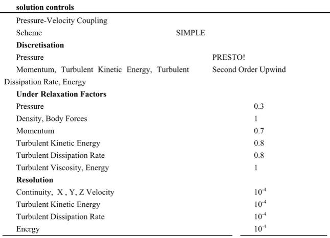
The first step for simulations is to define the solver and models to apply. For transient buoyancy driven flows, a pressure based solver with the energy equation model activated is considered appropriately. As the main focus is to be on a transient solution, time is selected to be unsteady. Also, the 2nd order implicit time formulation is selected rather than the first order as it improves the accuracy of the solution. All other inputs are left as the standards. The solver parameters that we are used are summarized in Tables1 [11], the fluid properties used in the model are presented in Tables 2, the operating conditions and boundary conditions are listed in Tables 3 and 4, respectively, and the solution controls are summarized in Table 5.
Table 1 Solver controls
Solver Controls
Solver Pressure Based
Space 3D Time Unsteady, 2nd-Order Implicit Viscous RNG k-epsilon turbulence model Energy Equation Yes
Table 2 fluid properties at 315K
Liquid Water Properties
Density (Boussinesq) 990.9 kg/m3
Specific Heat (Constant) 4180 J/Kg-K
Thermal Conductivity (Constant) 0.6 W/m-K
Viscosity (Constant) 0.001003 Kg/m-s
Thermal Expansion Coefficient (Constant) 0.00021 K-1
Table 3 operating conditions
Operating Conditions
Operating Pressure (KPa) 101.325
Gravity in the X direction (m/s2) 0
Gravity in the Y direction (m/s2) -9.81
Gravity in the Z direction (m/s2) 0
Boussinesq Operating Temperature (K) 315
Table 4 oundary conditions
Boundary Conditions
Inlet Velocity Magnitude (m/s) 0.25, 0.5, 1
Inlet Temperature (k) 293
Outlet Pressure outlet
Table 5 solution controls
solution controls Pressure-Velocity Coupling
Scheme SIMPLE Discretisation
Pressure PRESTO! Momentum, Turbulent Kinetic Energy, Turbulent
Dissipation Rate, Energy
Second Order Upwind
Under Relaxation Factors
Pressure 0.3
Density, Body Forces 1
Momentum 0.7
Turbulent Kinetic Energy 0.8
Turbulent Dissipation Rate 0.8
Turbulent Viscosity, Energy 1
Resolution
Continuity, X , Y, Z Velocity Turbulent Kinetic Energy Turbulent Dissipation Rate Energy
10-4
10-4
10-4
10-4
3. Results and Analysis
3.1 Evolution of transient temperature contours
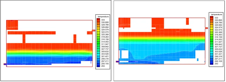
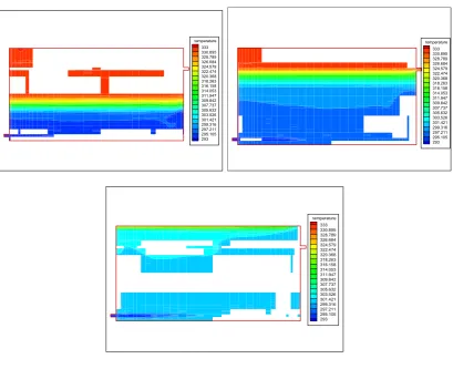
The simulations are conducted under the case with continuous hot water withdrawal, and the simulations are ended as the outlet water temperature is lower than 305K. After the simulations are completed, several typical sections of the tank are taken to show the interior flow patterns and temperature contours for each meshed geometry. In this work, temperature contours on the central section (z=0) are presented for analysis. The isothermal on the central section of the tank (z=0) for different inlet velocity (0.25m/s, 0.5m/s, 1m/s) at different times (10 min, 20 min, 30 min ) are presented in Figures 3 - 5.
It can be seen from Figures 3-5 that the inlet velocity has a significant influence on the thermal stratification inside the tank, and an increase in the inlet velocity will lead to stronger water mixing in the tank; when the inlet velocity is low, the thermal energy contained in the water layer above the outlet level is hard to be removed; when the inlet velocity is high, the water above the outlet level will mix with the water below the outlet level and therefore the thermal energy in the water layer above the outlet level can be removed. Hence, the outlet place in the tank is important for the removal of useful energy as the inlet velocity is not high.
3.2 Water mixing in the tank
(
)
( )
capture i a i
T T
T T
α= − −
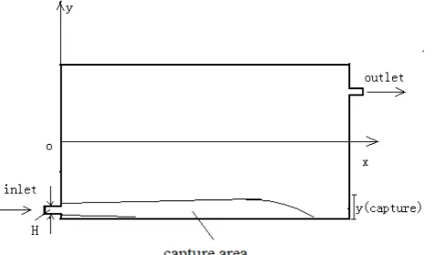
[image:6.544.150.377.177.288.2](6) where Ti is the inlet cold water temperature, Ta is the initial hot water temperature in the tank ,ycapture is the height of capture area and Tcapture is the average temperature over the capture area where z=0 and ycapture height. The capture area is the area where the flow velocity is equal to or greater than 0, as shown in Figure 6. Results of entrainment factors are listed in Table 6, where the ‘/’ represents the cases of the outlet temperature less 305K and simulation ended.
Table 6 The entrainment factor for different velocity (Ti=293K, Ta=333K)
a vi=0.25m/s vi=0.5m/s vi=1m/s
10 min 0.1325 0.2582 0.3046
20 min 0.0350 0.1385 0.2074
30 min 0.0326 0.0843 0.2038
40 min 0.0276 0.0580 /
50 min 0.0254 / /
60 min 0.0213 / /
70 min 0.0184 / /
80 min 0.0157 / /
3.3 The useful energy removed from the tank
5) Water discharging curves
Water discharging curves for different inlet velocities are presented in Figure 7. It is found that the temperature of the water discharged from the tank undergoes three stages: stable high-temperature stage, rapid decrease stage and stable low temperature stage, and the time durations these stages are all related to the inlet velocity.
6) Useful energy removal from the tank:
The maximum useful energy removed from the tank, Qu, can be obtained by: )
( s e
p
u mc T T
Q = − (7)
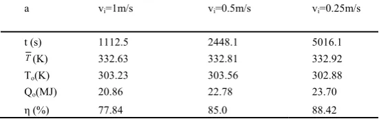
where m is the water mass in the tank, Ts is the initial hot water temperature in the tank and Te is the terminal water temperature in the tank. Given Ts= 333K and Te=305K, the maximum heat removal from the tank should be 26.8MJ, and the actual value can be calculated by summing useful heat removal at any moment over the period of water discharging period based on the water discharging curves. The heat removal efficiency η is the actual Qu divided by the maximum Qu and given in Table VII. It shows that the heat removal efficiency decreases with the increase in inlet velocity.
Table 7 The useful energy removed from the tank under various operation conditions (Ti=293K)
a vi=1m/s vi=0.5m/s vi=0.25m/s
t (s) 1112.5 2448.1 5016.1
T(K) 332.63 332.81 332.92
To(K) 303.23 303.56 302.88
Qo(MJ) 20.86 22.78 23.70
[image:6.544.125.401.544.631.2]4. Conclusions
Results obtained in this work indicate that increasing the inlet velocity will result in a larger entrainment factor and stronger water mixing in the tank; when the inlet velocity is not high, the thermal energy in the water layer above the outlet level is hard to be removed, whereas when the inlet velocity is too large, the water above the outlet level will mix with the water below the outlet level and therefore the thermal energy in the water above the outlet level can be removed but will cause stronger water mixing in the tank.
The temperature of water discharged from tank undergoes three stages: stable high-temperature stage, rapid decrease stage and stable low-temperature stage, and the time durations for these stages are related to the inlet velocity. With the increase in inlet velocity, the heat discharging efficiency decreases and the mixing of hot water in the tank and the supplied cold water becomes more significant.
5. Acknowledgment
The financial support by the National Natural Science Foundation of China (50879074, 11072211), Yunnan Science Foundation (2005E0021Q) and the Program for Changjiang Scholars and Innovative Research Team in University of Ministry of Education of China is gratefully acknowledged.
References
[1] Garg HP, Mullick SC, Bhargava AK. Solar thermal energy storage. Dordrecht: D.Reidel Publishing Company, 1985. [2] Furbo S, Andersen E, Thur A, Shah LJ, Andersen KD. Performance improvement by discharge from different levels in solar storage tanks. Solar Energy 2005, 79:431–9.
[3] Hegazy AA, Diab MR. Performance of an improved design for storage-type domestic electrical water-heaters. Applied Energy 2002, 71: 287–306.
[4] Hegazy AA. Effect of inlet design on the performance of storage-type domestic electrical water heaters. Applied Energy 2007, 84:1338–55.
[5] Lin W, Lu E. Parametric studies of thermosyphon solar water systems with electric heaters. Energy 1992, 7:397–403. [6] Lin W, Lu E. Analyzing the effect of the LAEH in the storage tank on the performance of a TSAEH. Int J Energy Res 1992, 16:459–66.
[7] Perez IR. Unsteady laminar convection in cylindrical domains: numerical studies and application to solar water storage tanks, Ph.D. Thesis. Barcelona: UPC – Barcelona Tech; 2006.
[8] Ievers S, Lin W. Three dimensional flow dynamics in a hot water storage tank, B. Eng. Thesis. Townsville, Australia: School of Engineering, James Cook University;2008.
[9] MUNSON, B. R., D. F. YOUNG, et al. (2002). Fundamentals of Fluid Mechanics. Hoboken, NJ, John Wiley & Sons. [10] John D. Anderson, JR. Computational Fluid Dynamics[M]. McGraw-Hill Companies,Inc.,1995.
[11] ANSYS. Fluent. <http://www.Fluent.com/.2008>.
Figure 1 Physical model of the studied hot water storage tanks and the coordinate system employed in this work.
[image:8.544.113.377.262.560.2]temperature 333 330.895 328.789 326.684 324.579 322.474 320.368 318.263 316.158 314.053 311.947 309.842 307.737 305.632 303.526 301.421 299.316 297.211 295.105 293
Figure 4 The temperature contours for different inlet velocities (0.25m/s, 0.5m/s, 1m/s) at time of 20 min
temperature 333 330.895 328.789 326.684 324.579 322.474 320.368 318.263 316.158 314.053 311.947 309.842 307.737 305.632 303.526 301.421 299.316 297.211 295.105 293 temperature 333 330.895 328.789 326.684 324.579 322.474 320.368 318.263 316.158 314.053 311.947 309.842 307.737 305.632 303.526 301.421 299.316 297.211 295.105 293 temperature 333 330.895 328.789 326.684 324.579 322.474 320.368 318.263 316.158 314.053 311.947 309.842 307.737 305.632 303.526 301.421 299.316 297.211 295.105 293
[image:10.544.45.455.256.589.2]Figure 6 Schematic of the capture area.