Coupled simulation-optimization model for coastal aquifer management using genetic programming-based ensemble surrogate models and multiple-realization optimization

Coupled simulation-optimization model for coastal aquifer

management using genetic programming-based ensemble surrogate

models and multiple-realization optimization

J. Sreekanth1,2_{and Bithin Datta}1,2

Received 21 June 2010; revised 9 November 2010; accepted 1 February 2011; published 29 April 2011.

[1] Approximation surrogates are used to substitute the numerical simulation model within

optimization algorithms in order to reduce the computational burden on the coupled optimization methodology. Practical utility of the surrogate-based simulation-optimization have been limited mainly due to the uncertainty in surrogate model simulations. We develop a surrogate-based coupled simulation-optimization methodology for deriving optimal extraction strategies for coastal aquifer management considering the predictive uncertainty of the surrogate model. Optimization models considering two conflicting

objectives are solved using a multiobjective genetic algorithm. Objectives of maximizing the pumping from production wells and minimizing the barrier well pumping for hydraulic control of saltwater intrusion are considered. Density-dependent flow and transport simulation model FEMWATER is used to generate input-output patterns of groundwater extraction rates and resulting salinity levels. The nonparametric bootstrap method is used to generate different realizations of this data set. These realizations are used to train different surrogate models using genetic programming for predicting the salinity intrusion in coastal aquifers. The predictive uncertainty of these surrogate models is quantified and ensemble of surrogate models is used in the multiple-realization optimization model to derive the optimal extraction strategies. The multiple realizations refer to the salinity predictions using different surrogate models in the ensemble. Optimal solutions are obtained for different reliability levels of the surrogate models. The solutions are compared against the solutions obtained using a chance-constrained optimization formulation and single-surrogate-based model. The ensemble-based approach is found to provide reliable solutions for coastal aquifer

management while retaining the advantage of surrogate models in reducing computational burden.

Citation: Sreekanth, J., and B. Datta (2011), Coupled simulation-optimization model for coastal aquifer management using genetic programming-based ensemble surrogate models and multiple-realization optimization,Water Resour. Res., 47, W04516, doi:10.1029/ 2010WR009683.

1. Introduction

[2] Coupled simulation-optimization models are

increas-ingly used as decision models to find optimal solutions to groundwater management problems like optimal ground-water remediation design, optimal extraction of groundground-water from coastal aquifers, and wetland management [Gorelick, 1983; Gorelick et al., 1984; Ahlfeld and Heidari, 1994;

Hallaji and Yazicigil, 1996; Emch and Yeh, 1998; Wang and Zheng, 1998; Das and Datta, 1999a, 1999b, 2000;

Cheng et al., 2000; Mantoglou, 2003; Mantoglou et al., 2004; Katsifarakis and Petala, 2006; Ayvaz and Karahan, 2008;Datta et al.2009]. One of the major disadvantages of using the coupled simulation-optimization model is the huge

computational burden involved due to multiple calls of the simulation model by the optimization algorithm. Recent studies have used nontraditional optimization techniques for solving groundwater management problems. This includes genetic algorithm [Aly and Peralta, 1999; Cheng et al., 2000; Qahman et al., 2005; Bhattacharjya and Datta, 2005], evolutionary algorithm [Mantoglou et al., 2004], simulated annealing [Rao et al., 2004], and differential evolution [Karterakis et al., 2007]. Population-based opti-mization algorithms like genetic algorithms can be effec-tively used to solve optimization problems considering multiple objectives at a time in which the entire nondomi-nated front of solutions can be obtained in a single run of the optimization model. However, with the use of population-based optimization algorithms like genetic algorithm, sev-eral thousands of evaluations of the simulation model may be required before an optimal solution is obtained. One possible approach to reducing the computational burden is to substitute the simulation model using approximate surro-gate models for simulation. In spite of the wide use of surrogate models in coupled simulation-optimization

1_{School of Engineering and Physical Sciences, James Cook University,}

Townsville, Queensland, Australia.

2_{CRC for Contamination Assessment and Remediation of the}

Environ-ment, Mawson Lakes, South Australia, Australia.

approaches, they are rarely accepted as reliable models for simulating groundwater flow and transport, in practical applications. These models are most often disfavored because of the inherently uncertain nature of these ‘‘black box’’ models.

[3] Use of the surrogate models adds an uncertainty

component to the simulation-optimization framework. Pre-dictive uncertainty of the surrogate models may have am-biguous effects on the optimality or even the feasibility of the obtained solutions. In the present study, we develop a coupled simulation-optimization model based on an ensem-ble of surrogate models for optimal management of coastal aquifers under the predictive uncertainty of the surrogate models. The model determines optimal extraction strategies for management. The ensemble of surrogate models is uti-lized to quantify the predictive uncertainty. The ensemble is then used with stochastic-optimization models to derive optimal extraction strategies.

[4] Previously, a number of different approaches have

been used to solve the problem of optimal and sustainable extraction of groundwater from coastal aquifers. The differ-ent approaches use either sharp interface or diffuse inter-face modeling of saltwater intrusion processes within a simulation-optimization framework. Analytical solutions exist for the sharp interface modeling approach and are comparatively easy to use in a simulation-optimization framework [Iribar et al., 1997;Dagan and Zeitoun, 1998;

Mantoglou, 2003; Park and Aral 2004; Mantoglou and Papantoniou, 2008]. The diffuse modeling approach con-siders the flow and transport equations which are linked together by the density dependence and needs to be simul-taneously solved. The coupled flow and transport equations are highly nonlinear and complex. Linking a numerical model which solves these equations with an optimization algorithm involves huge computational burden [Das and Datta, 1999a, 1999b;Dhar and Datta, 2009].

[5] In the past few years surrogate models have been

used as substitutes for the numerical simulation model within the optimization algorithm. A wide range of approx-imation surrogates have been used in different studies. Arti-ficial Neural Networks (ANN) have been widely used as approximation surrogates for groundwater models [ Ranji-than et al., 1993; Rogers et al., 1995; Aly and Peralta, 1999]. Neural network-based approximation surrogates were developed by Bhattacharjya and Datta[2005, 2009],

Yan and Minsker[2006],Kourakos and Mantoglou[2009], andDhar and Datta[2009] for use in simulation-optimiza-tion models. McPhee and Yeh[2006] used ordinary differ-ential equation surrogates to replace the partial differdiffer-ential equations of groundwater flow and transport.

[6] Most of these surrogate modeling approaches assume

a fixed surrogate model structure and optimize the surro-gate model parameters to obtain the best fit between the ex-planatory and response variables. Even the most popularly used neural network surrogate modeling approach deter-mines the optimal model architecture by trial and error [Bhattacharjya and Datta, 2005;Rao et al., 2004].

[7] In spite of the method used, developing surrogate

models from numerical simulation models results in a cer-tain amount of uncercer-tainty in the predicted variable. This is due to the uncertainty in the structure and parameters of the surrogate model. When used in a coupled

simulation-optimization framework to derive optimal groundwater management strategies, the uncertainties in the surrogate model predictions affect the optimality of the resulting solution. Thus, while achieving computational efficiency, increased mathematical uncertainty resulting from the residuals is introduced into the simulation-optimization framework by the surrogate model. Depending on the amount of uncertainty, the derived optimal solution may be rendered suboptimal or even infeasible. Hence, it is impor-tant to quantify the uncertainty in the surrogate model pre-dictions and reformulate the optimization problem to address this uncertainty.

[8] In our study, an ensemble-based surrogate modeling

approach based on genetic programming is used to predict the salinity intrusion into coastal aquifers resulting from groundwater extraction. Genetic programming (GP) has been used in hydrological applications in a few recent stud-ies [Dorado et al., 2002; Makkeasorn et al., 2008; Para-suraman and Elshorbagy, 2008; Wang et al., 2009]. GP has been used to develop prediction models for runoff, river stage and real-time wave forecasting [Babovic and Keijzer, 2002; Sheta and Mahmoud, 2001; Gaur and Deo, 2008].

Zechman et al. [2005] developed a GP-based surrogate model for use in a groundwater pollutant source identifica-tion problem. An ensemble-based GP framework is able to quantify the uncertainty in both the model structure and pa-rameters. Parasuraman and Elshorbagy [2008] illustrated the use of ensemble-based genetic programming frame-work in the quantification of uncertainty in hydrological prediction. Sreekanth and Datta [2010] used genetic pro-gramming to develop surrogate models for coastal aquifer management and compared it with modular neural net-work-based surrogate models. Genetic programming-based surrogate models have the advantage that the surrogate model structure need not be fixed prior to the model devel-opment. Instead, the optimum model structure is evolved by the self-organizing ability of genetic programming algo-rithm. It was found that GP-based surrogate modeling can develop simpler and effective surrogate models with model parameters as few as 30 against 1155 weights used in the neural network model. Also, it was demonstrated that the evolution of surrogate model structures by GP and its parsi-mony in identifying the input variables makes it more effective than the ANN model structure determined by trial and error and arbitrary selection of variables. In the present work we make use of GP to develop an ensemble of surro-gate models which are different from each other and use it for more reliable predictions of coastal aquifer processes for use in management model.

[9] Different stochastic optimization techniques have

coupled simulation-optimization model for groundwater remediation design under parameter uncertainty of the proxy simulators. The proxy simulators were based on a stepwise response surface analysis. The residuals in the prediction were treated as stochastic variables and their deterministic equivalent was incorporated into the optimization model.

[10] Most of the real world groundwater management

problems are multiobjective in nature, i.e., they involve more than one objective which are conflicting to each other. The solution to such problems is an entire nondomi-nated front of solutions which gives a trade-off between the different objectives considered. Population-based nontradi-tional optimization algorithms like genetic algorithms are ideal to solve such problems as different members of the population can converge to different parts of the nondomi-nated front, thus deriving the entire Pareto-optimal front in a single run of the optimization algorithm. Multiobjective genetic algorithm NSGA-II [Deb, 2001] is used in this study to solve the multiobjective optimal coastal aquifer management problem.

[11] In this work our main objective is to develop an

en-semble of surrogate models for predicting the saltwater intrusion process in coastal aquifers. The ensemble of sur-rogate models is used in a stochastic multiobjective opti-mization using multiple-realization approach to derive robust optimal extraction strategies which are less sensi-tive to the uncertainties in the surrogate model predictions. This study considers the uncertainties of the surrogate models alone and the numerical model is assumed to be certain. Two objectives of management are considered subject to the constraint of controlling saltwater intrusion. The first objective is to maximize the total pumping from the production wells tapping the aquifer. The second objective is to minimize the total pumping from a set of barrier wells which are used to hydraulically control salt-water intrusion. The salinity levels resulting from pumping is simulated using the surrogate simulation model. A chance-constrained optimization model is also developed for coastal aquifer management, taking into consideration the cumulative distribution function of the error residuals of surrogate model predictions. The optimal solutions obtained using these two methods is compared with the so-lution obtained using only a single-surrogate model in the coupled simulation-optimization model.

[12] The remaining part of this paper is structured as

follows. Section 2 describes the framework of the coastal aquifer management model. Section 3 describes the devel-opment of the ensemble of surrogate models. Section 4 describes the formulation and implementation of optimiza-tion models using multiobjective genetic algorithms. Sec-tion 5 illustrates the applicaSec-tion of the methodology using a case study. Section 6 summarizes and concludes the paper.

2. Outline of the Coastal Aquifer Management Methodology

[13] The proposed coastal aquifer management

method-ology using coupled simulation optimization has essentially two components. The first one is the ensemble of surrogate models for simulating the physical process under considera-tion. In this work we consider the saltwater intrusion in coastal aquifers as a function of the groundwater extractions

from the aquifer. The second component is an optimization model used to optimize the groundwater extraction strat-egies such that the resulting salinity levels are maintained within prespecified limits. The genetic programming-based surrogate models are trained using randomly generated input-output patterns of extraction rates and resulting salin-ity levels. The input-output patterns are generated using a three-dimensional simulation model for simulating coupled flow and transport called FEMWATER [Lin et al., 1997]. Nonparametric bootstrap method [Efron and Tibshirani, 1993] is used together with genetic programming to con-struct the ensemble of surrogate models. The ensemble models are then linked to a multiobjective genetic algorithm to obtain the optimal groundwater extraction rates. The dif-ferent elements of the proposed methodology for develop-ing optimal coastal aquifer management strategies are described in detail in sections 3 and 4.

3. Ensemble of Surrogate Models

[14] The following procedure was adopted to develop

the ensemble of surrogate models. 3.1. Design of Experiments

[15] The design of experiments is the first step required

for training the GP-based surrogate models. Developing a surrogate model based on genetic programming involves learning from input-output patterns. In the case of the coastal aquifer management problem, the inputs are the rates of groundwater abstractions from different potential locations within the aquifer and outputs are the resulting sa-linity concentrations. The decision space for the problem under consideration is a multidimensional space represent-ing the combinations of groundwater abstraction rates from different locations at various time periods. For the surro-gate models to perform satisfactorily, the training patterns should be representative of the entire decision space. Uni-formly distributed Latin hypercube samples (LHS) of input patterns are generated from the decision space to train the genetic programming-based surrogate models.

[16] LHS, a stratified-random procedure, provides an

ef-ficient way of sampling variables from their distributions [Iman and Conover, 1982]. The LHS involves samplingns

values from the prescribed distribution of each ofk varia-bles X1, X2,. . ., Xk. The cumulative distribution for each variable is divided intoNequiprobable intervals. A value is selected randomly from each interval The N values obtained for each variable are paired randomly with the other variables.

3.2. Numerical Simulation Model

[17] Once the input patterns of groundwater abstractions

are generated, the resulting salinity levels corresponding to each pattern are computed. The numerical simulation model FEMWATER [Lin et al., 1997] is used for this. FEM-WATER is a finite element-based 3-D coupled flow and transport simulation model. The density dependent flow and transport equations used in FEMWATER are given as fol-lows [Lin et al., 1997;Sreekanth and Datta2010]:

oF

@h

@t¼ r K rhþ orz

þ oq

F¼0

nþ

0_þndS

dh; ð2Þ

K¼g k¼

=_o

=o

og

o kskr¼

=o

=_oKsokr; ð3Þ

o¼a1þa2C; ð4Þ

@C @tþb

@Sa

@t þV rC r ðD rCÞ

¼ 0@h @tþ

CþbSa

ð Þ ðKwCþbKsSaÞ

þm qCþ F

@h

@tþ

o

V r _o @ @t C

ð5Þ

D¼aTjVjþðaLaTÞVV

jVjþam d; ð6Þ whereFis storage coefficient,his pressure head,tis time, Kis hydraulic conductivity tensor, zis potential head,qis source and/or sink,is water density at the chemical con-centration C,_o is referenced water density at zero chemi-cal concentration,is density of either the injection fluid or the withdrawn water, is moisture content,0is modi-fied compressibility of water, nis porosity of the medium,

Sis saturation,is dynamic viscosity of water at chemical concentration C, _o is referenced dynamic viscosity of water at zero chemical concentration, kis permeability ten-sor,ksis relative permeability or relative hydraulic

conduc-tivity, Kso is referenced saturated hydraulic conductivity

tensor,a1anda2are the parameters used to define concen-tration dependence of water density and Cis the chemical concentration, b is bulk density of medium,Cis material concentration in aqueous phase, Sa _{is material} concentra-tion in adsorbed phase, t is time, Vis discharge,r is del operator,Dis dispersion coefficient tensor,0is compressi-bility of the medium, his pressure head, is decay con-stant, m is qCin (artificial mass rate), q is source rate of water,Cinis material concentration in the source,Kwis first order biodegradation rate constant through dissolved phase,

Ksis first order biodegradation rate through adsorbed phase,

F is storage coefficient, jVj is magnitude ofV, dis

Kro-necker delta tensor, aTis lateral dispersivity,aLis longitu-dinal dispersivity,amis molecular diffusion coefficient, and

is tortuosity.

3.3. Genetic Programming

[18] Genetic programming [Koza, 1994] is used in this

study to evolve surrogate models for modeling the salinity intrusion in the coastal aquifers resulting from groundwater abstraction. Genetic programming is an evolutionary algo-rithm similar to genetic algoalgo-rithm in that it uses the concepts of natural selection and genetics in evolutionary computa-tion. For a given model structure and predefined parameter space, the genetic algorithm optimizes the parameter values. Genetic programming has an additional degree of freedom which allows an optimum model structure to evolve parallel

to optimizing the parameter values. Thus, genetic program-ming identifies the best model structure for simulating the process under consideration while simultaneously estimat-ing the optimal parameter values. Genetic programmestimat-ing learns from examples. The major inputs for the genetic pro-gramming model are (1) patterns for learning, (2) fitness function (e.g., minimizing the squared error term), (3) func-tional and terminal set, and (4) parameters for the genetic operators like the crossover and mutation probabilities.

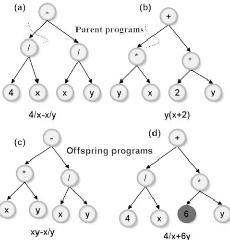
[19] The functional set consists of the basic

mathemati-cal operators and basic functions like addition, subtraction, multiplication, division, trigonometric functions, etc. The choice of the functional set determines the complexity of the model. For example, a functional set with only addition and subtraction results in a linear model structure, whereas a functional set which includes trigonometric functions result in highly nonlinear model structures. The terminal set consists of constants and variables of the model. The total number of parameters used can be limited to a prespe-cified number in order to prevent overfitting of the model. By using functional and terminal sets, valid syntactically correct programs can be developed. Parse tree notation of two such programs are illustrated in Figure 1. Two parent genetic programs are shown in Figures 1a and 1b. The par-ent programs are crossed over at the dashed sections and mutation operator changes the value of the constant 2 to 6 to generate two new offspring genetic programs shown in Figures 1c and 1d.

[20] In the present work, the operators addition,

subtrac-tion, and multiplication are considered in the initial func-tional set. Later, other functions were added into the functional set one by one in the order of their increasing complexity and nonlinearity. For example, an addition or subtraction operation is considered in the functional set before multiplication is considered. However, considering the nonlinear nature of the saltwater intrusion process, mul-tiplication and division are considered in the initial func-tional set itself. The addifunc-tional function or operator is accepted upon an improvement in the fitness measure because of this addition.

[21] GP starts with a set of randomly generated

syntacti-cally correct programs. Each program is evaluated by test-ing the programs inNnumber of instances, whereNis the number of patterns in the training data set generated using Latin hypercube sampling and the numerical simulation model. The input-output data set is split into halves. One half is used to train the GP models and the other half is used to test the developed genetic programs. Testing refers to the validation of the model. The testing data set is not used in the fitness function evaluation; instead it is used to evaluate how the model performs for a new set of data. Also, the evaluations based on the testing data set are used to pick the best programs from the population.

[22] By comparing the outcome of the program on each

3.4. Nonparametric Bootstrap Method

[23] The nonparametric bootstrap method is used to

gen-erate different realizations of the actual input-output patterns of groundwater abstractions and salinity concentrations. Each realization of the data set is then used to train a sepa-rate surrogate model. An ensemble of surrogate models for the prediction of salinity levels could be obtained using this procedure. Each surrogate model is distinctly different from the rest in the ensemble because of the difference in the training data set and the population based-optimization lead-ing to identification of multiple optima by the search algo-rithm. The distinction in the model structure and parameters among the different surrogate models is a manifestation of the uncertainty in the model structure and parameters itself. A methodology used by Parasuraman and Elshorbagy

[2008] is followed to accomplish nonparametric bootstrap sampling. The data set obtained using Latin hypercube sam-pling and using the numerical simulation model is assumed to be a representative set of input-output values from the entire population in the decision space. A training data setT

of sizeN is generated using Latin hypercube sampling and the numerical simulation model. Different realizations of this data set are obtained using the nonparametric bootstrap method. For this a bootstrap size ofBis chosen. ThenB dif-ferent data sets each of sizeNis obtained by repeated ran-dom sampling with replacement from the set T.Thus each bootstrap sample-set TB has different input-output patterns from the training data setTrepeated many times. The boot-strap sample setsTBdiffer from each other only in terms of the repetition of some patterns and elimination of some from the original data set. The repetition of patterns in the boot-strap causes differential weighting of these patterns. This results in development of the models which are different in their predictive capability in different regions of the decision space of the prediction model. This also triggers the conver-gence to multiple optimal solutions while training the

predic-tion model. Thus each surrogate model is an optimal model for the prediction, however different in their predictive capa-bility in different regions of the decision space, depending on the weights assigned to patterns from each region.

[24] The performance of each of the surrogate models is

determined by evaluating the root mean square error on the testing data set. After computing the root mean square errors for each of the surrogate model in the ensemble, the standard deviation and coefficient of variation of these errors are computed. The coefficient of variation of these errors is a measure of the predictive uncertainty of the models. The number of surrogate models in the ensemble is determined by performing an incremental statistical analysis on the en-semble performance, i.e., surrogate models are sequentially added in to the ensemble and the resulting uncertainty is evaluated. Also, the RMSE of the resulting ensemble is also computed after the addition of each surrogate model. RMSE is computed on the testing data considering the testing data sets of all the surrogates in the ensemble taken together at each stage of addition. The optimum number of surrogate models in the ensemble is determined as follows. An ensem-ble with 10 surrogate models is considered initially. The root mean square error of the salinity concentration predictions by each surrogate model is computed. The coefficient of var-iation of these root mean square errors are computed and is considered as the measure of uncertainty in the ensemble of models. Then, new surrogate models are added into the en-semble one at a time and the resulting RMSE and uncer-tainty are computed. This procedure is repeated until there is no significant change in the uncertainty of the ensemble with further addition of surrogate models. The number of surro-gate models in the ensemble at this stage is the ensemble size. The number of models in the ensemble at which further addition of models into the ensemble do not produce signifi-cant change in the uncertainty is considered as the optimum number of surrogate models in the ensemble.

4. Optimization Models

[25] The main objective of this study is to develop a

coastal aquifer management model which uses an ensemble of surrogate models to simulate the saltwater intrusion pro-cess. Two approaches of optimization addressing the uncer-tainty in surrogate model predictions are used in this study. The first one is based on a stochastic simulation-optimization method called multiple realization or stacking approach [Wagner and Gorelick, 1989; Morgan et al., 1993; Chan, 1993; Feyen and Gorelick, 2005]. The second approach uses a chance-constrained optimization model [Morgan et al., 1993;Datta and Dhiman, 1996].

[26] The stochastic optimization accounts for the

uncer-tainty in the surrogate model structures and parameters. In the multiple-realization approach all the surrogate models in the ensemble are independently linked to the optimiza-tion model, i.e., if the ensemble consists of 10 different sur-rogate models then the optimization formulation has a stack of 10 constraints representing the surrogate models. Thus the optimal solution will be subject to satisfying each of these constraints representing the different surrogate models which differ from each other due to the model structure and parameter uncertainty.

4.1. Multiobjective Optimization Using a Multiple-Realization Approach

[27] Two conflicting objectives are considered in this

study. The first one is the maximization of total beneficial pumping from the aquifer and the second one is minimiza-tion of the total pumping from the barrier wells which are used to hydraulically control saltwater intrusion. Limiting the salinity concentrations, resulting from the groundwater extraction, to specified limits are the constraints. The math-ematical formulation of this multiobjective optimization problem using multiple-realization approach is as follows:

Maximize; f1ðQÞ ¼ XN

n¼1 XT

t¼1 Qt

n; ð7Þ

Minimize; f2ðQÞ ¼ XM

m¼1 XT

t¼1 qt

m; ð8Þ

s:t:cr i ¼

r

iðQ;qÞ 8i;r; ð9Þ

cr

i cmax8i;r; ð10Þ

QminQtnQmax ð11Þ

qminqtmqmax; ð12Þ

whereQt

nis the pumping from thenth production well dur-ing thetth time period,qt

mis the pumping from themth bar-rier well during the tth time period, and cr

i is the rth

realization of concentration in the ith location at the end of the management time horizon. This is obtained from therth surrogate model for the salinity at the ith location using the surrogate model given by _ir( ).M, N, and T are, respec-tively, the total number of production wells, total number of barrier wells, and total number of time steps in the

man-agement model. Constraint (10) imposes the maximum per-missible salt concentration in the monitoring well locations. Constraints (11) and (12) define lower and upper bounds of the pumping from production wells and barrier wells, respectively.

[28] With the multiple-realization approach, optimal

sol-utions with different reliability values can be obtained. The reliability value is the fraction of surrogate models in the entire ensemble whose salinity predictions satisfy the imposed constraints of maximum salinity levels in the optimization model. For example, if there are N different surrogate models in the ensemble, it is possible to obtain an optimal solution with a reliability of n=_N by constraining the optimization model to satisfy constraints imposed by at leastnsurrogate models. Reliability of the optimal solu-tion is close to 1 when the constraints imposed by all N

surrogate models are satisfied. However, this reliability per-tains to the uncertainty in the ensemble of surrogate models only.

4.2. Chance-Constrained Approach

[29] The optimal solutions obtained by the

multiple-realization approach for different reliabilities are compared to the solutions obtained using a chance-constrained opti-mization formulation. The chance-constrained formulation uses the same objective functions and constraints as in (7) and (8) and (11) and (12). The constraint given by (10) and (11) are replaced as follows:

ci¼iðQ;qÞ þ"i; ð13Þ

Rel½ciðQ;q; "iÞ cmax ; ð14Þ where ci is the salinity concentration at the ith location at the end of the management time horizon, "i is the error in the salinity concentration prediction for the ith location, and_iðQ;qÞis the average of the salinities at the ith loca-tion predicted by the ensemble of surrogate models. Rel is the reliability level of the ensemble prediction that the pre-dicted concentration is less than cmax. This reliability is based on the cumulative distribution function of the error residuals in the salinity level prediction by the surrogate models. The reliability is constrained to be greater than or equal to. The probabilistic constraint in (14) is converted into its deterministic equivalent as follows:

_iðQ;q; "iÞ þi1ð Þ cmax; ð15Þ where i1 is the inverse cumulative distribution function for the residuals in salinity prediction at the ith location and i1ð Þ gives the prediction error corresponding to a reliability.

[30] A coupled simulation-optimization model with a

single-surrogate model predicting the salinity levels at each monitoring location is also developed for comparative eval-uation. The same optimization formulation as in (7) – (12) is used for this purpose except that salinity prediction by the ensemble represented by (9) is replaced as follows:

where_ib represents the best surrogate model, in terms of the least value of the objective function obtained in the GP model, for predicting the salinity at the ith location. The original data set is used to develop this surrogate model instead of the bootstrap sample.

4.3. Multiobjective Genetic Algorithm

[31] A multiobjective genetic algorithm NSGA-II [Deb,

2001] is used to solve the multiobjective coastal aquifer management problem. Similar to GA, NSGA-II uses a pop-ulation of candidate solutions together with the GA opera-tors cross-over, mutation and selection to evolve improves solutions to the optimization problem over a number of generations. In addition to this, NSGA-II organizes the members of the population into nondominated fronts after each generation, based on the conflicting objectives of opti-mization. Thus, in a single run, NSGA-II is able to generate the entire Pareto-optimal set of solutions at the end of the specified number of generations.

4.4. Ensemble-Based Coupled Simulation-Optimization Model

[32] The coastal aquifer management model makes use

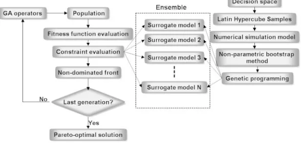
of a coupled simulation-optimization framework to derive the optimal groundwater extraction strategies for coastal aquifers. The ensembles of the surrogate model for simulat-ing the aquifer responses in terms of salinity concentrations are coupled with the optimization model by linking each surrogate model separately with the optimization algorithm. The multiobjective genetic algorithm randomly generates candidate solutions which are the groundwater extraction rates for the different time periods within the management horizon. The aquifer responses corresponding to each of these patterns of extraction are obtained from the ensemble of surrogate models. All generated candidate solutions are evaluated for feasibility and fitness. New candidate solu-tions are generated using the genetic algorithm operators. The procedure is repeated for a number of generations, until the termination criteria are satisfied. The solutions are pro-gressively improved to converge to the final Pareto-optimal front. A schematic representation of the ensemble-based simulation-optimization model is shown in Figure 2. 4.5. Validation

[33] Once the optimal solution is obtained, its validity is

checked by simulating the aquifer processes by using the

optimal pumping values in the actual numerical simulation model FEMWATER. The residual in the salinity predic-tion, i.e., the difference between the surrogate-predicted value and the numerically simulated value, is evaluated for five optimal solutions in different regions of the Pareto-optimal front. This is performed for the Pareto-optimal solutions obtained using the three optimization models, namely, single-surrogate model, ensemble-based model, and the chance-constrained model.

5. Case Study

[34] In order to illustrate the application of the proposed

methodology, it is applied to derive optimal extraction strategies for an illustrative coastal aquifer system. The aq-uifer is 2.52 km2_{in aerial extent with eight potential} loca-tions for groundwater extraction for beneficial use, and three potential barrier well locations for hydraulic control of salinity intrusion. The aquifer considered is single lay-ered with an average depth of 60 m. The boundaries of the study area are all no-flow boundaries, except for the sea-ward side boundary which is a constant head and constant concentration boundary with a concentration value of 35 kg/m3_{. The aquifer system is illustrated in Figure 3. The} eight potential locations for beneficial groundwater extrac-tion are shown as PW1 – PW8. The barrier well locaextrac-tions for hydraulic control of saltwater intrusion are shown as BW1 – BW3. The salinity concentrations were monitored at three locations, C1, C2, and C3, at the end of the manage-ment time horizon.

[35] The time horizon for the management model was

fixed as 3 years with the extraction rates in each manage-ment period of 1 year considered as uniform. The ground-water recharge is specified as a constant rate of 0.00054 m/d, respectively. The lower and upper limits on groundwater abstractions for both beneficial and barrier wells are 0 and 1300 m3_{/d. Total number of decision variables in the} optimi-zation model is 33, corresponding to pumping from 11 wells for three time periods. The management model specifies a maximum permissible salt concentration limit of 0.5, 0.6, and 0.6 kg/m3_{at these locations, respectively. The} parame-ters used for the FEMWATER model are given in Table 1.

[36] A three-dimensional coupled flow and transport

simulation model was used to simulate the aquifer pro-cesses resulting in salinity intrusion due to groundwater

abstraction in this study area. Different groundwater extrac-tion scenarios were generated using Latin hypercube sam-pling. The salinity concentrations resulting from each of these pumping patterns are simulated using FEMWATER. The simulated salinity level and the corresponding pump-ing rates form the input-output pattern. Altogether 230 extraction patterns are used in this study. Different realiza-tions of this input-output data set were generated using the nonparametric bootstrap method. Each of these data sets was used to build surrogate models to create the ensemble of surrogate models. Each data set was split into halves for training and testing the GP models. The input-output pat-terns were then used to train the genetic programming-based surrogate models. Adaptive training [Sreekanth and Datta, 2010] was performed to reduce the number of pat-terns required for training.

[37] Surrogates were developed for predicting salinity at

three different locations. For each location 30 models in the ensemble was found to be sufficient to characterize the uncertainty. All the genetic programming surrogate models used a population size of 500, mutation frequency of 95, and crossover frequency of 50. A commercial genetic pro-gramming software Discipulus was used to develop the sur-rogate models. The parameters values, as per the guidelines after performing a sensitivity analysis, were used in the de-velopment of the model. The functional set in the developed GP models contained the operations addition, subtraction, multiplication, division, comparison, and data transfer. The maximum number of surrogate model parameters used was limited to 30 to prevent overfitting of the model. Squared deviation from the actual value was used as the fitness func-tion. At the end of model training and testing source codes

of the model in C language were generated using the inter-active evaluator of the software and are then coupled with the multiobjective optimization algorithm NSGA II.

6. Results and Discussion

6.1. Uncertainty in Surrogate Models

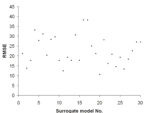
[38] The uncertainty in the surrogate models were

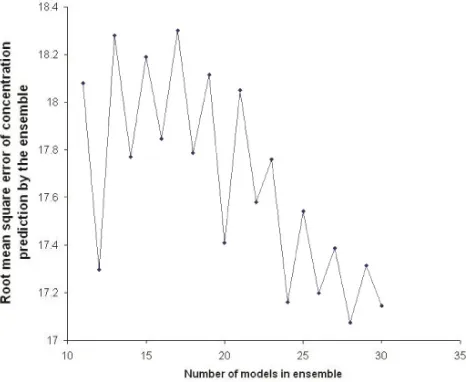
quanti-fied using the coefficient of variation of the root mean square errors of the individual surrogate models. The root mean square errors of individual surrogate model salinity predic-tions C1, C2, and C3 are shown in Figures 4, 5, and 6. The RMSEs are computed over the testing data set used for eval-uating the genetic programming-based surrogate models. It could be observed that for different realizations of the same data set, the root mean square errors are different for differ-ent surrogate models. This is due to the predictive uncer-tainty of the surrogate models. The root mean square errors for the ensemble of models predicting salinity C1 are plotted against the number of surrogate models in the ensemble starting from an initial ensemble size of 10 in Figure 7. As the number of models in the ensemble increases, RMSE of the ensemble prediction decreases, at least in this example.

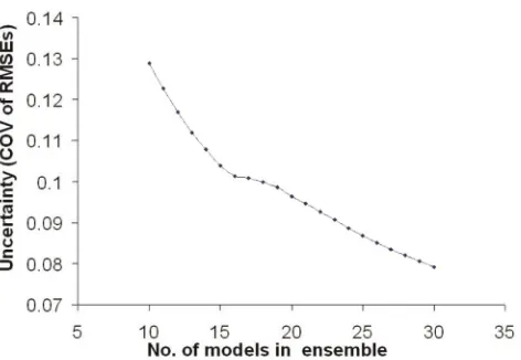
[39] The coefficient of variation of the RMSEs, as a

mea-sure of uncertainty in prediction of salinity, is plotted against the number of surrogate models in the ensemble for each ensemble predicting C1, C2, and C3. The plots are shown in Figures 8, 9, and 10. Uncertainty of the ensemble model has a definite decreasing trend with the increasing number of models in the ensemble. For each of the salinity concentrations C1, C2, and C3 the uncertainty in the en-semble of surrogate model decreases with the number of models in the ensemble and reaches a constant value when the number of models in the ensemble is around 30. Hence the optimum number of models in the ensemble for coupled simulation optimization is chosen as 30. The optimum number of surrogate models depends on the uncertainty level in the model structure and parameters. For more com-plex systems the uncertainty in the model structure and pa-rameters of surrogate models will be larger and hence more number of surrogate models will be required in the ensem-ble. The sensitivity of the derived Pareto-optimal solutions to the number of surrogate models in the ensemble is ana-lyzed in section 6.4.

Table 1. Parameters for Aquifer Simulation

Parameter Value

Hydraulic conductivity inxdirection 25 m/d Hydraulic conductivity inydirection 25 m/d Hydraulic conductivity inzdirection 0.25 m/d Longitudinal dispersivity 80 m/d

Lateral dispersivity 35 m/d

Molecular diffusion coefficient 0.69 m2_/d

Soil porosity 0.2

Density reference ratio 7.14107

Figure 5. RMSE for individual surrogate models simulating salinity C2. Figure 4. RMSE for individual surrogate models simulating salinity C1.

6.2. Multiobjective Optimization

[40] The multiobjective optimization algorithm NSGA-II

was used to solve the optimization formulations of both multiple-realization and chance-constrained approaches. Similar to an ordinary genetic algorithm, NSGA-II has a population-based approach for deriving the optimal solu-tions. The population size used in this study is 200. NSGA-II was run for 750 generations to obtain the optimal solution. Thus a total of 200750 evaluations of the aquifer response to specific groundwater extraction patterns would be required before obtaining the solutions. The NSGA-II pa-rameters used were crossover probability 0.9 and mutation probability 0.02. The sensitivity of the optimal solution to population size, number of generations, and NSGA-II pa-rameters were evaluated by conducting a number of numeri-cal experiments by running the NSGA-II model with different combinations of the parameters. It was found that for the number of generations less than 750 and population size less than 200, convergence to the Pareto-optimal front is not achieved. However, convergence is obtained for a smaller population size of a larger number of generations. It is noted that reducing the population size affects the spread of solutions in the Pareto-optimal front. Some regions of the Pareto-optimal front get eliminated as a result of reduction in the population size. The optimization problems have 33 variables which are the pumping rates from 11 locations for three time periods. The optimization by multiple-realization approach has 90 constraints, corresponding to three ensem-bles with 30 surrogate models each predicting the salinity levels C1, C2, and C3.

6.3. Pareto-Optimal Front

[41] Pareto-optimal solutions refer to a nondominated

front of solutions obtained for the coastal aquifer manage-ment problem. On the Pareto-optimal front any improve-ment in one objective function requires a corresponding decline in the other objective function. These sets of solutions are obtained for the coastal aquifer management problem using multiobjective optimization for both multiple-realization and chance-constrained approaches. All the solu-tions on the front are nondominated and the water managers

can choose a prescribed solution to implement a specific pumping pattern so as to maximize the benefits and simulta-neously limiting the aquifer contamination.

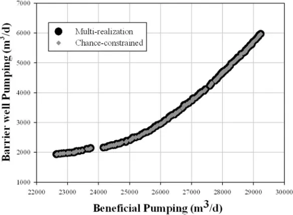
[42] The Pareto-optimal solutions for different reliabilities

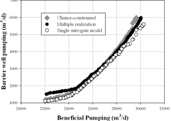
obtained by the multiple-realization and chance-constrained methods are compared in Figures 11– 13. Figure 11 illus-trates the Pareto-optimal front for a reliability of 0.99. In the multiple-realization approach this set of solutions satisfy the constraints imposed by all the surrogate models linked with the optimization model. In the chance-constrained formula-tion this set of soluformula-tions corresponds to an error in predicformula-tion corresponding to a reliability of 0.99. Similarly Figures 12, 13, and 14 illustrate the fronts corresponding to reliability levels of 0.8, 0.66, and 0.5. Figure 14 also compares the fronts of reliability level 0.5 to the Pareto-optimal front obtained using single-surrogate model in optimization.

[43] For the multiple-realization approach the reliability

refers to the percent of surrogate models in the ensemble, the imposed constraints of which are satisfied in the optimi-zation. For the chance-constrained method the reliability is obtained from the inverse cumulative distribution function of the residuals in the salinity prediction by the ensemble of surrogate models for salinities C1, C2, and C3. The cu-mulative distribution functions corresponding to C1, C2, and C3 are shown in Figures 15, 16, and 17. The errors are more or less symmetrically distributed with a probability of 0.5 for zero residual in all three cases.

[44] It can be noted that Pareto-optimal solutions with a

Figure 8. Uncertainty levels for increasing ensemble size for salinity C1.

Figure 9. Uncertainty levels for increasing ensemble size for salinity C2.

with the reliability, it could be deduced that the reliability level of the solutions obtained using a single-surrogate model linked with the optimization algorithm is less than 0.5. In using a single best surrogate model in the coupled simulation optimization it is assumed that the surrogate model prediction has a 0 residual, i.e., the surrogate model simulation is equiv-alent to the numerical model simulation. However, it can be observed from the cumulative distribution functions that the probability of zero residual is 0.5. Since most of the optimal solutions are limit state designs, i.e., optimal solution lying on the constraint bounds, the uncertainty in the surrogate model structure often causes the optimal solution to move into the infeasible region.

[45] Salinity levels corresponding to five different

opti-mal solutions in the Pareto-optiopti-mal front, obtained using the

best surrogate model in the coupled simulation-optimization model, are shown in Table 2. It could be observed that, in the optimal solutions, the salinity levels C1 and C3 con-verge to the permissible maximum concentration and hence the solutions are on the constraint boundaries. Hence, a small error in the surrogate model prediction can move these solutions into the infeasible zone. The salinity levels corresponding to these solutions is simulated using the actual simulation model and is compared with the values obtained using the surrogate model. It could be observed that some of the actual salinity levels obtained from the nu-merical simulation model violate the constraints, thus forc-ing the derived optimal solutions into the infeasible zone. The errors in the predicted salinity level for the optimal solutions are given in Tables 3 and 4. Tables 3 and 4 Figure 11. Pareto-optimal fronts with reliability 0.99.

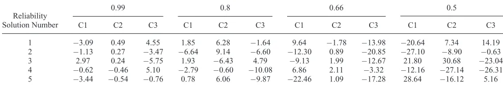
correspond to multiple-realization and chance-constrained approaches, respectively. The errors refer to the difference in the salinity levels obtained using the actual numerical simulation model and the surrogate model. In both the cases, it is evident that the errors are less when the reliabil-ity level is high.

[46] The ensemble-based surrogate modeling approach

quantifies the uncertainties in the model structure and pa-rameters. Reliable optimal solutions for coastal aquifer management were obtained using the ensemble surrogate models with the stochastic multiple-realization and chance-constrained optimization models.

6.4. Sensitivity Analysis

[47] Comparison of Pareto-optimal fronts for different

reliabilities show that for 30 surrogate models in the en-semble, the multiple-realization approach identifies the

same front as the chance-constrained optimization approach for identical reliability levels. This implies that the constraints imposed by stochastic optimization using multiple realization is as rigid as the chance constraints when the number of surrogate models in the ensemble is large enough to quantify the uncertainty in the model struc-tures and parameters.

[48] In order to investigate the effect of the number of

surrogate models in the ensemble, numerical experiments were performed with 15, 10, and 5 models in the ensemble for the multiple-realization optimization approach for each reliability level. The corresponding Pareto-optimal fronts for reliability level 0.99 are compared with the fronts obtained using 30 models and the chance-constrained model is shown in Figure 18. As the size of the ensemble decreases, the fronts move further to find seemingly better solutions, which actually may be infeasible solutions. Figure 13. Pareto-optimal fronts with reliability 0.66.

Figure 16. Cumulative distribution functions for the residuals in the ensemble predictions of salinity C2.

Table 2. Salinity Levels Corresponding to Five Optimal Solutions From Single-Surrogate Model-Based Optimizationa

Solution Number

C10.5 kg/m3 _{C20.6 kg/m}3 _{C30.6 kg/m}3

SM103_kg/m3 _NM103_kg/m3 _SM103_kg/m3 _NM103_kg/m3 _SM103_kg/m3 _NM103_kg/m3

1 500.00 483.04 563.39 561.45 599.99 622.05

2 500.00 515.33 583.13 575.97 599.99 623.52

3 500.00 510.34 582.39 573.16 599.99 599.76

4 500.00 483.00 574.68 548.73 599.99 624.23

5 500.00 498.25 574.48 563.57 599.99 618.35

a_{SM¼surrogate model, NM¼numerical model.}

Table 3. Residuals in Salinity Prediction for Five Optimal Solutions Obtained by Multiple-Realization Optimization

Reliability Solution Number

0.99 0.8 0.66 0.5

C1 C2 C3 C1 C2 C3 C1 C2 C3 C1 C2 C3

1 3.16 0.61 4.24 1.83 12.09 8.21 9.89 1.77 14.08 30.92 28.19 8.20 2 6.14 0.29 5.21 4.19 3.55 4.12 17.09 0.92 21.90 8.53 19.43 2.82 3 4.93 0.01 4.89 6.00 12.66 12.57 2.58 0.00 6.98 27.14 22.50 6.96 4 0.05 0.44 5.27 4.52 2.50 12.39 5.22 0.07 1.05 18.52 28.29 17.87 5 2.27 0.36 0.04 5.60 7.70 6.02 8.76 0.39 5.73 10.23 30.06 9.14

Table 4. Residuals in Salinity Prediction for Five Optimal Solutions Obtained by Chance-Constrained Optimization

Reliability Solution Number

0.99 0.8 0.66 0.5

C1 C2 C3 C1 C2 C3 C1 C2 C3 C1 C2 C3

1 3.09 0.49 4.55 1.85 6.28 1.64 9.64 1.78 13.98 20.64 7.34 14.19 2 1.13 0.27 3.47 6.64 9.14 6.60 12.30 0.89 20.85 27.10 8.90 0.63 3 2.97 0.24 5.75 1.93 6.43 4.79 9.13 1.99 12.67 21.80 30.68 23.04 4 0.62 0.46 5.10 2.79 0.60 10.08 6.86 2.11 3.32 12.16 27.14 26.31 5 3.44 0.54 0.76 0.78 6.06 9.87 22.46 1.09 17.28 28.64 16.12 5.16

Similar results were obtained for other reliability levels also. Hence, it can be inferred that the size of the ensemble has an effect on the stochastic optimization using multiple realizations. With a sufficiently large number of models in the ensemble, the multiple-realization approach performs similar to the chance-constrained optimization approach.

7. Summary and Conclusions

[49] Surrogate models are widely used in research to

sub-stitute complex numerical simulations models in solving groundwater management problems using coupled simula-tion-optimization. However, their practical applications have been limited primarily due to the reliability of the sur-rogate model predictions. The reliability of sursur-rogate model predictions is dependent on the uncertainties in the model structure and parameters. The uncertain surrogate models when used in a coupled simulation-optimization framework affects the quality as well as reliability of the optimal solu-tions obtained. Because most optimal design solusolu-tions are limit state in nature, the error in the surrogate model predic-tions could make the derived optimal solupredic-tions even infeasi-ble. In order to address these issues, and as a possible remedy, this study proposed and evaluated the performance of an ensemble of surrogate models based on a simulation-optimization model. The ensemble of surrogate models is also used to quantify the uncertainty in the surrogate model structure and parameters. Salinity prediction by each surro-gate model in the ensemble differs from others due to the model structure and parameter uncertainty. Two different optimization formulations were used to derive the optimal abstraction rates. In the first method, each surrogate model in the ensemble was independently linked to the multiobjec-tive genetic algorithm NSGA II, using the multiple-realiza-tion formulamultiple-realiza-tion. In the second method, the error in salinity predictions were quantified using the ensemble of models and the cumulative distribution function of the errors was obtained. Based on the cumulative distribution function, the chance-constrained optimization problem was formulated and solved using the multiobjective genetic algorithm NSGA II. The reliability of the chance-constrained model is analogous to the reliability obtained using the ensemble surrogate model approach, as the management model is strained by the permissible maximum limits on salinity con-centrations. The Pareto-optimal sets of solutions obtained using the two methods for different reliability levels were compared. Also, these fronts were compared with the Pareto-optimal set obtained using the best surrogate model in the coupled simulation optimization. It was observed that the front obtained using the single-surrogate model in the optimization was close to the front corresponding to a speci-fied reliability of 0.5. It could be argued that the reliability of the optimal solution obtained using a single-surrogate model in the linked simulation-optimization model for coastal aquifer management roughly corresponds to 0.5. However, using ensemble of surrogate models with stochas-tic optimization helps improve the reliability of the salinity predictions and subsequent optimal solutions.

[50] Ensemble-based surrogate modeling in

couple-simulation optimization has significant advantages over the single-surrogate modeling approach. The single-surrogate modeling approach does not take into consideration the

dictive uncertainty and assume that the surrogate model pre-diction is equivalent to numerical simulation. The ensemble-based methodology is able to quantify the predictive uncertainty and use it in a stochastic optimization model. Thus the ensemble-based approach accounts for the error in surrogate model prediction due to predictive uncertainty which is difficult to accomplish using the single-surrogate model. The ensemble-based approach is found to derive more reliable optimal solutions while retaining the computa-tional advantages of the surrogate modeling approach.

[51] It should be possible to use ensemble surrogate

mod-els in coupled simulation-optimization groundwater manage-ment studies considering the uncertainty in the groundwater parameters. Ensemble of surrogate models could be used to substitute groundwater models with different hydraulic con-ductivities and other uncertain parameters. For this, each member of the ensemble has to be trained using a different data set obtained by using a particular realization of the uncertain groundwater parameters in the numerical simula-tion model. The ensemble can be then used in a stochastic-optimization framework to derive groundwater management strategies under groundwater parameter uncertainty.

[52]Acknowledgments. This study was funded by CRC for Contami-nation Assessment and Remediation of the Environment, Australia. We are grateful to the four reviewers for the constructive comments which helped in improving the presentation of this paper.

References

Ahlfeld, D. P., and M. Heidari (1994), Applications of optimal hydraulic control to groundwater systems,J. Water Resour. Planning Manage., 120(3), 350 – 365.

Aly, A. H., and R. C. Peralta (1999), Optimal design of aquifer cleanup sys-tems under uncertainty using a neural network and a genetic algorithm, Water Resour. Res.,35(8), 2523 – 2532, doi:10.1029/98WR02368. Ayvaz, M. T., and H. Karahan (2008), A simulation/optimization model for

the identification of unknown groundwater well locations and pumping rates,J. Hydrol.,357(1 – 2), 76 – 92.

Babovic, V., and M. Keijzer (2002), Rainfall runoff modelling based on genetic programming,Nord. Hydrol.,33(5), 331 – 346.

Bhattacharjya, R., and B. Datta (2005), Optimal management of coastal aquifers using linked simulation optimization approach,Water Resour. Manage.,19(3), 295 – 320.

Bhattacharjya, R. K., and B. Datta (2009), ANN-GA-based model for mul-tiple objective management of coastal aquifers,J. Water Resour. Plan-ning Manage.,135(5), 314 – 322.

Chan, N. (1993), Robustness of the multiple realization method for stochas-tic hydraulic aquifer management, Water Resour. Res., 29(9), 3159 – 3167, doi:10.1029/93WR01410.

Cheng, A. H. D., D. Halhal, A. Naji, and D. Ouazar (2000), Pumping opti-mization in saltwater-intruded coastal aquifers, Water Resour. Res., 36(8), 2155 – 2165, doi:10.1029/2000WR900149.

Dagan, G., and D. G. Zeitoun (1998), Seawater-freshwater interface in a stratified aquifer of random permeability distribution, J. Contam. Hydrol.,29(3), 185 – 203.

Das, A., and B. Datta (1999a), Development of management models for sus-tainable use of coastal aquifers,J. Irrig. Drain. Eng. 125(3), 112– 121. Das, A., and B. Datta (1999b), Development of multiobjective management

models for coastal aquifers,J. Water Resour. Planning Manage.,125(2), 76 – 87.

Das, A., and B. Datta (2000), Optimization based solution of density depend-ent seawater intrusion in coastal aquifers,J. Hydrol. Eng.,5(1), 82–89. Datta, B., and S. D. Dhiman (1996), Chance constrained optical monitoring

network design for pollutants in groundwater,J. Water Resour. Planning Manage.,122(3), 180 – 189.

Dhar, A., and B. Datta (2009), Saltwater intrusion management of coastal aquifers. I: Linked simulation-optimization, J. Hydrol. Eng., 14(12), 1263– 1272.

Deb, K. (2001),Multi-objective Optimization Using Evolutionary Algo-rithms, John Wiley, New York.

Dorado, J., J. R. Rabunal, J. Puertas, A. Santos, and D. Rivero (2002), Pre-diction and modelling of the flow of a typical urban basin through genetic programming,Appl. Artifici. Intel.,17(4), 329 – 343.

Efron, B., and R. J. Tibshirani (1993),An Introduction to the Bootstrap, Monogr. on Stat. and Appl. Prob., vol. 57, Chapman and Hall, New York. Emch, P. G., and W. W. G. Yeh (1998), Management model for conjunctive use of coastal surface water and ground water,J. Water Resour. Planning Manage.,124(3), 129 – 139.

Feyen, L., and S. M. Gorelick (2005), Framework to evaluate the worth of hydraulic conductivity data for optimal groundwater resources manage-ment in ecologically sensitive areas,Water Resour. Res.,41, W03019, doi:10.1029/2003WR002901.

Gaur, S., and M. C. Deo (2008), Real-time wave forecasting using genetic programming,Ocean Eng.,35(11 – 12), 1166 – 1172.

Gorelick, S. M. (1983), A review of distributed parameter groundwater-management modeling methods,Water Resour. Res.,19(2), 305 – 319, doi:10.1029/WR019i002p00305.

Gorelick, S. M., C. I. Voss, P. E. Gill, W. Murray, M. A. Saunders, and M. H. Wright (1984), Aquifer reclamation design—The use of contami-nant transport simulation combined with non-linear programming,Water Resour. Res.,20(4), 415 – 427, doi:10.1029/WR020i004p00415. Hallaji, K., and H. Yazicigil (1996), Optimal management of a coastal

aqui-fer in southern Turkey,J. Water Resour. Planning Manage., 122(4), 233 – 244.

He, L., G. H. Huang, and H. W. Lu (2010), A coupled simulation-optimization approach for groundwater remediation design under uncertainty: An appli-cation to a petroleum-contaminated site, Environ. Pollution,157(8–9), 2485–2492.

Iman, R. L., and W. J. Conover (1982), A distribution-free approach to induc-ing rank correlation among input variables,Commun. Stat. B 11, 311–334. Iribar, V., J. Carrera, E. Custodio, and A. Medina (1997), Inverse modelling

of seawater intrusion in the Llobregat delta deep aquifer,J. Hydrol., 198(1 – 4), 226 – 244.

Karterakis, S. M., G. P. Karatzas, I. K. Nikolos, and M. P. Papadopoulou (2007), Application of linear programming and differential evolutionary optimization methodologies for the solution of coastal subsurface water management problems subject to environmental criteria, J. Hydrol., 342(3 – 4), 270 – 282.

Katsifarakis, K. L., and Z. Petala (2006), Combining genetic algorithms and boundary elements to optimize coastal aquifers’ management, J. Hydrol.,327(1 – 2), 200 – 207.

Kourakos, G., and A. Mantoglou (2009), Pumping optimization of coastal aquifers based on evolutionary algorithms and surrogate modular neural network models,Adv. Water Resour.,32(4), 507 – 521.

Koza, J. R. (1994), Genetic programming as a means for programming computers by natural-selection,Stat. Comput.,4(2), 87 – 112.

Lin, H.-C. J., D. R. Richards, C. A. Talbot, G.-T. Yeh, J.-R. Cheng, H.-P. Cheng, and N. L. Jones (1997), A three-dimensional finite element com-puter model for simulating density-dependent flow and transport in vari-able saturated media: Version 3.0, U.S Army Engineer Research and Development Center, Vicksburg, Miss.

Makkeasorn, A., N. B. Chang, and X. Zhou (2008), Short-term streamflow forecasting with global climate change implications—A comparative study between genetic programming and neural network models, J. Hydrol.,352(3 – 4), 336 – 354.

Mantoglou, A. (2003), Pumping management of coastal aquifers using ana-lytical models of saltwater intrusion,Water Resour. Res.,39(12), 1335, doi:10.1029/2002WR001891.

Mantoglou, A., and M. Papantoniou (2008), Optimal design of pumping networks in coastal aquifers using sharp interface models,J. Hydrol., 361(1 – 2), 52 – 63.

Mantoglou, A., M. Papantoniou, and P. Giannoulopoulos (2004), Manage-ment of coastal aquifers based on nonlinear optimization and evolution-ary algorithms,J. Hydrol.,297(1 – 4), 209 – 228.

McPhee, J., and W. W. G. Yeh (2006), Experimental design for ground-water modeling and management, Water Resour. Res., 42, W02408, doi:10.1029/2005WR003997.

Morgan, D. R., J. W. Eheart, and A. J. Valocchi (1993), Aquifer remedia-tion design under uncertainty using a new chance constrained program-ming technique, Water Resour. Res., 29(3), 551 – 561, doi:10.1029/ 92WR02130.

Parasuraman, K., and A. Elshorbagy (2008), Toward improving the reliabil-ity of hydrologic prediction: Model structure uncertainty and its quantifi-cation using ensemble-based genetic programming framework,Water Resour. Res.,44, W12406, doi:10.1029/2007WR006451.

Park, C. H., and M. M. Aral (2004), Multi-objective optimization of pump-ing rates and well placement in coastal aquifers,J. Hydrol.,290(1 – 2), 80 – 99.

Qahman, K., A. Larabi, D. Ouazar, A. Naji, and A. H.-D. Cheng (2005), Optimal and sustainable extraction of groundwater in coastal aquifers, Stochastic Environ. Res. Risk Assess.,19(2), 99 – 110.

Ranjithan, S., J. W. Eheart, and J. H. Garrett (1993), Neural network based screening for groundwater reclamation under uncertainty,Water Resour. Res.,29(3), 563 – 574, doi:10.1029/92WR02129.

Rao, S. V. N., S. M. Bhallamudi, B. S. Thandaveswara, and G. C. Mishra (2004), Conjunctive use of surface and groundwater for coastal and deltaic systems, J. Water Resour. Planning Manage., 130(3), 255 – 267.

Rogers, L. L., F. U. Dowla, and V. M. Johnson (1995), Optimal field-scale groundwater remediation using neural networks and genetic algorithm, Environ. Sci. Technol.,29(5), 1145 – 1155.

Sheta, A. F., and A. Mahmoud (2001), Forecasting using genetic program-ming, Proceedings of the 33rd Southeastern Symposium on System Theory, pp. 343 – 347.

Sreekanth, J., and B. Datta (2010), Multi-objective management of salt-water intrusion in coastal aquifers using genetic programming and modu-lar neural network based surrogate models,J. Hydrol., doi:10.1016/ j.jhydrol.2010.08.023.

Tiedeman, C., and S. M. Gorelick (1993), Analysis of uncertainty in opti-mal groundwater contaminant capture design,Water Resour. Res.,29(7), 2139 – 2153, doi:10.1029/93WR00546.

Wagner, B. J., and S. M. Gorelick (1987), Optimal groundwater quality management under parameter uncertainty, Water Resour. Res., 23(7), 1162 – 1174, doi:10.1029/WR023i007p01162.

Wagner, B., and S. Gorelick (1989), Reliable aquifer remediation in the presence of spatially variable hydraulic conductivity: From data to design, Water Resour. Res., 25(10), 2211 – 2225, doi:10.1029/ WR025i010p02211.

Wang, M., and C. Zheng (1998), Ground water management optimization using genetic algorithms and simulated annealing: Formulation and comparison,J. Am. Water Resour. Assoc.,34(3), 519 – 530.

Wang, W. C., K. W. Chau, C. T. Cheng, and L. Qiu (2009), A compari-son of performance of several artificial intelligence methods for fore-casting monthly discharge time series, J. Hydrol., 374(3 – 4), 294 – 306.

Yan, S. Q., and B. Minsker (2006), Optimal groundwater remediation design using an adaptive neural network genetic algorithm, Water Resour. Res.,42(5), W05407, doi:10.1029/2005WR004303.

Zechman, E., M. Baha, G. Mahinthakumar, and S. R. Ranjithan (2005), A genetic programming based surrogate model development and its appli-cation to a groundwater source identifiappli-cation problem,ASCE Conf. Proc. 173, 341.