Quantifying the benefit of SHM: can the VoI be negative?
Andrea Verzobio
Graduate Student, Dept. of Civil and Environmental Engineering, Univ. of Strathclyde, Glasgow, UK
Denise Bolognani
Graduate Student, Dept. of Civil, Environmental and Mechanical Engineering, Univ. of Trento, Italy
Daniele Zonta
Professor, Dept. of Civil and Environmental Engineering, Univ. of Strathclyde, Glasgow, UK
John Quigley
Professor, Dept. of Management Science, Univ. of Strathclyde, Glasgow, UK
ABSTRACT: The benefit of Structural Health Monitoring (SHM) can be properly quantified using the concept of Value of Information (VoI), i.e. the difference between the utilities of operating the structure with and without the monitoring system. In calculating the VoI, a commonly understood assumption is that all decisions concerning system installation and operation are taken by the same rational agent. In the real world, the individual who decides on buying a monitoring system, the owner, is often not the same individual, the manager, who will use it, and they may behave differently because of their different risk aversion. We demonstrate that in a decision-making process where the two individuals involved share exactly the same information, but behave differently, the VoI can be negative. Indeed, even if the two agents have an agreement a priori, due to their different behaviors, their optimal actions can diverge after the installation of the monitoring system. This scenario could generate a negative Vol from the owner’s perspective. In this work, we propose a qualitative and quantitative formulation to evaluate when and under which circumstances the VoI can be negative, if the owner differs from the manager with respect to their risk prioritization. Moreover, we apply this formulation on a real-life case study concerning the Streicker Bridge (Princeton, NJ). The results demonstrate that when the owner, because of the manager’s different behaviour, is forced to undertake an action he would not chose, his VoI becomes negative, i.e. it is not convenient for him to install the monitoring system. This framework aims to help the owner in quantifying the money saved by entrusting the evaluation of the state of the structure to the monitoring system, even if the manager’s behavior toward risk is different from the owner’s own, and so are his management decisions.
1. INTRODUCTION
Structural Health Monitoring (SHM) is a powerful tool for bridge management. However, seen from a mere structural engineering perspective, its utility may not be immediately evident. Wear for a minute the hat of the manager of a Department of Transportation (DoT), responsible for the safety of a bridge: would you invest your limited budget on a reinforcing work or on a monitoring system? Monitoring does not provide structural capacity, rather better information on the state of a structure; based on
the SHM community in the 1980s (Thoft-Christensen & Sorensen, 1987), while explicitly it is much more recent and dates back, in our best knowledge, to a paper published in 2005 (Straub & Faber, 2005), followed by Bernal et al. (Bernal, et al., 2009), Pozzi et al. (Pozzi, et al., 2010), Thöns & Faber (Thons & Faber, 2013), Zonta et al. (Zonta, et al., 2014), - a recent state of the art can be found in Thöns (Thons, 2017). Based on the new developments, the value of a SHM system can be simply defined as the difference between the benefit, or expected utility u*, of operating the structure with the monitoring system and the benefit, or expect utility u, of operating the structure without the system. Both u* and u are expected utilities calculated a priori, i.e. before actually receiving any information from the monitoring system.
In the classical literature of the VoI, the main assumption is that all decisions concerning system installation and operation are taken by the same rational agent. However, we must recognize that in the real world SHM-based decision processes are typically more complex, with more individuals involved in the decision chain (Bolognani, et al., 2018). Indeed, even oversimplifying, we always have at least two different decision stages. First a decision is made on whether or not to buy and install the monitoring system on the structure; this is a problem of long-term planning and investment of financial resources. This decision is typically carried out by a high-level manager, that in this paper we will conventionally refer to as owner, whose key performance measure is return on investment. The second stage concerns the day-to-day operation of the structure which includes for example maintenance, repair, retrofit or enforcing traffic limitations, once the monitoring system is installed; if installed these decisions may be informed by the monitoring system. This decision is typically carried out by a regular engineer instead, which we will conventionally refer to as manager. Most of the time, the manager and the owner of the structure are different individuals. Decision makers will differ in their choices under
uncertainty even when they have access to the same information if they have different appetites for risk. As such, the owner needs to consider the operator’s appetite for risk when deciding whether to install a monitoring system, as this will indicate how the system will inference the operator’s decision making and as such the value of this information. When calculating the VoI, assuming all decisions concerning system installation and operation taken by the same rational agent, it can only be positive, consistently with the principle that “information can’t hurt”, as reported in Pozzi (Pozzi, et al., 2017). On the other hand, in a decision-making process where the two individuals involved share exactly the same information, but behave differently, the VoI can be negative: we can always find a combination of prior probabilities and utility functions which ultimately yields a negative conditional VoI. Indeed, even if the two agents have an agreement a priori, due to their different behaviors, their optimal actions can diverge after the installation of the monitoring system.
2. FORMULATION OF THE VOI
In this chapter, we review the concepts of the VoI, presented in detail in (Bolognani, et al., 2018). In the classical formulation, which we will refer as unconditional, i.e. assuming all decisions concerning system installation and operation taken by the same rational agent, the VoI of a monitoring system is simply the difference between the expected utility with the monitoring system u* and the corresponding utility without the monitoring system u:
VoI = u*− u . (1)
Let’s investigate the meaning of each member. In the case of a structure not equipped with a monitoring system, the rational manager decides without accessing any SHM data, and he will choose the action a that maximize the expected utility u. So, the utility without monitoring, also called prior utility, is calculated as follows:
u =max
In contrast, if a monitoring system is installed and the data are available for the agent, the monitoring observation y affects the state knowledge, and therefore indirectly their decisions. In this case, the expected utility u*, also called pre-posterior utility, can be derived from the posterior expected utility u(y) by marginalizing out the variable y:
u* = E𝐲[max
j u(aj,y)] =
= ∫ max
j u(aj,y)∙ p(y) Dy
dy. (3)
In conclusion, the unconditional VoI of a monitoring system is:
VoI = u*− u =
= ∫ max
j u(aj,y)∙ p(y) Dy
dy−max
j u(aj) . (4)
It is easily mathematically verified that u* is always greater or equal than u, and therefore the VoI as formulated above can only be positive. This is to say that under the assumption above SHM is always useful, consistently with the principle that “information can’t hurt” (Cover & Thomas, 2012).
We propose now, a new formulation for the quantification of the VoI, which we will refer as conditional, for the specific case of two separate individuals involved in the decision chain (Bolognani, et al., 2018). We use the indices (M) and (O) to indicate that a quantity is intended respectively from the manager’s and owner’s perspective. Therefore, all utilities are from the owner perspective, but should be evaluated accounting for the action that the manager, not the owner, is expected to choose. In other words, the utility of the owner is conditional to the action chosen by the manager. Consequently, the expected utility without the monitoring system becomes:
u (O|M)
=(O)u((M)aopt)=
=(O)u{argmax
j u(aj)
(M)
} . (5)
Similarly, the expected utility of the owner in the expectation of what the manager would decide if a monitoring system was installed turns into:
u* (O|M)
=∫ (O)u{argmax
j u(aj,y)
(M)
}∙p(y)dy
Dy
. (6)
Finally, the conditional VoI of a monitoring system can be calculated as follows:
VoI (O|M)
= (O|M)u*−(O|M) u =
= ∫ (O)u{argmax
j u(aj,y)
(M)
}∙p(y)dy
Dy
−
−(O)u{argmax
j u(aj)
(M)
} . (7)
We note that in the conditional case there is no logical necessity whereby the manager pre-posterior utility must be greater than her/his prior. So, in principle we can always find a combination of prior probabilities and utility functions which ultimately yield a negative conditional VoI. We illustrate this concept with a real-life case study in the next chapter.
way how to weight the seriousness of the consequences of a failure. They are concerned by a single specific scenario: a truck, driving along Washington road, could collide with the steel arch of the bridge. After the incident, the bridge will be in one of the following two states: No Damage (U), i.e. the structure has either no damage or some minor damage; Damage (D), i.e. the bridge is still standing but has suffered major damage. According to them, the two states are mutually exclusive and exhaustive: P(D)+P(U)=1. Based on their experience, they both agree that scenario U and D have the same probability to occur, i.e. P(D)=50% and P(U)=50% as prior probabilities.
Figure 1: View of the Streicker bridge (a) and location of sensors in the main span (b).
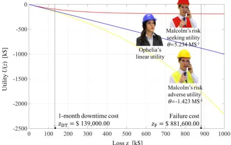
They also use the same interpretation model, i.e. they interpret identically the data from the monitoring system. After Malcolm estimates the state of the bridge, he may decide between two actions: Do nothing (DN), i.e. no special restrictions to traffic under and over the bridge; Close Bridge (CB), i.e. both Streicker Bridge and Washington Road are closed to traffic for the time needed for a thorough inspection, estimated to be 1 month. Finally, they agree that the costs z related to each action, for each scenario, are the ones estimated in (Glisic & Adriaenssens, 2010) and reported in Table 1.
Table 1: Costs per action and state.
Scenario U Scenario D Action DN z=0,0 k$ zF=881,6 k$ Action CB zDT=139,8 k$ zDT=139,8 k$
However, they differ in their utility functions, i.e. the weight they apply to the possible economic losses. Ophelia the owner is risk neutral, meaning that according to her a negative utility is linear with the incurred loss. Conversely, the behaviour of Malcolm can be risk adverse, i.e. his negative utility increases more than proportionally with the loss, or risk seeking, i.e. his negative utility increases less than proportionally with the loss. It is possible to describe mathematically these behaviours using the Arrow-Pratt’s utility model (Arrow, 1965) , where the different aptitude of an agent is encoded in the coefficient of Absolute Risk Aversion (ARA) θ. Fig. 2 shows the linear utility function of Ophelia and both Malcom’s behaviours: θ = -1.423 M$-1 if we model him as risk adverse, θ = 5.234 M$-1 if he is risk seeking.
Figure 2: Representation of the utility functions.
3.1. Risk adverse
In this first case we consider Ophelia’s utility function linear, i.e. risk neutral, while Malcolm’s one concave, according to his risk adverse behavior. Table 2 shows their consequent utilities.
Table 2: Ophelia’s and Malcolm’s loss perception.
Ophelia the owner RISK NEUTRAL Scenario U Scenario D DN (𝑂)𝑈(𝑧)=0,0 k$ (𝑂)𝑈(𝑧𝐹)=-881,6 k$
CB 𝑈(𝑧
𝐷𝑇) (𝑂)
=-139,8 k$ 𝑈(𝑧𝐷𝑇) (𝑂)
=-139,8 k$
Malcolm the manager RISK ADVERSE Scenario U Scenario D DN (𝑀)𝑈(𝑧)=0,0 k$ (𝑀)𝑈(𝑧𝐹)=-1762,9k$
CB 𝑈(𝑧
𝐷𝑇) (𝑀)
=-154,9 k$ 𝑈(𝑧𝐷𝑇) (𝑀)
[image:4.612.319.553.317.464.2]Before the monitoring system is installed, if we consider Ophelia alone, she would always choose to close the bridge when her utility related to the action CB is less negative than the utility of action DN, or rather:
𝑢CB (O)
≥ (O)𝑢DN, (8)
𝑈(𝑧𝐷𝑇)
(O) ≥ 𝑈(𝑧
F)
(O) ∙ P(D). (9)
According to Eq. (8) and Eq. (9), we can obtain Ophelia’s and Malcom’s prior probability thresholds, (O)r and (M)r respectively, which give us the probability value of damage after which is always more convenient for them to close the bridge a priori:
P(D) ≥ 𝑈(𝑧𝐷𝑇) (O)
𝑈(𝑧F)
(O) = 𝑟
(O) = 0.16. (10)
P(D) ≥ 𝑈(𝑧𝐷𝑇) (M)
𝑈(𝑧F)
(M) = 𝑟
(M)
= 0.09. (11)
Both prior thresholds are illustrated in Fig. 3; Malcolm’s one is clearly lower because of his risk adverse behavior. Moreover, we can observe that if we assume, as explain previously, P(D)=50% and P(U)=50% as prior probabilities, they both agree on closing the bridge as the best choice a priori.
Consider now the monitoring system installed. Ophelia’s and Malcolm’s pre-posterior expected utilities of doing nothing, respectively (O)u*
DN(ε) and (M)u*DN(ε), depend on the posterior probability of having the bridge damaged p(D|ε), which in turn depends on the monitoring observations ε, as reported in (Bolognani, et al., 2018). As rational agents, Ophelia and Malcolm will always take the decision related to the minimum loss. According to Eq. (4) and Eq. (7), we can calculate the VoI of Ophelia alone and her conditional VoI, i.e. if we consider Ophelia conditioned to Malcolm’s choices, respectively. The black lines in Fig. 4(a), (O)𝑢DNand (O)𝑢CB, are Ophelia’s prior utilities related to the action DN and CB respectively. The red curve, (O)𝑢∗ , is
her pre-posterior utility while the red dashed one,
𝑢∗
(O|M)
, her conditional pre-posterior utility, i.e. conditioned to Malcolm’s choices. Fig. 4(b) shows the unconditional and the conditional VoI (dashed curve) of Ophelia instead; all quantities are plotted in function of the probability of damage P(D). We can observe that both Ophelia’s unconditional and conditional VoI are maximum at her prior threshold (O)r, because the prior utilities takes over the posterior utilities and are responsible for the cusp in the graph of the VoI. However, even if the conditional VoI of Ophelia decreases compared to the unconditional one, we cannot find any value of P(D) for which it becomes negative. This happens because, due to Malcolm’s risk adverse behavior, he would always choose to close the bridge sooner than Ophelia. We can analyze better this situation plotting the posterior utilities of the two rational agents in function of the monitoring observations 𝛆 (Fig. 5). Due to their different behaviors, they perceive the risk differently and consequently they have two different strain thresholds. In particular, as shown in Fig. 5, we can demonstrate that even if they share exactly the same prior information, Malcolm, because of his risk adverse behavior, would always choose to close the bridge sooner than Ophelia ((M)ε̅
u = -111 με < (O)ε̅u =
126με). We remind that the unconditional VoI of Ophelia, according to Eq. (4), is equal to the area between the posterior utility(O)𝑢DN(y) and the horizontal line related to the action closing the bridge(O)𝑢CB(y); it corresponds to the blue area plus the dashed one, in Fig. 5. On the other hand, the conditional VoI, according to Eq. (7), is equal to the area between the conditional posterior utility (O|M)𝑢(y) and (O)𝑢CB(y); it corresponds to the blue area. We can observe that, if Malcolm is risk adverse and he chooses to CB sooner than Ophelia, the conditional VoI is smaller than the unconditional, but it can never become negative.
3.2. Risk seeking
again assume an Arrow-Pratt’s utility model, but this time with a positive ARA coefficient θ = 5.234 M$-1. By considering Ophelia still risk neutral, as from Table 2, the costs related to each action remain the same, while new Malcolm’s utilities are reported in Table 3.
Table 3: Malcolm’s loss perception.
Malcolm the manager RISK SEEKING Scenario U Scenario D DN (𝑀)𝑈(𝑧)=0,00 k$ 𝑈(𝑧
𝐹) (𝑀)
=-103,9 k$
CB 𝑈(𝑧
𝐷𝑇) (𝑀)
=-99,2 k$ (𝑀)𝑈(𝑧𝐷𝑇)=-99,2 k$
Ophelia’s prior threshold does not vary respect to Eq. (10), (O)r = 0.16, while Malcolm’s risk seeking priori threshold, according to Eq. (9), turns into (M)r = 0.53. This is clearly higher than his risk adverse prior threshold (M)r = 0.09, and also higher than Ophelia’s one because of his risk seeking behavior: his negative utility increases less than proportionally with the loss. The utility functions a priori with the thresholds are shown in Fig. 6.
Consider now the monitoring system installed and all the assumptions about the VoI made previously. Fig. 7(a) shows Ophelia prior and pre-posterior utilities, while Fig. 7(b) her conditional and unconditional VoI. Again, we can observe that both of these quantities are maximum at Ophelia prior threshold, (O)r = 0.16, and as they reach the top of the curve, they tend to decrease. Again, the prior utilities of Ophelia related to the action CB and DN are responsible for the cusps of the graph. However, in contrast to the previous case, now the conditional VoI of Ophelia (dashed line), not only decreases compared to the unconditional one (solid line), but we can also find a range of P(D) where it becomes negative.
In detail, by modelling Malcolm as risk seeking, we can always find a specific value of the damage probability (O|M)P(D)lim after which the
conditional VoI of Ophelia is negative or equal to zero. By analyzing it from a mathematical point of view, we can obtain (O|M)P(D)lim from:
𝑉𝑜𝐼
(O|M) = (O|M) ∗𝑢 −(O|M)𝑢 ≤ 0, (12)
which, solved in terms of P(D), provides us the following inequality:
P(D) ≤ F𝜀|U( 𝜀̅
(M)
) 𝑟−1
(O) ∙ F
𝜀|D((M)𝜀̅(PDM,𝑗)) − F𝜀|D((M)𝜀̅) + F𝜀|U((M)𝜀̅)
, (13)
where, Fε|D((M)𝜀̅) and Fε|U((M)𝜀̅) are the cumulate distributions for the damage and undamaged scenario respectively, while (O)r is Ophelia’s prior threshold. In Eq. (13), when P(D) starts to be greater than the member on the right side, the conditional VoI of Ophelia becomes negative. We identify this threshold as (O|M)P(D)lim, whichin this
specific case is equal to 0.48. This means that, if we model Malcolm the manager as risk seeking, and we assume a priori a damage probability higher than (O|M)P(D)lim=0.48, we are pretty sure to
find a negative values of the conditional VoI. Moreover, if we plot Ophelia’s and Malcolm’s posterior utilities, in function of the monitoring observations, we find again two different strain thresholds. In detail, as shown in Fig. 8, Malcolm, would choose to close the bridge later than Ophelia ((M) ε̅
u =464 με > (O) ε̅u =126 με ).
Ophelia’s threshold has remained obviously the same, while Malcolm’s one is increased because of his risk seeking behavior. So, there is a very wide range of values, from 126 to 464 με , whereby Malcolm would keep the bridge open in disagreement with Ophelia, who believes this is a dangerous practice which can potentially result is a big loss. Indeed, from Fig. 8 we can observe that after her threshold, Ophelia is forced to proceed along her posterior curve related to the action DN,
𝑢DN(y) (O)
, until Malcolm’s threshold, even if it would be more convenient for her to close the bridge. According to Fig. 8, the conditional VoI is equal to the blue area less the red one. Since we chose P(D)=50%, greater than (O|M)P(D)
lim, the red
Figure 3: Representation of Ophelia’s and Malcom’s utility functions a priori (i.e. without monitoring).
Figure 4: Representation of Ophelia’s and Malcom’s prior and preposterior utilities in function of P(D) (a); respective VoI (b).
[image:7.612.320.553.283.457.2]Figure 5: Representation of Ophelia’s and Malcom’s preposterior utilities u* in function of monitoring data.
Figure 6: Representation of Ophelia’s and Malcom’s utility functions a priori (i.e. without monitoring).
Figure 7: Representation of Ophelia’s and Malcom’s prior and preposterior utilities in function of P(D) (a); respective VoI (b).
[image:7.612.60.293.285.457.2] [image:7.612.60.292.503.669.2] [image:7.612.321.551.507.671.2]4. CONCLUSIONS
The benefit of SHM can be quantified using the concept of the Value of Information. In its calculation, a commonly understood assumption is that the individual who decide on the installation of the monitoring system, the owner, is the same rational agent who will later use it, the manager. With this assumption, the VoI is never negative, according to the assumption that “information can’t hurt”. On the other hand, it has been demonstrated that two different rational agents may be involved in the decision process. In this contribution, we demonstrate that under appropriate combination of prior information and utility functions, the conditionalVoI,i.e. the VoI of the owner conditioned to the manager choices, could be negative. In general, this can happen when the owner perceives the monitoring information as damaging, and then he/she believes that the monitoring system can seriously mislead the decision of the manager. Regarding the specific real-life case study about the Streicker Bridge, it turned out that it is possible to obtain a negative conditional VoI if we model Malcolm with a risk seeking behavior. Indeed, even if the two rational agents a priori share exactly the same information and agree on their choices, Malcolm would choose a posteriori to close the bridge later than Ophelia, because of his behavior. For this reason, she is forced to leave the bridge against her will, even if it would be more convenient for her to close it. Ophelia believes this is a dangerous practice that can potentially result is a big loss; consequently, we find a wide range of the damage prior probability in which the VoI results negative. On the other hand, if we model Malcolm with a risk adverse behavior, the VoI is never negative. In conclusion, we want to highlight that a negative VoI is exactly the amount of money the owner is willing to pay to prevent the manager using the monitoring system.
REFERENCES
Arrow, K. J., 1965. Aspects of the Theory of Risk Bearing. Helsinki: Yrjo Jahnssonin Saatio.
Bernal, D., Zonta, D. & Pozzi, M., 2009. An examination of the ARX as a residual generator for damage detection. s.l.
Bolognani, D. et al., 2018. Quantifying the benefit of strutural health monitoring: what if the manager is not the owner?. Structural Health Monitoring. Cover, T. M. & Thomas, J. A., 2012. Elements of information theory. s.l.:John Wiley & Sons.
DeGroot, M. H., 1984. Changes in utility as information. Theory and Decision,17(3),287-303. Glisic, B. & Adriaenssens, S., 2010. Streicker Bridge: initial evaluation of life-cycle cost benefits of various structural health monitoring approaches. s.l.
Glisic, B. & Inaudi, D., 2012. Development of method for in-service crack detection based on distributed fiber optic sensors. Structural Health Monitoring, 11(2), pp. 696-711.
Lindley, D. V., 1956. On a measure of the information provided by an experiment. 27(4), pp. 986-1005.
Pozzi, M., Malings, C. & Minca, A. C., 2017. Negative value of information in systems' maintenance. ICOSSAR 2017,Vienna, Austria. Pozzi, M., Zonta, D., Wang, W. & Chen, G., 2010. A framework for evaluating the impact of structural
health monitoring on bridge management.
Philadelphia.
Raiffa, H. & Schlaifer, R., 1961. Applied Statistical Decision Theory. s.l.:Clinton Press.
Straub, D. & Faber, M., 2005. Risk based inspection planning for structural systems. Structural safety, 27(4), pp. 335-55.
Thoft-Christensen, P. & Sorensen, J., 1987. Optimal strategy for inspection and repair of structural systems. Civil Eng. System, 4, 94-100.
Thons, S., 2017. On the Value of Monitoring Information for the Structural Integrity and Risk Management. Computer-Aided Civil and Infrastructure Engineering.