Power losses in electrical topologies for a multi-rotor wind turbine system

Power Losses in Electrical Topologies for a Multi-Rotor

Wind Turbine System

Ingvar Hinderaker Sunde1, Raymundo E. Torres-Olguin2, Olimpo Anaya-Lara3

1_{Department of Electric Power Engineering, Norwegian University of Science and}

Technology, Trondheim, Norway

2_{Department of Energy Systems, SINTEF Energy Research, Trondheim, Norway} 3_{University of Strathclyde, Glasgow, United Kingdom}

E-mail: ingvarhs@stud.ntnu.no

1. Introduction

Wind power is one of the most important energy resources worldwide. In 2017, 55 % of the new installed power capacity was wind power, and the offshore wind energy increased with 101 % [1]. Moreover, it is likely that the cumulative installed wind power will exceed 200 GW by the end of 2020 and, that of this, offshore wind will account for 25% [2].

Together with this increasing cumulative installed capacity, also the turbine sizes are increasing. In 2017, the average installed turbine rating was 2.7 MW for onshore applications, and 5.8 for offshore applications [1], the latter an increase of 39% from the year before [2]. Based on this, the development is expected to continue, which can turn out to be challenging for several reasons [3, 4]. The mechanical stress on the structure will increase with increasing blade size. Mechanical problems are anticipated and installation and maintenance may be more challenging. In addition, the high amount of material needed for the whole structure with these dimensions may be challenging to obtain. The raw materials and rare earth minerals used for production are getting more and more scarce due to the increasing demand [5]. It will also increase the costs, making it difficult to keep reducing the levelized cost of energy (LCOE).

As a suggested solution to this challenge, P. Jamieson proposed the Multi-Rotor Wind Turbine-system as a part of the FP7 INNWIND.EU project [6, 7], which consists of several rotors connected all together at the same platform. Such a system can be visualized in Fig. 1. The multi-rotor concept is stated to be beneficial in many ways, in terms of reduced weight in the nacelle and blade, easier installation, transport and maintenance due to smaller components, as well as higher reliability in case of faults, because a fault does not require the whole device to shut down [8]. However, the complexity of the whole system may be extensive and challenging. In this study, three possible electrical topologies are presented. These are implemented in Simulink, together with a loss calculation method which is also presented here. Further, the results from the simulations are presented and briefly discussed.

Fig. 1: Model of a multi-rotor wind turbine system, consisting of 45 rotors [6].

2. Proposed Topologies

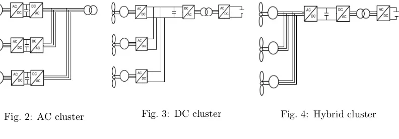
A theory review of electrical configurations was performed. The published literature regarding offshore wind farm collector systems [9, 10, 11] were used, as this can be considered as similar to a multi-rotor system. Some key differences are however present, such as much shorter inter-connected cables and the needlessness for subsea cables.

collecting the rotors in clusters, which is are also regarded as beneficial in this study. Three topologies were then selected and are further presented here.

Fig. 2: AC cluster Fig. 3: DC cluster Fig. 4: Hybrid cluster

2.1. AC cluster

The cluster consisting of a back-to-back converter for each turbine is here called the AC cluster. This can be seen in Fig. 2. The back-to-back converters allow individual control of each turbine, making it possible for each of them to operate in the optimal point of operation. Therefore, the machine side converter is controlling the active and reactive power of the turbine, while the grid-side converter is controlling the reactive power and the voltage of the DC link. The implementation and control are based on the model used in [4]. The three turbines present in this specific configuration are connected together in parallel, while in AC, and is meant to represent one cluster of a larger system. The collection is performed at a voltage level of 690 V, so a transformer is needed to further step up the voltage before connecting to other cluster and transmission.

2.2. DC cluster

The cluster consisting of just one AC-to-DC converter for each turbine is here called the DC cluster. This can be seen in Fig. 3. Also here, these converters allow individual control of each turbine, making it possible for each of them to operate in the optimal point of operation, thus it is controlling the active and reactive power. The control implementation of this converter is the same as used for the machine converter in the AC cluster. Further, the three turbines are connected together in parallel, while in DC. This keeps the voltage constant at 690 V. Also a series connection, or a combination could be used. This makes it possible to step up the voltage without the use of a transformer but increases the complexity and requires the use of by-passing techniques.

Fig. 5: Overall scheme for AC voltage control

2.3. Hybrid cluster

The cluster consisting of connecting in AC without any individual converters is here called the hybrid cluster. This can be seen in Fig. 4. This is proposed in order to investigate how the reduced number of converters trades off with the reduced control abilities. The first converter, controlling the active and reactive power as in the AC and DC cluster, now needs to control three turbines. Further, the same DC-to-DC converter as in the DC cluster is used, with its same control. The idea is that the wind conditions may not vary too much within the distances these rotors are apart. Then it could be possible to have all the three turbines operate equal, reducing the efficiency, but also the size and weight of the system.

If this can be beneficial may be questionable, but this topology is still included for investigation. As this study is limited to quite simplified systems and stationary conditions, the challenges in this topology will probably not be that visible but will be further analysed in future studies.

3. Power loss calculation

The power converters used in wind power application, consist mostly of IGBTs and diodes, so-called freewheeling diodes, in pairs. Therefore, the total losses are the sum of the losses in the IGBTs and in the diodes are according to

Ploss=PIGBT +Pdiode (1)

where PIGBT is the power losses in the IGBT andPdiode the power losses in the diode. The

semiconductor can either be conducting or blocking and has two possible transition states, the turn-on and turn-off. All of these cause power losses which can be found based on the derivations done in [13, 14].

3.1. Conduction losses

The voltage-current characteristics can be linearly approximated, obtaining the on state voltage of the device using the threshold voltage Vsw,o, and iC, the instantaneous current through the

on state resistanceRC for the IGBT, yielding

The same yields for the freewheeling diode, giving

vD(iD) =VD,o,+RD·iD (3)

These values can normally be found in the datasheet of a device. As can be seen from typical datasheets for IGBTs and diodes, the on-state diode and collector-emitter voltages, as well as the on-state resistors are dependent on the junction temperature. Normally, datasheets include data for different temperatures, so also these parameters can be found by the help of linear approximations

Vsw,0(Tj) =Vsw,00·(1 +αV sw0·(Tj−Tj0)) (4)

RC(Tj) =RC0·(1 +αRC·(Tj−Tj0)) (5)

whereαV sw0andαRC are the temperature coefficients of the threshold voltage and on-state

resistance,Vsw,00 andRC0 are the threshold voltage and on state resistance at a fixed reference junction temperature Tj0. Further, the instantaneous values of the power losses for an IGBT can be found to be

pcond,igbt(t) =vsw(t)·iC(t) =Vsw,o,(Tj)·iC(t) +RC(Tj)·i2C(t) (6)

which can further can be expressed to find the average losses as

Pcond,igbt=

1 Tsw

Z Tsw

0

pcond,igbt(t)dt=Vswo,0(Tj)·IC,avg+RC(Tj)·IC,rms2 (7)

whereIC,avg andIC,rms are the average and RMS currents in the IGBT and Tsw the time

of a switching period. In the diode, the same can be found, hence

pcond,D(t) =uD(t)·iD(t) =uD,o,(Tj)·iD(t) +RD(Tj)·i2D(t) (8)

Pcond,D =

1 Tsw

Z Tsw

0

pcond,D(t)dt=uD,o,(Tj)·ID,avg+RD(Tj)·ID,rms2 (9)

where the IGBT parameters are replaced with the diode parameters.

3.2. Switching losses

The switching losses are found on the dissipated energy due to the commutation for both turn-on and turn-off. For diodes, the turn-on energy mostly consists of the reverse recovery energy, while the turn-off energy is mostly neglected. However, the IGBTs have significant energy dissipation in both the turn-on and turn-off phases. In general, the switching energy in turn-on can be written as

Esw,on =Esw0,on·(1 +αEon·(Tj−Tj0)) (10)

where αEon is the temperature coefficient of commutation energy loss at turn on and the term

Esw0,on can be found as

Esw0,on=vswb·(KEon0+KEon1·iswa+KEon2·i2swa) (11)

whereEsw0,onis the commutation energy loss at turn on,vswb is the voltage in the device right

energy related to the switching can be turned to power by multiplying the number of switching per second, the switching frequency fsw. The same procedure is followed to find the turn-off

losses, and this results in the two equations

Psw,on =fsw·Esw,on=fswEsw0,on·(1 +αEon·(Tj−Tj0)) (12)

Psw,of f =fsw·Esw,of f =fswEsw0,of f ·(1 +αEof f ·(Tj−Tj0)) (13)

whereEsw,on and Esw,of f are found from equation 11 and the equivalent equation for the

turn off for the IGBT respectively. For the diode,Esw,of f is neglected, andEsw,onis claimed to

consist of mostly the reverse-recovery energy, which is found by

Esw,on,D=

1

4QrrUDrr (14)

whereQrrrepresents the recovered charge andUDrris the voltage across the diode during reverse

recovery.

3.3. Total power electronic losses

In total, equations can be set up to show the total losses in both the IGBTs and the diodes. To get the losses for the whole converter, the equations must be multiplied with the numberN of IGBTs and diodes in the actual converter. Then the total losses will be

PIGBT =N(Vsw0(Tj)·IC,av+RC(Tj)IC,rms2 + (Esw,on+Esw,of f)fsw) (15)

PD=N(VD,0(Tj)·ID,av+RD(Tj)ID,rms2 +Esw,onfsw) (16)

3.4. Implemented loss calculation method

In order to quantify the power losses inside of the converters, the models from [15] were used and modified to fit a two-level converter. This model obtains the signal measurements of both IGBT and diode pair in one half-bridge. These signals are used to specify the voltage and the current in the IGBTs and in the diodes. Further, these signals are divided into loss calculations blocks for the IGBT and diode respectively. A simplification done is using just one IGBT and diode module for each part of the half bridge. Normally in these types of devices, there are several modules connected in series, in order to increase the possible voltage level. The tests are therefore kept within limits where they can operate with just one module.

The IGBT losses are separated into switching and conduction losses. The different losses are found, based on the parameters presented in their respective equations. These values are used to find the dissipated turn-on energy by interpolation with the help of look-up tables. The look-up tables is linked with datasheet of a specified IGBT module, defined in Matlab. From this, the dissipated energy from the switching is found and is transformed into power. For the conduction losses, the loop-up table finds the saturation voltage, which is multiplied with the current to obtain the power losses. The power is further injected into the thermal model which obtains the IGBT temperature.

4. Simulation results

Simulations for the different topologies were carried out. Due to the different voltage and current level in the different topologies as well as also within one topology, different IGBT and diode modules needed to be defined in Matlab. From the loss calculation blocks [15], three IGBT and diode-modules had been implemented in Matlab, based on their available datasheets. These were a 600V/150A module [16] from Fuji Electric, a 1700V/800A module [17] from ABB and a 3300V/250A module [18], also from ABB. A combination of these was sufficient to deal with the currents of the different systems but problematic for the voltage level after the step-up transformers. Therefore, another IGBT and diode module was implemented in Matlab, with the help of the datasheet of the module. This was a 6500V/600A module [19] from ABB, their single module with the highest voltage capability.

An important simplification in order to calculate these losses is that just one single IGBT and diode module is used for each switch. Hence in the three-phase bridge with 6 pulses, there are only six of these modules. In reality, multiple modules may be connected in series to increase the voltage level instead of using modules with a very high rating. This may influence the result, but was a necessity for limiting the complexity of the scope of this study.

The losses in the three topologies are presented below.

4.1. AC cluster

Since the turbines are operating equally and ideally, without any dynamic differences, the power losses in the different corresponding converters are equal. Therefore only one of each, the machine side and grid side converter are presented here. The machine side converter losses are presented in Fig. 6 and the grid side converter in Fig. 7.

Fig. 6: Machine side losses Fig. 7: Grid side converter

The power losses for one machine side converter are found to be stabilising at 1.6 kW, giving the percentage losses of

Ploss[%]= Ploss

Pin

·100%≈ 1.6kW

300kW·100% = 0.53% (17)

The total losses for one grid side converter are stabilising at 1.9 kW. This gives the percentage losses of

Ploss[%]= Ploss

Pin

·100%≈ 1.9kW

4.2. DC cluster

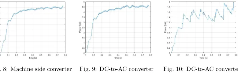
In the three machine side converters, the losses are equal due to their equality. Therefore, only one of the converter losses is presented here, in Fig. 8. The losses in the DC-to-AC and AC-to-DC converters are presented in Fig. 9 and Fig. 10 respectively.

Fig. 8: Machine side converter Fig. 9: DC-to-AC converter Fig. 10: DC-to-AC converter

The total power losses in one machine side converter are found to be stable at 1.6 kW, giving a percentage of losses of

Ploss[%]= Ploss

Pin

·100%≈ 1.6kW

300kW·100% = 0.53% (19)

The losses for the DC to AC side are found to be stable at around 4.5 kW, giving the percentage losses of

Ploss[%]= Ploss

Pin

·100%≈ 4.5kW

900kW·100% = 0.50% (20)

The module information in the 6500V/600A module used in the AC to DC side was implemented without the same precision level as the other three. Therefore, the curve showing the power losses are not as smooth. However, the losses are found to be stable at around 1.8 kW, giving the losses in percentage as

Ploss[%]= Ploss

Pin

·100%≈ 1.8kW

900kW·100% = 0.20% (21)

The last converter is experiencing very low current due to the step-up transformer. This, as it can be seen, has a big impact on the losses.

4.3. Hybrid cluster

Only one machine side converter is present, consisting of the power from three turbines. Thus the losses for this converter is presented in Fig. 11. The losses in the DC-to-AC and AC-to-DC converters are presented in Fig. 12 and Fig. 13 respectively. The total summarised losses stabilise at about 4.0 kW. This gives the percentage losses of

Ploss[%]= Ploss

Pin

·100%≈ 4.0kW

900kW·100% = 0.44% (22)

From the first part, the losses are found to be stable at a value of about 4.5 kW, giving the percentage losses of

Ploss[%]= Ploss

Pin

·100%≈ 4.5kW

Fig. 11: Machine side converter Fig. 12: DC-to-AC converter Fig. 13: AC-to-DC converter

The module information in the 6500V/600A module used in the AC to DC side is implemented without the same precision level as the other three. Therefore, also in the curve shown here, the power losses are not as smooth. However, the losses are found to be stable at around 1.9 kW, giving the losses in percentage as

Ploss[%]= Ploss

Pin

·100%≈ 1.9kW

900kW·100% = 0.21% (24)

Also here, as in the DC cluster, the converter losses are low due to the much lower current after the transformer.

5. Conclusion

From the results, it is observed that the power losses are at a low, and expected level. Summarised, they are also quite similar to each other. The machine and converter losses are similar in each topology, due to their similar output. The high voltage side in the DC-to-DC converter experiences low losses and can be because of low current.

This study excludes the transformer losses. These are expected to increase with frequency [20], so the use of a medium-frequency transformer in the DC-to-DC converter will probably give higher total power losses in the DC cluster and hybrid cluster topologies than the total power losses in the AC cluster, which is using a grid-frequency transformer. However, the trade-off between how much space and weight this may save and how much the losses are increased is of interested and need further investigation. This will be performed in further studies, together with increasing the complexity of the system in terms of the number of rotors, but also by investigating dynamic conditions and varying wind profiles. Then it can be more visible the challenges regarding the control of the different topologies. However, a way of obtaining the power losses within the power converters are obtained and proved to provide meaningful results. This can therefore also be used in future work on this topic, in order to find a suitable topology for the electrical configurations of a multi-rotor wind turbine system.

References

[1] WindEurope,Wind in power 2017 Annual combined onshore and offshore wind energy statistics, 2018 [2] WindEurope,Wind energy in Europe: Outlook to 2020, 2017

[3] Givaki K Different Options for Multi-Rotor Wind Turbine Grid Connection, The 9th International Conference on Power Electronics, Machines and Drives, 2018

[4] Pirrie P, Anaya-Lara O and Campos-Gaona D Electrical collector topologies for multi-rotor wind turbine systems, 2018

[6] Jamieson P, et alInnovative Turbine Concepts Multi-Rotor SystemINNWIND.EU, 2015

[7] Jamieson P and Branney MMulti-Rotors; A Solution to 20 MW and Beyond?Energy Procedia, Volume 24, 2012, Pages 52-59

[8] Verma P Multi Rotor Wind Turbine Design And Cost Scaling, 2014

[9] Lakshmanan P, Liang J and Jenkins N SAssessment of collection systems for HVDC connected offshore wind farms, Electric Power Systems Research Volume 129, 2015, Pages 75-82

[10] Quinonez-Varela G, Ault G W, Anaya-Lara O and McDonald J RElectrical collector system options for large offshore wind farmsIET Renewable Power Generation Volume 1, Issue: 2, 2007, Pages 107 - 114 [11] Srikakulapu R and U VElectrical Collector Topologies for Offshore Wind Power Plants: A Survey 2015

IEEE 10th International Conference on Industrial and Information Systems (ICIIS), 2015, page 338-343. [12] Gksu , Sakamuri J N, Rapp A C, Srensen P E, Sharifabadi KCluster Control of Offshore Wind Power

Plants Connected to a Common HVDC Station, Energy Procedia Volume 94, 2016, Pages 232-240 [13] Barrera-Cardenas R AMeta-parametrised meta-modelling approach for optimal design of power electronics

conversion systems: Application to offshore wind energyDoctoral thesis, 2015

[14] Graovac D and Prschel MIGBT Power Losses Calculation Using the Data-Sheet Parameters, 2009 [15] Mathworks Loss Calculation in a 3-Phase 3-Level Inverter Using

SimPower-Systems and Simscape https://www.mathworks.com/help/physmod/sps/examples/ loss-calculation-in-a-three-phase-3-level-inverter.html

[16] Fuji ElectricDatasheet:IGBT Module U-Series 600V/150A 2 in one-package 2MBI150U2A-060 [17] ABBDatasheet: ABB HiPak IGBT Module 1700V/800A 5SNE 0800M170100

[18] ABBDatasheet: ABB HiPak IGBT Module 3300V/250A 5SNG 0250P330305 [19] ABBDatasheet: ABB HiPak IGBT Module 6500V/600A 5SNG 0250P330305