City, University of London Institutional Repository
Citation
:
Myklebust, E., Jimenez-Ruiz, E. ORCID: 0000-0002-9083-4599, Chen, J., Wolf,
R. and Tollefsen, K. E. (2019). Knowledge Graph Embedding for Ecotoxicological Effect
Prediction. In: The Semantic Web – ISWC 2019: 18th International Semantic Web
Conference, Auckland, New Zealand, October 26–30, 2019, Proceedings. Lecture Notes in
Computer Science, 11779 (11778). (pp. 490-506). Cham: Springer. ISBN 978-3-030-30792-9
This is the accepted version of the paper.
This version of the publication may differ from the final published
version.
Permanent repository link:
http://openaccess.city.ac.uk/id/eprint/22930/
Link to published version
:
http://dx.doi.org/10.1007/978-3-030-30793-6
Copyright and reuse:
City Research Online aims to make research
outputs of City, University of London available to a wider audience.
Copyright and Moral Rights remain with the author(s) and/or copyright
holders. URLs from City Research Online may be freely distributed and
linked to.
City Research Online: http://openaccess.city.ac.uk/ [email protected]
Ecotoxicological Effect Prediction
Erik B. Myklebust1,2?, Ernesto Jimenez-Ruiz2,3, Jiaoyan Chen4, Raoul Wolf1, and Knut Erik Tollefsen1
1 Norwegian Institute for Water Research, Oslo, Norway 2
Department of Informatics, University of Oslo, Norway
3 Alan Turing Institute, London, United Kingdom 4
Department of Computer Science, University of Oxford, United Kingdom
Abstract. Exploring the effects a chemical compound has on a species takes a considerable experimental effort. Appropriate methods for es-timating and suggesting new effects can dramatically reduce the work needed to be done by a laboratory. In this paper we explore the suitabil-ity of using a knowledge graph embedding approach for ecotoxicological effect prediction. A knowledge graph has been constructed from publicly available data sets, including a species taxonomy and chemical classifi-cation and similarity. The publicly available effect data is integrated to the knowledge graph using ontology alignment techniques. Our experi-mental results show that the knowledge graph based approach improves the selected baselines.
Keywords: Knowledge graph·Semantic embedding·Ecotoxicology
1
Introduction
Extending the scope of risk assessment models is a long-term goal in ecotox-icological research. However, biological effect data is only available for a few combinations of chemical-species pairs.1Thus, one of the main efforts in ecotox-icological research is the design of tools and methods to extrapolate from known to unknown combinations in order to facilitate risk assessment predictions on a population basis.
The Norwegian Institute for Water Research (NIVA) is a leading Norwegian institute for fundamental and applied research on marine and freshwaters.2The Ecotoxicology and Risk Assessment programme at NIVA has through the last years developed a risk assessment system called RAdb.3 This system has been applied to several case studies based on agricultural/industrial runoff into lakes or fjords. However, the underlying relational database structure of RAdb has
?
Corresponding author: Erik B. Myklebust,[email protected]
1 Chemical and compound are used interchangeably. 2
NIVA Institute: https://www.niva.no/en
3
its limitations when dealing with the integration of diverse data and knowledge sources. This limitation is exacerbated when these resources do not share a common vocabulary, as it is the case in our ecotoxicology risk assessment setting. In this paper we present a preliminary study of the benefits of using Semantic Web tools to integrate different data sources and knowledge graph embedding approaches to improve the ecotoxicological effect prediction. Hence, our contri-bution to the NIVA institute is twofold:
(i) We have created a knowledge graph by gathering and integrating the relevant biological effect data and knowledge. Note that the format of the source data varies from tabular data, to SPARQL endpoints and on-tologies. In order to discover equivalent entities we exploit internal re-sources, external resources (e.g., Wikidata [21]) and ontology alignment (e.g., LogMap [12]).
(ii) We have evaluated three knowledge graph embedding models (TransE [5], DistMult [23] and HolE [17]) together with the (baseline) prediction model currently used at NIVA. Our evaluation shows a considerable improvement with respect to the baseline and the benefits of using the knowledge graph models in terms of recall andFβ=2 score. Note that, in the NIVA use case, false positives are preferred overfalse negatives (i.e., missing the hazard of a chemical over a species).
The rest of the paper is organised as follows. Section 2 provides some prelim-inaries to facilitate the understanding of the subsequent sections. In Section 3 we describe the use case where the knowledge graph and prediction models are applied. The creation of the knowledge graph is described in Section 4. Section 5 introduces the effect prediction models, while Section 6 presents the evaluation of these models. Finally, Section 7 elaborates on the contributions and discusses future directions of research.
2
Preliminaries
Knowledge graphs. We follow the RDF-based notion of knowledge graphs [4] which are composed by RDF triples hs, p, oi, where s represents a subject (a class or an instance), p represents a predicate (a property) and o represents an object (a class, an instance or a data value e.g., text, date and number). RDF entities (i.e., classes, properties and instances) are represented by an URI (Uniform Resource Identifier). A knowledge graph can be split into a TBox (ter-minology), often composed by RDF Schema constructors like class subsump-tion (e.g., ncbi:taxon/6668 rdfs:subClassOf ncbi:taxon/6657) and prop-erty domain and range (ecotox:affects rdfs:domain ecotox:Chemical),4 and an ABox (assertions), which contain relationships among instances (e.g., ecotox:chemical/330541 ecotox:affects ecotox:effect/202) and seman-tic type definitions (e.g.,ecotox:taxon/28868 rdf:type ecotox:Taxon).
RDF-4
based knowledge graphs can be accessed with SPARQL queries, the standard language to query RDF graphs.
Ontology alignment. Ontology alignment is the process of finding mappings or correspondences between a source and a target ontology or knowledge graph [10]. These mappings are typically represented as equivalences among the entities of the input resources (e.g.,ncbi:taxon/13402 owl:sameAs ecotox:taxon/Carya).
Embedding models. Knowledge graph embedding [22] plays a key role in link prediction problems where the goal is to learn a scoring functionS:E × R × E → R. S(s, p, o) is proportional to the probability that a triple hs, p, oi is encoded
as true. Several models have been proposed,e.g., Translating embeddings model (TransE) [5]. These models are applied to knowledge graphs to resolve miss-ing facts in largely connected knowledge graphs, such as DBpedia [14]. Embed-ding models have also been successfully applied in biomedical link prediction tasks (e.g., [3, 2]).
Evaluation metrics. We use (A)ccuracy, (P)recision, (R)ecall, (Fβ) score to evaluate the models. They are defined as
A= tp+tn
tp+tn+f p+f n (1) P = tp
tp+f p (2)
R= tp
tp+f n (3)
Fβ = (1 +β2)
P R
β2P+R (4) where tp, tn, f p, and f n stand for true positive, true negative, false positive, andfalse negative, respectively. Essentially, accuracy is the proportion of correct classifications. Recall is a measure of how many expected positive predictions were found by our model, and precision is the proportion of predictions that were correctly classified.Fβis a combined measure of precision and recall.β = 1 gives equal weight, whileβ <1 favours precision andβ >1 favours recall. Here we useFβ=1 (F1 in short) andFβ=2.
As the above metrics all depend on a selected threshold, we also use area under the receiver operating characteristic (ROC) curve (AUC) to measure and compare the overall pattern recognition capability of the prediction models. ROC is the curve of true positive rate (tp/(tp+f n), i.e., recall) and false positive rate (f p/(f p+tn)), with the threshold ranging from 0 to 1 using a small step. AUC is the area under this curve, its values range between 0 and 1. Larger AUC indicates higher performance.
3
NIVA use case: ecotoxicology and risk assessment
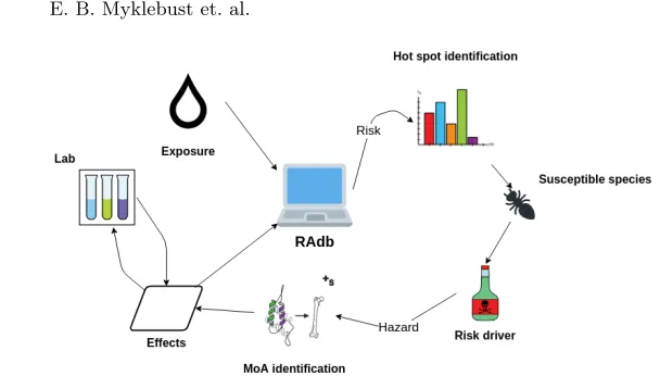
ecosys-Fig. 1: NIVA risk assessment pipeline.
Proportion Abbreviation Description
0.21 NR Not reported
0.17 NOEL No-observable-effect-level
0.16 LC50 Lethal concentration for 50% of test population 0.14 LOEL Lowest-observable-effect-level
0.05 NOEC No-observable-effect-concentration
0.05 EC50 Effective concentration for 50% of test population 0.04 LOEC Lowest observable effect concentration
0.03 BCF Bioconcentration factor
0.02 NR-LETH Lethal to 100% of test population 0.02 LD50 Lethal dose for 50% of test population
0.11 Other
Table 1: The 10 most frequent outcomes in ECOTOX effect data.
tems. Risk assessment is the result of the intrinsic hazards of a substance com-bined with an estimate of the environmental exposure (i.e., Hazard + Expo-sure = Risk).
The Computational Toxicology Program within NIVA’s Ecotoxicology and Risk Assessment section aims at designing and developing prediction models to assess the effect of chemical mixtures over a population where traditional laboratory data cannot be easily acquired.
Figure 1 shows the risk assessment pipeline followed at NIVA. Exposure is data gathered from the environment, whileeffects are hypothesis that are tested in a laboratory. These two data sources are used to calculate risk, which is used to find (further) susceptible species and the mode of action (MoA) or type of impact a compound would have over those species. Results from the MoA analysis are used as new effect hypothesis.
[image:5.612.145.449.93.266.2]Most commonly, the mortality rate of the population is measured at each time interval until it becomes a constant. Although the mortality at each time in-terval is referred to asendpoint in the ecotoxicology literature, we useoutcome
of the experiment to avoid confusion. Table 1 shows the typical outcomes and their proportion within the effects data. To give a good indication of the toxicity to a species, these experiments need to be repeated with increasing concentra-tions until the mortality reaches 100%. However, this is time consuming and is generally not done (sola dosis facit venenum). Hence, some compounds may ap-pear more toxic than others due to limited experiments. Thus, when evaluating prediction models, (higher values of) recall are preferred over precision.
Risk assessment methods require large amounts of effect data to efficiently predict long term risk for the ecosystems. The data must cover a minimum of the chemicals found when analysing water samples from the ecosystem, along with covering species present in the ecosystem. This leads to a immense search space that is close to impossible to encompass in its entirety. Thus, it is essen-tial to extrapolate from known to unknown combinations of chemical-species and suggest to the lab (ranked) effect hypothesis. The state-of-the-art within ef-fect prediction are quantitative structureactivity relationship models (QSARs). These models have shown promising results for use in risk assessment,e.g., [19]. However, QSARs have limitations with regard the coverage of compounds and species. These models use some chemical properties, but they usually only con-sider one or few species at a time. In this work we contribute with an alternative approach based on knowledge graph embeddings where the knowledge graph provides a global and integrated view of the domain.
Currently, the NIVA RAdb is under redevelopment, giving opportunities to include sophisticated effect prediction approaches, like the one presented in this paper, as a novel module for improving domain wide regulatory risk assessment.
4
A knowledge graph for toxicological effect data
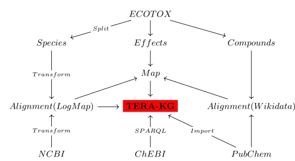
Risk assessment involves different data sources and laboratory experiments as shown in Figure 1. In this section we describe the relevant datasets and their integration to create the Toxicological Effects and Risk Assessment (TERA) knowledge graph (see Figure 2).
4.1 The ECOTOX database
We rely on the ECOTOXicology database (ECOTOX) [9]. ECOTOX consists of
ECOT OX
Species Ef f ects Compounds
M ap
Alignment(LogM ap) TERA-KG Alignment(W ikidata)
N CBI ChEBI P ubChem
Split
T ransf orm
[image:7.612.150.452.108.273.2]T ransf orm SP ARQL Import
Fig. 2: Data sources in the TERA knowledge graph. Compound classification is available from PubChem. Chemical class hierarchy comes from the ChEMBL SPARQL endpoint. Compound literals are gathered from PubChem REST API and transformed into triples. ECOTOX and PubChem identifiers are aligned using the Wikidata SPARQL endpoint. ECOTOX and NCBI taxonomies are aligned using LogMap.
test id reference number test cas species number
1068553 5390 877430 (2,6-Dimethylquinoline) 5156 (Danio rerio)
2037887 848 79061 (2-Propenamide) 14 (Rasbora heteromorpha)
result id test id endpoint conc1 mean conc1 unit
98004 1068553 LC50 400 mg/kgdiet
2063723 2037887 LC10 220 mg/L
Table 2: ECOTOX database entry examples.
Table 2 contains an excerpt of the ECOTOX database. ECOTOX includes information about the compounds and species used in the tests. This infor-mation, however, is limited and additional (external) resources are required to complement ECOTOX.
The number of outcomes per compound and species varies substantially. For example, there are 1,881 experiments where the compound used issulfuric acid, and 9,436 experiments wherePimephales promelas (fathead minnow) is the test species. The median number of experiments per chemical and species are 3 and 6, respectively. Figure 3 visualises a subset of the outcomes, here the zero values are either no effect or missing. This figure shows certain features of the data,
e.g., that compounds are more diversely used than species and that compound similarity is closely correlated to effects with regards to a species.
Fig. 3: ECOTOX effects data.xandy-axis represent individual species and chem-icals sorted by similarity. Similarities are given by Equations (6) and (7) in Sec-tion 5.1.i.e., chemicalsci ∈Care indexed such thatS0,1> S1,2>· · ·> Sn−1,n. Showing only chemicals and species that are involved in 25 or more experi-ments. Values relate to mortality rate of the test population, i.e., LC50 corre-sponds to 0.5.
have multiple experiments per species, the mean and standard deviation of risk to a species can be calculated. However, if there is only one experiment for a compound-species pair we cannot calculate a standard deviation, such that the risk assessment is featureless. Therefore, estimating new effects is important to represent the natural variability of the effect data.
4.2 Dataset integration into the TERA knowledge graph
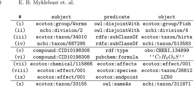
Figure 2 shows the different datasets and their transformation that contribute in the creation of the TERA knowledge graph. For example Triples(vii)-(ix)in Table 3 have been created from the ECOTOX effect data.
# subject predicate object (i) ecotox:group/Worms owl:disjointWith ecotox:group/Fish (ii) ncbi:division/2 owl:disjointWith ncbi:division/4 (iii) ecotox:taxon/34010 rdfs:subClassOf ecotox:taxon/hirta
(iv) ncbi:taxon/687295 rdfs:subClassOf ncbi:taxon/513583 (v) compound:CID10198308 rdf:type obo:CHEBI 134899 (vi) compound:CID10198308 pubchem:formula ‘‘C7H6O6S’’
(vii) ecotox:chemical/115866 ecotox:affects ecotox:effect/001 (viii) ecotox:effect/001 ecotox:species ecotox:taxon/26812
[image:9.612.137.459.93.239.2](ix) ecotox:effect/001 ecotox:endpoint LC50 (x) ecotox:taxon/33155 owl:sameAs ncbi:taxon/311871
Table 3: Example triples from the TERA knowledge graph
extract the classification (provided by the ChEBI ontology [6]) for the relevant PubChem compounds. For example Triples (v) and(vi) in Table 3 come from the integration with PubChem and ChEMBL.
Aligning ECOTOX and NCBI. The species lineage in ECOTOX is not com-plete and therefore this (missing) information has been complemented with the NCBI taxonomy [16], a curated classification of all of the organisms in the public sequence databases (around 10% of the species on Earth). The tabular data pro-vided for the ECOTOX species and the NCBI taxonomies has been transformed into subsumptions and disjointness triples (see first four triples in Table 3). Leaf nodes are treated as instance entities.
Since there does not exist a complete and public alignment between ECO-TOX species and the NCBI Taxonomy, we have used the LogMap [11, 12] ontol-ogy alignment systems to index and align the ECOTOX and NCBI vocabularies. ECOTOX currently only provides a subset of the mappings via its web search interface. We have gathered a total of 929 ground truth mappings for validation purposes. The lexical indexation provided by LogMap left us with 5,472 pos-sible NCBI entities to map to ECOTOX (we focus only on instances,i.e., leaf nodes). LogMap identified 4,681 (instance) mappings to ECOTOX (∼40% of its entities) covering all 929 mappings from the (incomplete) ground truth, thus, an estimated recall of 100%. The mappings computed by LogMap have been included to the TERA knowledge graph as additional equivalence triples (see Triple(x)in Table 3 as example).
5
Effect prediction models
c1 s1
CA SA
CR c2 s2 SR
CB SB
c3 s3
type
Af f ects
N ot af f ects
type
subClassOf subClassOf
type
type type
subClassOf
type
Af f ects Af f ects
[image:10.612.177.438.118.250.2]type
Fig. 4: The effect prediction problem. Lowercasesjandciare instances of species and compounds, while uppercase denote classes in the hierarchy. Solid lines are observations and dashed lines are to be predicted.i.e., doesc2 affects1?
asAffects andNot affects in the figure, to predict whether or not new proposed chemical-species pairs aretrue (Affects) orfalse (Not affects).5
Effect data sampling. A balance between positive and negative effect data samples is desired, therefore, we choose outcomes in categories (refer to Table 1): NOEL, LCp, LDp, NR-LETH, and NR-ZERO (p ranges from 0 to 100). We are only concerned about the mortality rate in experiments, consequently, we treat LC* and LD* identically. In addition, NR-LETH is treated as LC100. For simplicity, we treat the effects as binary entities. Hence, the outcome for a compound-species pairc, sis defined as
f(c, s) =
(
1 if (c, s)∈LCp∪LDp∪NR-LETH
0 if (c, s)∈NOEL∪NR-ZERO. (5)
For example, according to Figure 4, f(c1, s1) = 1 (i.e., c1 affects s1) and
f(c1, s2) = 0 (i.e.,c1 does not affectss1), whilef(c2, s1) is unknown and thus a prediction is required for this chemical-species pair.
Knowledge graphs. We rely on the TERA knowledge graph (see excerpts in Table 3 and Figure 4) to feed the knowledge graph embedding algorithms. For simplicity we discard the ECOTOX species entities that have not a correspon-dence to NCBI. Note that we currently do not consider literals.
5.1 Baseline model (M1)
This (baseline) prediction model is based on the current prediction method used at NIVA. The basic idea of this method is to find the nearest-neighbour from the
5
observed samples. In this context, the nearest neighbours are defined by hierar-chy distance for species and similarity for compounds. Therefore, we first define a adjacency matrix for the taxonomy and a similarity matrix for compounds.
Ai,j=
1
|P(si, r)|+|P(sj, r)| −2|P(si, r)∩P(sj, r)|+ 1
(6)
whereris the taxonomy root,P(x, r) is the classes in the path fromxtor, and|·|
denotes the cardinality. One basic approach to calculate the chemical similarity is using the Jaccard index of the binary fingerprints of the compounds [18]. Hence, the similarity matrix is defined as
Si,j=J(ci, cj) =
|(Fi)2∩(Fj)2|
|(Fi)2∪(Fj)2|
(7)
We define a matrixE∈R|C|×|T|, whereCandT denote the set of compounds
and species respectively.E contains all the observed effects (training set):
Ei,j=
(
1 if (ci, affects,sj)
0 else (8)
We can then make the prediction withA,S, andE, as shown in Algorithm 1. The algorithm terminates whentmax neighbours are visited orp >0.
5.2 Multilayer perceptron (M2)
Our second prediction model is a Multilayer perceptron (MLP) network withn
hidden layers. The model can be expressed as:
y0= [ec,es] (9) yt=ReLu(yt−1Wt+bt) (10)
ˆ
y=σ(ynWn+bn) (11) where t = 1,2, ..., n. [·,·] denotes vector concatenation. ReLu is the rectifier function andσis the logistic sigmoid function.Wtare the weight matrices and
btare the biasses for each layer.ec,es∈Rk are the embedded vectors ofc and
s. For example ec is defined as
ec =δcWC (12) whereδcis the one-hot encoded vector for entityc,WC∈R|C|×kis an embedding
transformation matrix to learn.
A dropout layer is stacked after each hidden layer to prevent the network from overfitting. The model is optimised using ADAGRAD [8] with the following log loss function:
L(y,yˆ) =−1
N
N
X
i=1
Input:E,A,S,ci,sj
Output:p, effect prediction forci, sj
i0, j0←i, j;
t1←tmax;
p←Ei,j ; // 0 if no overlap between train and test
whilet1>0do
i0←arg maxk6=iSi,k; // find index of most similar compound
A0←A;t2←tmax; // copy A and reset counter
resetj; // reset to j in input sj
whilet2>0do
j0←arg maxk6=jA 0
j,k; // index of closest specie
p←max (p, Ei0,j0); // update prediction
A0j,j0←0; // set seen indices to zero
t2←t2−1;
if p >0then returnp;
i, j←i0, j0; // update
end
Si,i0 0 ←0; // set seen indices to zero
t1←t1−1;
end returnp;
Algorithm 1: Baseline prediction model algorithm (M1).
5.3 Knowledge graph (KG) embedding and MLP (M2?)
We have extended the MLP model (M2) by feeding it with the TERA KG-based embeddings of c (i.e., the chemical) and s(i.e., the species), which encode the information of the taxonomy and compound hierarchies, among other semantic relationships. Note that the TERA knowledge graph also includes similarity triples about compounds. These triples represent pairs of compoundsci andcj where their similaritySi,j (as in Equation 7) is above a thresholdφ.
The embeddings are learned by applying the scoring function from one of DistMult [23], HolE [17], and TransE [5]. TransE was selected as it provides a very intuitive model. DistMult was included as it has shown state-of-the-art performance (e.g., [13]), while HolE was considered as it also encodes directional relations. The score function for DistMult is defined as
SD(s, p, o) =σ(eTsWpeo), Wp=diag(ep) (14) HolE uses a circular correlation score function, defined by
SH(s, p, o) =σ(erT[es?eo]), es?eo=F−1[F(es) F(eo)] (15) where F and F−1 are the Fourier transform and its inverse, xis the element-wise complex conjugate,denotes the Hadamard product. The final method is TransE, which has the score function
where||x|| is the norm ofx.es,ep andeoare the vector representation for the subject, predicate and object of a triple, respectively.
DistMult and HolE optimises for a score of 1 for positive samples and 0 for negative samples. Moreover, TransE scores positive samples as 0 and with no upper bound for negative samples. We modify the TransE score function to
ST0 = tanh (1/ST), such that limST→0S 0
T = 1 and limST→∞S 0
T = 0, to avoid modifying the labels.
The embeddings are used in the same network as theM2 model. We train the embeddings and the classifier simultaneously using log loss and ADAGRAD. Training simultaneously will optimise the embeddings with regards to both the knowledge graph triples and the classifier loss.
6
Effect prediction evaluation
Sampling.We split the effect data 50%/50% for train/test. To prevent test set leakage, those training inputs that appear in the test set are removed, resulting in a 70%/30% split.M?
2 can be trained with the entirety of the knowledge graph, which is ignored under effect prediction. The negative knowledge graph samples are generated by randomly re-sampling subject and object of a true sample, while maintaining the distribution of predicates. We generate four negative samples per positive sample.
M1model settings.We tested the performance ofM1with 6 choices of nearest neighbour (5, 10, 20, 30, 40, 50). In addition to Algorithm 1, we tested an alternative technique for iterating over the data. However, Algorithm 1 yielded better results. The most balanced results were found when using 30 neighbours. When using more than 30 neighbours recall increases, but accuracy and precision suffer from a considerable decrease since the use of more neighbours increases the false positive rate.
M2/M?2 model settings. The embedding dimension used inM2 and M2? was based on a search among sizes 16, 64, 128 and 256. We found no difference between these parameters forM2, therefore, 16 is chosen to aid faster training.
M?
2 used a larger amount of entities and needs a larger embedding space to capture the features of the data. The performance plateaued at 128, hence, this was chosen. The models (M2,M2?) were trained until the loss stops improving for 5 iterations. For M2? we used different loss weights for the embeddings and the effect predictor. These weights were chosen such that the embeddings and effects are learned at similar rates. DistMult and HolE used 0.5 and 1.0 as loss weights for embeddings and effects models, respectively, while TransE used equal weights. We used a dropout rate of 0.2 and a similarity threshold of 0.5. Note that in M?
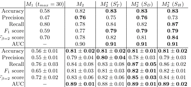
M1(tmax= 30) M2 M2?(ST0) M ?
2 (SD) M2?(SH)
Accuracy 0.58 0.82 0.83 0.83 0.83
Precision 0.47 0.76 0.75 0.76 0.73
Recall 0.80 0.78 0.84 0.82 0.87
F1 score 0.59 0.77 0.79 0.79 0.79
Fβ=2score 0.70 0.78 0.82 0.81 0.84
AUC − 0.90 0.91 0.91 0.91
Accuracy 0.56±0.01 0.81±0.02 0.81±0.02 0.81±0.01 0.81±0.02 Precision 0.55±0.01 0.79±0.04 0.80±0.04 0.78±0.03 0.79±0.03
Recall 0.76±0.03 0.84±0.08 0.83±0.08 0.87±0.05 0.86±0.02 F1 score 0.65±0.01 0.81±0.03 0.81±0.03 0.82±0.01 0.82±0.01
Fβ=2score 0.72±0.02 0.83±0.06 0.82±0.06 0.85±0.03 0.84±0.01
[image:14.612.153.469.114.258.2]AUC − 0.89±0.01 0.88±0.01 0.89±0.01 0.89±0.02
Table 4: Performance of the prediction models. M2? (ST0 ), M2? (SD) and M2?
(SH) stand for the MLP prediction models using TransE, DistMult, and HolE embedding models, respectively.Above line: ensemble averages of 10 clean tests.
Below line: 10 fold cross validation on training set with standard deviation.
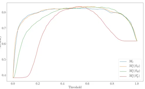
Evaluation. Figures 5a and 5b and Table 4 show the results of the conducted evaluation for the five effect prediction models. Figures 5a and 5b visualise the impact on accuracy and recall with different thresholds on the M2-M2? predic-tion scores, while Table 4 presents the relevant evaluapredic-tion metrics with a thresh-old of 0.5 forM2-M2?and 30 neighbours forM1. The results can be summarised as follows:
(i) M1 is only slightly better than random choice, as the prior binary output distribution is 0.59 and 0.41. Thus it would not be appropriate for predict-ing effects. The false positive rate is also high, hence, M1 would not be practical to use as a recommendation system.
(ii) M2 is considerably better thanM1 and has balance between precision and recall. We suspect that this balance is due to random choice when the model has not previously seen a chemical or species.i.e., a prediction close to the decision boundary when an input is unseen will maintain the false negative/positive proportion, hence good for accuracy, not necessary for giving (interesting) recommendations to the laboratory.
(iii) Introducing the background knowledge to M2, in the form of KG embed-dings gives higher recall, without loosing accuracy. In contrast toM2,M2? is more uncertain when unseen combinations are presented to the model (in dubio pro reo). Therefore,M2? is better suited to giving recommenda-tions for cases where there is limited information about the chemical and the species in the effect data.
(iv) The best results in terms of recall, when using a threshold of 0.5 (see Ta-ble 4), are obtained byM?
2 with the embeddings provided by HolE (9 points higher than theM2).
(a) Accuracy for theM2 andM2?prediction models.
[image:15.612.183.431.132.284.2](b) Recall for theM2 andM2?prediction models.
Fig. 5: Accuracy and Recall for theM2andM2? models with various thresholds.
the accuracy. TransE and HolE-based models have higher recall (0.97 and 0.94) at decision threshold 0.30, however, this comes at a cost of reduction in accuracy (0.74 and 0.79).
7
Discussion and future work
We have created a knowledge graph called TERA that aims at covering the knowledge and data relevant to the ecotoxicological domain. We have also imple-mented a proof-of-concept prototype for ecotoxicological effect prediction based on knowledge graph embeddings. The obtained results are encouraging, showing the positive impact of using knowledge graph embedding models and the benefits of having an integrated view of the different knowledge and data sources.
Knowledge graph.The TERA knowledge graph is by itself an important con-tribution to NIVA. TERA integrates different knowledge and data sources and aims at providing an unified view of the information relevant to the ecotoxicol-ogy and risk assessment domain. At the same time the adoption of a RDF-based knowledge graph enables the use of (i) an extensive range of Semantic Web infrastructure that is currently available (e.g., reasoning engines, ontology align-ment systems, SPARQL query engines), and(ii)state of the art knowledge graph embedding strategies.
Prediction models.The obtained predictions are promising and show the va-lidity of the selected models in our setting and the benefits of using the TERA knowledge graph. As mentioned before, we favour recall with respect to precision. One the one hand, false positives are not necessarily harmful, while overlooking the hazard of a chemical may have important consequences. On the other hand, due to the limited experiments in terms of concentration (i.e., effect data may not be complete), some chemicals may look less toxic than others while they may still be hazardous.
Value for NIVA. The conducted work falls into one of the main research lines of NIVA’s Computational Toxicology Program (NCTP) to enhance the generation of hypothesis to be tested in the laboratory [15]. Furthermore, the data integration efforts and the construction of the TERA knowledge graph also goes in line with the vision of NIVA’s section for Environmental Data Science. The availability and accessibility of the best knowledge and data will enable optimal decision making.
Novelty.Knowledge graph embedding models have been applied in general pur-pose link discovery and knowledge graph completion tasks [22]. They have also attracted the attention in the biomedical domain to find, for example, candi-date genes for a disease, protein-protein interactions or drug-target interactions (e.g., [3, 2]). However, we are not aware of the application of knowledge graph embedding models in the context of toxicological effect prediction.
in-teractions) and compounds (e.g., target proteins) which is expected to enhance the computed embeddings and the effect predictions.
Resources. The datasets, evaluation results, documentation and source codes are available from the following GitHub repository: https://github.com/Erik-BM/NIVAUC
Acknowledgements
This work is supported by the grant 272414 from the Research Council of Nor-way (RCN), the MixRisk project (RCN 268294), the AIDA project, The Alan Turing Institute under the EPSRC grant EP/N510129/1, the SIRIUS Centre for Scalable Data Access (RCN 237889), the Royal Society, EPSRC projects DBOnto, MaSI3 and ED3. We would also like to thank Martin Giese and Zofia C. Rudjord for their contribution in early stages of this project.
References
1. Agibetov, A., Jim´enez-Ruiz, E., Ondresik, M., Solimando, A., Banerjee, I., Guer-rini, G., Catalano, C.E., Oliveira, J.M., Patan`e, G., Reis, R.L., Spagnuolo, M.: Supporting shared hypothesis testing in the biomedical domain. J. Biomedical Se-mantics9(1), 9:1–9:22 (2018)
2. Agibetov, A., Samwald, M.: Global and local evaluation of link prediction tasks with neural embeddings. In: 4th Workshop on Semantic Deep Learning (ISWC workshop). pp. 89–102 (2018)
3. Alshahrani, M., Khan, M.A., Maddouri, O., Kinjo, A.R., Queralt-Rosinach, N., Hoehndorf, R.: Neuro-symbolic representation learning on biological knowledge graphs. Bioinformatics33(17), 2723–2730 (2017)
4. Arnaout, H., Elbassuoni, S.: Effective Searching of RDF Knowledge Graphs. Web Semantics: Science, Services and Agents on the World Wide Web48(0) (2018) 5. Bordes, A., Usunier, N., Garcia-Duran, A., Weston, J., Yakhnenko, O.: Translating
embeddings for modeling multi-relational data. In: Advances in Neural Information Processing Systems 26, pp. 2787–2795. Curran Associates, Inc. (2013)
6. ChEBI-ontology: The european bioinformatics institute (2019), https://www.ebi.ac.uk/chebi/
7. Chollet, F., et al.: Keras. https://github.com/fchollet/keras (2015)
8. Duchi, J., Hazan, E., Singer, Y.: Adaptive subgradient methods for online learning and stochastic optimization. J. Mach. Learn. Res.12, 2121–2159 (Jul 2011)
9. EPA, U.: Ecotoxicology knowledgebase (ecotox) (2019),
https://cfpub.epa.gov/ecotox/
10. Euzenat, J., Shvaiko, P.: Ontology Matching, Second Edition. Springer (2013) 11. Jim´enez-Ruiz, E., Cuenca Grau, B.: LogMap: Logic-Based and Scalable Ontology
Matching. In: 10th International Semantic Web Conference. pp. 273–288 (2011) 12. Jimenez-Ruiz, E., Cuenca Grau, B., Zhou, Y., Horrocks, I.: Large-scale
interac-tive ontology matching: Algorithms and implementation. In: the 20th European Conference on Artificial Intelligence (ECAI). pp. 444–449. IOS Press (2012) 13. Kadlec, R., Bajgar, O., Kleindienst, J.: Knowledge base completion: Baselines
14. Lehmann, J., Isele, R., Jakob, M., Jentzsch, A., Kontokostas, D., Mendes, P.N., Hellmann, S., Morsey, M., van Kleef, P., Auer, S., Bizer, C.: DBpedia - A large-scale, multilingual knowledge base extracted from Wikipedia. Semantic Web6(2), 167–195 (2015)
15. Myklebust, E.B., Jimenez-Ruiz, E., Rudjord, Z.C., Wolf, R., Tollefsen, K.E.: In-tegrating semantic technologies in environmental risk assessment: A vision. In: 29th Annual Meeting of the Society of Environmental Toxicology and Chemistry (SETAC) (2019)
16. NCBI-Taxonomy: The national center for biotechnology information (2019), https://www.ncbi.nlm.nih.gov/taxonomy
17. Nickel, M., Rosasco, L., Poggio, T.A.: Holographic embeddings of knowledge graphs. CoRRabs/1510.04935(2015), http://arxiv.org/abs/1510.04935 18. Nikolova, N., Jaworska, J.: Approaches to measure chemical similarity a review.
QSAR & Combinatorial Science22(910), 1006–1026 (2003)
19. Pradeep, P., Povinelli, R.J., White, S., Merrill, S.J.: An ensemble model of QSAR tools for regulatory risk assessment. Journal of cheminformatics8, 48–48 (2016)
20. PubChem: National institutes of health (nih) (2019),
https://pubchem.ncbi.nlm.nih.gov/
21. Vrandecic, D., Kr¨otzsch, M.: Wikidata: a free collaborative knowledgebase. Com-mun. ACM57(10), 78–85 (2014)
22. Wang, Q., Mao, Z., Wang, B., Guo, L.: Knowledge graph embedding: A survey of approaches and applications. IEEE Trans. Knowl. Data Eng. 29(12), 2724–2743 (2017)