Direct Solution of Multi-Objective Optimal Control Problems
Applied to Spaceplane Mission Design
Lorenzo A. Ricciardi∗, Christie Alisa Maddock†and Massimiliano Vasile‡ University of Strathclyde, Glasgow, United Kingdom, G1 1XJ
This paper presents a novel approach to the solution of multi-phase multi-objective optimal
control problems. The proposed solution strategy is based on the transcription of the optimal
control problem with Finite Elements in Time and the solution of the resulting Multi-Objective
Non-Linear Programming (MONLP) problem with a memetic strategy that extends the Multi
Agent Collaborative Search algorithm. The MONLP problem is reformulated as two non-linear
programming problems: a bi-level and a single level problem. The bi-level formulation is used
to globally explore the search space and generate a well spread set of non-dominated decision
vectors while the single level formulation is used to locally converge to Pareto efficient solutions.
Within the bi-level formulation, the outer level selects trial decision vectors that satisfy an
improvement condition based on Chebyshev weighted norm, while the inner level restores
the feasibility of the trial vectors generated by the outer level. The single level refinement
implements a Pascoletti-Serafini scalarisation of the MONLP problem to optimise the objectives
while satisfying the constraints. The approach is applied to the solution of three test cases
of increasing complexity: an atmospheric re-entry problem, an ascent and abort trajectory
scenario and a three-objective system and trajectory optimisation problem for spaceplanes.
Nomenclature
b = static parameter vector
C = constraint vector CD = drag coefficient CL = lift coefficient
D = aerodynamic drag force (N) E = energy function
fs,j = Bernstein polynomials
∗
Ph.D. Candidate, Aerospace Centre of Excellence, Mechanical & Aerospace Engineering, 75 Montrose Street, G1 1XJ, Glasgow, AIAA Student Member.
†
Lecturer, Aerospace Centre of Excellence, Mechanical & Aerospace Engineering, 75 Montrose Street, G1 1XJ, Glasgow, AIAA Member.
‡
g = algebraic constraints
g0 = magnitude of gravitational acceleration at sea level (m/s2) h = altitude (m)
Is p = specific impulse (s)
J = objective vector
L = aerodynamic lift force (N)
M = mach number
m = vehicle mass (kg) mp = mass of propellant (kg)
p = decision vector
pa = atmospheric pressure (Pa) qflux = heat flux (W/m2)
RE = radius of the Earth (m)
r = position vector in inertial frame (m) Sr e f = aerodynamic surface reference area (m2)
T = time domain
T = magnitude of thrust (N)
t = time (s)
u = control vector
v = velocity in inertial frame (m/s)
w = weight functions
x = state vector
y = vector of state weights
z = utopia point
α = angle of attack (rad) βk = Gauss integration weights γ = flight path angle (rad) δT = throttle
θ = latitude (rad) λ = longitude (rad)
σ = bank angle (rad) τ = normalised time φi = scalar objective function
χ = heading angle (rad)
ψ = boundary constraints ω = weight of descent directions
ωE = magnitude of angular velocity of the Earth (rad/s) Subscripts
0 = initial
f = final
I. Introduction
T
his paper proposes a method for the solution of multi-objective, multi-phase optimal control problems. In the pastthree decades, a considerable body of work has been dedicated to the direct solution of single objective optimal control problems, see e.g., [1–8] and references therein, and translated into a number of commercial and open source software∗,†. However, while conditions of optimality and related theoretical aspects of multi-objective optimal control problems have been studied in a number of papers, see [9–13] and references therein, less research has been dedicated to the solution of multi-objective optimal control problems.Ober-Blöbaum et al. [14] coupled a direct transcription approach with an approach that scalarised the multi-objective vector along directions pointing at predefined unreachable points in the criteria space. Each scalar problem was then solved with a standard NLP solver. This approach was employed to solve an interplanetary trajectory optimisation. Kaya and Maurer [15] proposed a similar approach but used the Pascoletti-Serafini scalarisation [16] to transform the multi-objective optimisation problem in a set of single-objective optimisation problems, and employed the resulting approach to solve chemical reaction engineering and drug dosage problems. Pagano and Mooij [17] optimised the mass of the payload for a launch vehicle and minimised the violation of the constraints as a second objective, Bairstow et al. [18] performed a multiobjective optimisation of a two stage launcher minimising cost and maximising the payload and Roshanian et al. [19] performed robust design optimisation of a two stage launch vehicle by means of multiobjective optimisation, minimising both the mean and the variance of the gross take-off mass when several design and operative parameters where subject to uncertainty. In these last three works the control laws had a simple parametric shape. The parameters describing those shapes were optimisation variables, and stochastic multiobjective optimisation algorithms were employed to find the set of Pareto optimal solutions. Coverstone-Carroll et al. [20] combined Genetic Algorithms
and optimal control theory in a dual loop algorithm. In the outer loop, a Multi-Objective Genetic Algorithm (MOGA) was generating vectors of co-states and times of flight. For each set, the inner loop was solving a single objective optimal control problem with given time of flight, minimising the propellant consumption. Englander et al. [21] proposed a dual loop algorithm in which the outer loop solves a multi-objective problem handling a set of categorical variables through a multi-objective genetic algorithm and the inner loop solves a set of single objective constrained optimal control problems using Monotonic Basin Hopping [22].
The method proposed in this work is based on a direct transcription with Finite Elements in Time [6] (DFET) and a solution of the resulting Multi-Objective Nonlinear Programming (MONLP) problem with a version of Multi Agent Collaborative Search [23] (MACS) called MACSoc. DFET have been successfully used to solve many difficult single-objective trajectory optimisation problems [3, 4, 24, 25]. Similarly, MACS has been tested and validated on a number of benchmarks of difficult multi-objective optimisation problems[23][26]. Previous work by the authors validated the pairing of DFET and MACS on a set of optimal control problems with known solutions [27][28]. Here, this pairing is extended to treat more complex multi-objective optimal control problems, with the inclusion of static system design parameters and multiple phases. The method proposed in this paper differentiates from Ober-Blöbaum et al. [14] and Kaya and Maurer [15] in that it combines a global exploration and local convergence with a smooth transition between Chebyshev and Pascoletti-Serafini scalarisation [16] and incorporates an automatic and unsupervised procedure to generate feasible first guesses. It also differentiates from [17–21] in that it does not use a generic MOGA but proposes a more efficient memetic approach and implements a more general direct transcription method.
The method is applied to three realistic test cases for spaceplane-based launch vehicles, optimising the ascent, descent and abort trajectories and some key vehicle and mission design variables. A considerable amount of work has been devoted to the off-line optimisation of ascent and re-entry trajectories for launch systems with the inclusion of progressively more sophisticated physics and constraints examining the launch system design and performance [29–33], and the fast and robust generation of a guidance law with the ultimate goal to have an on-line closed loop guidance update [34–39]. This paper departs from these two streams of research, and focuses on the off-line generation of Pareto optimal trade-off solutions for a generic multi-objective optimal control problem. The three test cases were selected to show the benefits of this method to the trade-off and feasibility studies conducted during the initial design phases.
II. Direct Transcription of Multi-Objective Optimal Control Problems
Multi-, or more generally many, objective optimal control problems can be formulated as follows:
min
u∈U,b∈BJ s.t.
Û
x=F(x,u,b,t)
g(x,u,b,t) ≥0 ψ(x0,xf,t0,tf,b) ≥0
t ∈ [t0,tf]
(1)
where J = [J1,J2, ...,Ji...,Jm]T is, in general, a vector of objectives Ji that are functions of the state vectorx :
[t0,tf] →Rn
, control variablesu ∈ L∞(U ⊆Rnu), static parametersb ∈ B ⊆Rnb and timet. The functionsx(t) belong to the Sobolev spaceW1,∞while the objective functions are Ji :R3n+2×Rnu ×Rnb −→R. The objective vector is subject to a set of dynamic constraints withF : Rn×Rnu ×Rnb × [t0,tf] −→Rn, algebraic constraints
g:Rn×Rnu ×
Rnb × [t0,tf] −→R ng
, and boundary conditionsψ:R2n+2×Rnb −→Rnψ. In the following we will consider only Mayer’s types of optimal control problems, whereby each objective function is expressed as a scalar function of the boundary conditions, boundary times and static parameters:
Ji =φ(x0,xf,t0,tf,b) (2)
Note that, if boundary states and times, x0,xf,t0,tf are free decision variables, they can be included in the static parameter vectorband the union of controls and static parameters is called a decision vector. Thus, without loss of generality, one can say that the solution of problem (1) is a subset ofU×Bthat satisfies the constraints and contains Pareto efficient decision vectors. This leads to the following definition.
Definition II.1 Given the subsetΩU ⊂U×Bof feasible decision vectors, a decision vector[u∗,b∗] ∈ΩU is said to be Pareto efficient if[u∗,b∗][u,b],∀[u,b] ∈ΩU.
The symbol of dominanceis introduced to indicate that if[u,b]1 [u,b]2thenJi([u,b]2) ≤Ji([u,b]1)fori=1, . . . ,m and∃jsuch thatJj([u,b]2)<Jj([u,b]1).
A. Direct Transcription with Finite Elements in Time
transcribe the differential equations into a set of algebraic equations. Finite Elements in Time (FET) for the indirect solution of optimal control problems were initially proposed by Hodges and Bless [40], and during the late 1990s evolved to the discontinuous version. As pointed out by Bottasso and Ragazzi [41], FET for the forward integration of ordinary differential equations are equivalent to some classes of implicit Runge-Kutta integration schemes, can be extended to arbitrary high-order, are very robust and allow full h-p adaptivity. In the past decade, direct transcription with FET on spectral bases has been successfully used to solve a range of difficult problems: from the design of low-thrust multi-gravity assist trajectories to Mercury [4] and to the Sun [25], to the design of weak stability boundary transfers to the Moon, low-thrust transfers in the restricted three body problem and optimal landing trajectories to the Moon [24]. Following the standard procedure for DFET transcription (see [6] for more details), the time domainTis decomposed intoNfinite elements such that:
T =
N
Ø
j=1
Tj(tj−1,tj)=
t0,tf
(3)
withtN =tf. On each time element, the differential constraints in (1) are first recast in weak form and integrated by parts leading to:
∫
Tj Û
wTx+wTF(x,u,b,t)dt−wT(tj)xbj +wT(tj−1)xbj−1=0 (4)
whereware generalised weight functions, andxbj andx b
j−1are the values of the states at the boundaries of each element.
Then, states, controls and weight functions are transcribed in polynomial form as follows:
xj(t)= lx Õ
s=0
fs,j(t)xs,j (5a)
uj(t)= lu Õ
s=0
fs,j(t)us,j (5b)
wj(t)= lx+1
Õ
s=0
fs,j(t)ws,j (5c)
where functions fs,j are chosen among the space of Bernstein polynomials. It is practical to redefine Eq. (4) and basis functions (5) over the normalised interval[−1,1]through the transformation:
τ=2
t−tj−tj−1 2 tj−tj−1
tj−1 ≤t ≤tj (6)
whereτis the normalised time. This way the domain of the basis function is constant and irrespective of the size of the element. By substituting Eqs. (5) into (4) and solving the integral with a Gauss quadrature formula onluGauss nodes, one gets:
lu Õ
k=0 βk
Û
wj(τk)Txj(τk)+wj(τk)TFj(τk) ∆tj
2
−wT(1)xbj +wT(−1)xbj−
whereτkandβkare Gauss nodes and weights,∆tj =(tj−tj−1)andFj(τk)is the shorthand notation forF xj(τk),uj(τk),b,t(τk). Since Eq. (7) must be valid for every arbitraryws,j, Eq. (7) gives rise to a system of(lx+1)vector equations for each element:
Ílu
k=0βk
h Û
f1,j(τk)xj(τk)+f1,j(τk)Fj(τk)
∆tj
2
i
+xbj−
1=0 ..
.
Ílu
k=0βk
h Û
fs,j(τk)xj(τk)+fs,j(τk)Fj(τk)
∆tj
2
i
=0 ..
.
Ílu
k=0βk
h Û
flx+1,j(τk)xj(τk)+ flx+1,j(τk)Fj(τk)
∆tj
2
i
−xbj =0
(8)
Path constraints are evaluated at Gauss nodes for each element:
g xj(τk),uj(τk),b,t(τk) ≥0 (9)
Continuity conditions are then imposed on the boundary states of adjacent elements, such that all boundary valuesxbj cancel out except for the initial boundary term of the first elementxb0 and last boundary element of the last elementxbf. Thus, once all the elements are assembled together, the only parameters (or decision variables) that remain to be defined arexs,jfor the states,us,j for the controls, the boundary statesxb0 andxbf, the time variablest0 andtf and the static parametersb. Each transcribed objective function in Mayer’s form (2) is calculated simply as:
˜
Ji=φi(xb0,xbf,t0,tf,b) (10)
The time domainTcorresponds to a single time phase, or timeline. However, a general problem can have multiple phases either in series or in parallel. For example, a multi-stage vehicle can have one phase per vehicle stage with all phases connected in series for the ascent, and/or branching parallel phases for the upper stage ascent and first stage descent and return. These branching phases can also be seen in abort scenarios, which comprises one of the test cases in this paper. WhenNpphases are present, dynamic constraints (7), path and boundary constraints,gandψ, and objective functions (10) are defined on each timeline. In order to connect different timelines, a set ofNi pinter-phase constraints are introduced:
ψsp
xb
0,Is p,x
b
f,Is p,t0,Is p,tf,Is p
≥0 sp=1, ...,Ni p (11)
where the index vectorIsp collects all the indexes of the phases that are connected by constraintψsp. Note that the
number of phases is fixed, but their temporal order is actually defined by the inter-phase constraints (11). Section IV will show one example with two sequential phases and another one with branching parallel phases.
constraints (11), can be written, in vector form, as:
min
y∈Y,p∈Π˜J
s.t.
C(y,p) ≥0
(12)
wherey=[x0,1, ..,xs,j, ...,xlx,N]
T
,Yis a box inRnY withnY =n(lx+1)N,p=[u0,1, ..,us,j, ...,ulu,N,b ∗]T
collects all the static and discretised dynamic control variables,b∗ =[b,xb0,xbf,t0,tf]T,Π⊆Rns ×
Rn ∗
b, withns =nu(lu+1)N
(assuming that each element has the same number of control parameters) andn∗b =nb+2n+2, andCcollects all constraints, including boundary and interphase ones.
Similar to problem (1), the solution of problem (12) is a subset ofΩΠ ⊂Πthat satisfies the constraints and contains vectorspthat are Pareto efficient. For continuous functions, the subsetΩΠ is a manifold inRns+n
∗
b with dimension ≤ (m−1)[42]. In the following, the goal will be to identify a pre-defined countable number of Pareto efficient solutions
contained inΩΠ.
III. Solution of the Transcribed Problem
Problem (12) is solved with a memetic many-objective optimisation algorithm, adapted from MACS (Multi-Agent Collaborative Search [23, 26]) and called MACSoc, that combines a stochastic agent-based global search with a local (gradient-based in this case) refinement of the solutions [27, 28, 43]. The overall solution process implemented in MACSoc is summarised in Algorithm 1.
At the start of MACSoc,Nacandidate solutions are generated with a Latin Hypercube sampling, associated to a populationP0ofNaagents, and an attempt is made to make each candidate solution feasible before the optimisation process starts (line 1 in Algorithm 1). Both the global search and local refinement strategies implemented in MACSoc require the definition of a set of descent directions in criteria space, thus, after initialising the agents, the algorithm generatesNwuniformly spread weight vectorsω(line 2 in Algorithm 1) that define the components ofNwdescent vectors; this is explained further in Subsection E. Each agent will be associated to a different weight vector, allowing each agent to converge to a different part of the Pareto front.
Algorithm 1MACS optimal control (MACSoc) framework 1: Initialise populationP0and global archiveA0,k=0,ρB=1
2: Initialise weight vectorsω
3: whilen_f un_eval<max_f un_evaldo
4: Run individualistic heuristics onPk using bi-level formulation
5: Pk → Pk+
6: Update archiveAk with potential field filter
7: Run social heuristics combiningPk+andAk using bilevel formulation
8: Update archiveAk with potential field filter
9: Pk+→ Pk†
10: iflocal search triggeredthen
11: Run gradient based refinement using single level formulation
12: Pk† → Pk∗
13: Update archiveAk with potential field filter
14: Pk∗→ Pk+1
15: else
16: Pk† → Pk+1
17: end if
18: k=k+1
19: UpdateρB 20: end while
archiveAk (lines 5, 6, 8, 9 and 13 in Algorithm 1). After every user specified number of iterations, and as a last step before the algorithm ends, the local refinement is triggered, and the archive and population are updated with the refined solutions (lines 10 to 17 in Algorithm 1). The local refinement solves a single level scalarised version of problem (12). The process proceeds alternating social and individualistic actions, with periodic local refinement, until a maximum number of calls to the objective vectormax_fun_evalis reached. The overall algorithmic complexity is dominated by the NLP solver used in the bi-level problem and for the local refinement.
In the following both the bi-level and single level problems are explained in more detail together with the heuristics used to generate new candidate solutions. Note that the combined use of the bi-level formulation, for global exploration, and single level formulation for local convergence, within MACSoc is one of the distinctive features of the proposed approach compared to previous works such as [14], [15] and [21].
A. Bi-level Global Optimisation Problem
The global search part of the algorithm solves the following two-level problem:
min
p∗ ˜J(y ∗,p∗)
s.t.
(y∗,p∗)=
argmin(y,p) δ
p(y,p) |C(y,p) ≥0
Problem (13) defines two different optimisation sub-problems at two different levels. The outer level handles the objective vector˜Jand generates tentative decision vectorsp. Tentative solutions are then submitted to the inner level, whose goal is to find the state and control vectorsy∗andp∗that satisfy constraintsCand minimise an inner cost function δp=kp∗−pk. Thus, the inner level will look for the closest feasible solution to the tentative one generated by the outer level. The outer level then receives the solution(y∗,p∗)and proceeds by evaluating the objective functions associated to
p∗. The inner level problem is solved with a generic NLP solver (Matlabfminconin this case).
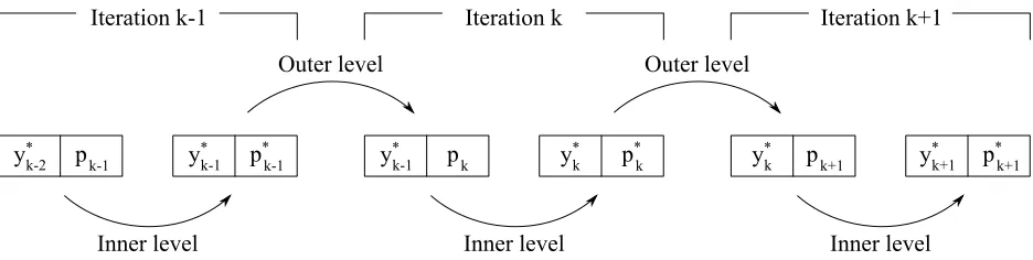
In order to reduce the number of iterations required by the inner level to converge, the outer level stores the feasible statesy∗at iterationkto be used as a warm start for the inner level at iterationk+1. As illustrated in Fig. 1, the feasible statesy∗k are preserved from iterationkto iteration(k+1)and the outer level only generates a new tentative vectorpk+1. The inner level at iteration(k+1)will thus usey∗k andpk+1as initial guesses for states and controls. Because of the waypk+1is generated, even ify
∗
k is associated top
∗
k, it works well as an initial guess also when associated topk+1. When individualistic actions are applied, each agent generates one or more tentative vectors through three mechanisms that are triggered one after the other in this order: Inertia→Pattern Search→Differential Evolution. If any of these mechanisms produces an improved solution, the following ones are not triggered and the process proceeds by updating the population and archive (line 5 and 6 of Algorithm 1). The three mechanisms operate as follows:
• Inertiais triggered by agentjonly if, in the previous iteration, agentjgenerated an improved solution. In this case a step with random length is taken in the direction defined by the vectorp∗k−p∗k−1.
• Pattern Searchconsists of changing one optimisation parameter at a time by a random amount in each direction within a given neighbourhoodBj of agent j. The order by which the parameters are changed is a random permutation of the number of decision parameters. The process is repeated until either an improvement is registered or the maximum number of trials has been reached. As in [23], the maximum number of trials is dynamically adjusted during the optimisation process: when the Archive is empty, the maximum number of parameters scanned is equal to the total number of optimisaton parameters. This maximum value is decreased linearly as the Archive fills up, until only one optimisation parameter is changed when the Archive is full. The neighbourhoodBjis a box centred in the position of the agent in parameter space and with the edges equal to the edges of the search spaceΠmultiplied by the scaling parameterρBj.
• Differential Evolutiongenerates a sample with the simple heuristic:
ptr ial,j =pj+ξ1e pj−pj1 +
cF pj2−pj3 (14)
wherepj is the current solution,pj1,pj2,pj3 are three randomly chosen solutions from the current population
Inner level Inner level Inner level
Outer level Outer level
Iteration k-1 Iteration k Iteration k+1
y*
k-2 pk-1 y
*
k-1 pk y
* k
p*k-1 y*
k-1 p
*
k y
*
k pk+1 y
*
k+1 p
* k+1
Fig. 1 Schematic representation of the bilevel approach acting on a single solution.
constructed as follows:
ej =
1, ifξ2<C R 0, otherwise
(15)
whereξ2 is another uniformly distributed random number in the unit interval andC Ris a constant, known as crossover rate. In this work,cF=0.9 andC R=1.
If no improvement is made after trying all the three heuristics,ρBis halved, while if an improvement is made, it is doubled until the initial valueρB=1 is reached again.
When social actions are applied, the outer level uses the entire populations of agents to generate a tentative solution using heuristic (14), but the parent solutionspj1,pj2,pj3 are chosen from the union of the current populationPkand the current archiveAk.
A candidate solution(y∗,p∗), generated by the inner level, is evaluated, in the outer level, by computing the weighted Chebychev norm:
Φi =max i ωi
˜
Ji(y∗,p∗) −zi (16)
whereωiare the components of a weight vector in objective space andzi =minPk∪AkJ˜i are the components of the
current utopia point, or the point whose coordinates are the minimum value of each objective function ˜Jiover all the elements of the population and the archive combined. Norm (16) measures the distance, along each coordinate in objective space, between the current objective vector ˜J(y∗,p∗)and the current utopia pointz, weights the different distances viaω, and takes the worst, or maximum, weighted distance. Therefore, given the value ofΦiat stepk, orΦki, an improvement corresponds toΦik+1 <Φki. This improvement criterion has two very important properties: first, it allows one to reach even non-convex parts of the Pareto front, and second, if the weights are chosen appropriately, it allows one to efficiently converge to the minimum possible values of each objective function. The generation of the weightsωwill be explained in Subsection E.
[image:11.612.73.541.68.186.2]the archive and population. This creates an adaptive rejection mechanism: if none of the agents are feasible, the ones that best satisfies the feasibility is temporarily entered in the archive with the next iterations trying to further improve their feasibility. Once an agent finds a feasible solution, it will explore the search space through the global bi-level approach, generating several feasible and non dominated solutions. These solutions will enter in the archive because they will dominate many of the existing non-feasible ones, and thanks to the social actions some agents will be directly moved onto those solutions, allowing the whole population to converge to feasible solutions in a handful of iterations. Finally if any tentative vector foryandpis outside the boundaries of the search spaceY ×Π, the vector is shrunk till it is back into the search space (for more details please refer to [23]).
B. Single Level Local Search
The local refinement solves the following scalarised problem for each agent j:
min
≥0
s.t.
ωi,jϑi,j(y,p) ≤ fori=1, . . . ,m
C(y,p) ≥0
(17)
whereωj is a vector of weights,ϑi,j is theithcomponent of the rescaled objective vector of the jth agent, and is a slack variable. This reformulation of the problem, known as Pascoletti-Serafini scalarisation [16], is constraining the agent’s movement, in criteria space, within the descent cone defined by the point(dj+ζj)along the direction
dj =(1/ω1,j, . . . ,1/ωi,j, . . . ,1/ωm,j). The rescaled objective vector is defined as:
ϑj(y,p)= ˜
Ji,j(y,p) −zi˜ z∗i,j−z˜i for
i=1, . . . ,m (18)
wherez∗j is equal to ˜Jj(y,p),(y,p)is the initial guess for the solution of (17) and ˜z=z−zAwithzAthe nadir of the archive, or point whose components are the maximum values of all the components of the objective vectors in the archive. From the normalisation one can derive the components of the vectorζj:
ζi,j = zi
z∗i,j−zi˜ fori=1, . . . ,m (19)
important to remark that Problem (16) and (17) are equivalent and lead to the same optimal solution if the target point for the Pascoletti-Serafini scalarisation coincides with the utopia point and the weight vectors are the same. As such, the following theorem holds true [44]:
Theorem III.1 A point(,y,p) ∈ R×Y ×Π is a minimal solution of (17)withz∈ Rm,zj < miny∈Y,p∈ΠJj(y,p), j=1, . . . ,m, andω∈int(Rm+)if and only ifyandpare a solution of (16).
Therefore, by combining (16) in the global search phase with (17) in the refinement phase, the algorithm realises a smooth transition from global exploration of the Pareto set, to local convergence.
C. Archiving Strategy
MACS employs a unique archiving strategy proposed by Ricciardi and Vasile in [23] that is also applied in the context of MACSoc. When the elements in the archiveAare less than the maximum allowed cardinality ofA, every new feasible and non-dominated solution is stored in the archive. Once the maximum size is reached, a retention-rejection policy is implemented. The retention-rejection policy is based on a minimum energy principle. New elements are added toAonly if they minimise the potential function:
E J˜1,· · ·,J˜NA =
NA Õ
i=1 NA Õ
j=i+1
1
(J˜i−J˜j)T(J˜i−J˜j)
(20)
whereNAis the number of elements inA. To avoid biasing the in the rejection-retention process when the objectives have different scales, the objective values of the set of non dominated solutions are all normalised between 0 and 1. This leads to a combinatorial problem that can be solved approximately but efficiently using the approach described by Ricciardi and Vasile [23], and returns a uniformly spread set of points. This minimum energy criterion is also used for the generation of uniform descent directions, as will be explained in Subsection E.
D. Generation of the Initial Feasible Population
Before the optimisation starts, MACSoc generates an initial population of agentsP0(see line 1 of Algorithm 1) with the following four-step automatic and unsupervised procedure:
1) A first guess for the decision vectors is generated with a Latin Hypercube sampling within the prescribed boundaries. State variables for each phase are initialised with a simple linear interpolation between initial and final conditions.
2) For each phase, each integral equation (7) is made feasible by solving only the inner level subproblem of problem (13) with an NLP solver.
4) All phases are connected together and the inter-phase constraints are satisfied applying again the same NLP solver to the subproblem in (13).
If, at the end of the initialisation phase, an agent is associated to a solution that is not feasible within the prescribed tolerance, that solution is still included in the initial populationP0and submitted to the subsequent optimisation cycle. In the following, the feasibility level required to the initial population is the same required for the rest of the algorithm, which is 10−6, so if the NLP converges, the solution generated by this approach is a fully feasible solution. By default, the NLP solver is allowed to use a maximum number of calls to the constraint function that is equal to 10(n∗b+ns+nY). For this procedure, an Interior Point NLP algorithm was used because it delivered a more robust and consistent convergence to feasible solutions.
E. Definition of the descent directions and target points
The weight vectors for the bi-level global search are generated as follows: first, a simplex in objective space is generated through simplex lattice design [45]. Then, the points of this simplex lattice are projected on the unit sphere by dividing their position vectors by their distance to the origin. This gives a fairly uniform distribution of weight vectors (and thus descent directions) in anyNwdimensional space. In order to generate a more uniform distribution, however, these weight vectors are used as an initial guess for the following optimisation problem:
min E(ω1, . . . ,ωNw)
s.t.
ωT iωi=1
(21)
whereE(ω1,· · ·,ωNw)is calculated using Eq. (20). This optimisation problem can be quickly solved with a standard
NLP solver. As a reference, from the initial lattice to the final optimised distribution the generation of 106 uniformly spread weight vectors for the three objective problem in Section C takes 22 iterations of the NLP solver with an SQP algorithm, which translates into approximately half a second in Matlab on an i7 laptop. While this approach is valid for generalm-objective problems, for two objective problems it is simpler and faster to generate uniformly angularly spaced weight vectors. In the followingNa=Nw and each agent is associated to the closest descent direction in criteria space, at the initialisation stage, with the constraint that no two agents can have the same descent direction.
For the single level approach, the weight vectorsωj =[
√
2, . . . ,
√
orthogonal weight is associated to jand problem (17) is solved with the added constraints:
˜
Ji ≤zi ∀i, j (22)
The reason for the different choice of weight vectors between the bi-level and the single level formulation can be explained as follows: the bi-level formulation explores globally the search space with a population of agents, thus there is the need to maximise the spreading of the solutions, on the contrary, the single-level is used to improve the local convergence of each agent in a normalised criteria space. Thus the goal of the single level is to return dominating solutions without altering too much their spreading in criteria space.
IV. Case Studies
The approach to the solution of multi-objective optimal control problems described in previous sections is applied to three problems of increasing complexity: a known re-entry benchmark problem with 2 objectives, a 2 phase ascent problem with 3 objectives, and 3 phase branched ascent and abort problem with 2 objectives. The code and all the test cases in this paper were implemented in Matlab 2017b and run on a laptop with an i7 processor under Windows 10. The gradient based refinement was run every 10 iterations in all cases, and the NLP solver used in both the bi-level and single level formulations employed an SQP algorithm. The maximum number of calls to the constraint function for the NLP solver in the bi-level formulation was set equal ton∗b+ns+nY, while it was increased to 10(n∗b+ns+nY)in the single level refinement.
A. Physical models
1. Dynamical model
The vehicle dynamics are modelled as a 3DOF point mass moving in an Earth Centred Inertial reference frame (adapted from [5]),
Û
r =hÛ =vsinγ (23a)
Û
θ=v
r cosγcosχ (23b)
Û
λ= v
rcosθcosγsinχ (23c)
Û
v=T(δT)cosα−D
m −gsinγ (23d)
Û
γ=T(δT)sinα+L
mv cosσ+
v
r −
g v
cosγ (23e)
Û
χ=T(δT)sinα+L mvcosγ sinσ+
v
rcosθcosγsinχsinθ (23f)
Û
m=− Ûmp(δT) (23g)
wherer =krkis the modulus of the position vectorr,h=r−RE is the altitude,λandθare longitude and latitude,
v=kvkis the magnitude of velocity vector,γand χare the flight path and heading angles,mis the mass of the vehicle, LandDare the aerodynamic lift and drag forces,g=µE/r2is the gravitational acceleration,Tis the thrust produced by the engine andmÛpis the propellent mass flow rate. The control variables are the angle of attackα, bank angleσ, and the throttlingδT of the engine.
2. Atmospheric and aerodynamic models
The International Standard Atmosphere model was used to model the atmospheric temperature, pressurepa, and densityρaas a function of the radiusrassuming a spherical Earth model with a radiusRE=6371 km and constant angular rotational velocityωE=7.292 118×10−5rad s−1. The atmosphere is assumed to rotate with the same angular velocity as the Earth, so the aerodynamic forces were computed using the velocity of the vehicle relative to the air with no wind (or other disturbances),
L =CLρaSr e fv 2 r el
2 (24)
D=CDρaSr e fv 2 r el
2 (25)
3. Propulsion model
The thrust vector is assumed to be always aligned with the vehicle longitudinal body axis and is proportional to the vacuum thrustTvacof the engine and modulated by the throttle controlδT ∈ [0, 1]. An additional term is added to account for the losses due to the difference between the nozzle’s exit pressure and the external atmospheric pressurepa. The resulting model is,
T =δT(Tvac−Aepa) (26)
whereAeis the nozzle exit area. The mass flow rate of the propellentmÛpis given by
Û
mp = δTTvac
Is pg0
(27)
whereIs pis the specific impulse of the engine andg0is the Earth gravitational acceleration at sea level.
B. Optimal Descent Trajectory
The first test case is based on a benchmark problem proposed by Betts [5] who analysed the unpowered re-entry of a Space Shuttle-like vehicle controlled by changing the angle of attackαand bank angleσ. To be consistent with Betts [5], the throttle was set toδT =0 for allt,ωE =0 and units are in the Imperial system. Furthermore, the following models and reference values were taken from Betts [5]: the exponential model for the atmosphere, the linear model for CL, the parabolic model forCD, the aerodynamic reference area ofSref=2690 ft2(249.9 m2) and the vehicle mass of 6309 sl (92 t). Bounds on the rate of change of the flight path and heading angles were imposed: | Ûγ| ≤0.035 rad s−1 and| Ûχ| ≤0.035 rad s−1s. A semi-empirical correlation for the heat flux at the nose was given as
qflux=
c0+c1α+c2α2+c 3α3
c4√ρa(c5v) c6 ≤
70 btu ft-2s-1 (28)
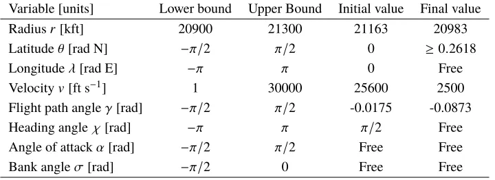
with the coefficientsc0,c1,c2,c3,c4,c5,c6as reported in [5]. Boundary conditions, lower bounds and upper bounds for the optimisation variables are listed in Table 1.
1. Objectives
Table 1 Lower bounds, upper bounds and boundary conditions for the Optimal Descent Trajectory case
Variable [units] Lower bound Upper Bound Initial value Final value
Radiusr[kft] 20900 21300 21163 20983
Latitudeθ[rad N] −π/2 π/2 0 ≥0.2618
Longitudeλ[rad E] −π π 0 Free
Velocityv[ft s−1] 1 30000 25600 2500
Flight path angleγ[rad] −π/2 π/2 -0.0175 -0.0873
Heading angle χ[rad] −π π π/2 Free
Angle of attackα[rad] −π/2 π/2 Free Free
Bank angleσ[rad] −π/2 0 Free Free
following single multi-objective optimisation problem:
min tf,u
[J1,J2]T = −θf,qu
T
s.t (29)
qf lux ≤qu
2. Numerical settings
The problem was formulated as a single time phase, with boundary conditions defined in Table 1, discretised using 6 finite elements and order 9 Bernstein polynomials for both states and controls, resulting in 121 optimisation parameters for the outer level (120 for the control variables, and 1 for the free final time), and 484 total variables for the single level and inner level NLP. A limit of 20000 calls to the objective vector was given to MACSoc, a population of 10 agents was deployed in the search space and the size of the archiveAwas limited to 10 elements. The initialisation of the population required approximately 1 second for 8 of the 10 agents, while for 2 agents it took approximately 3 minutes because the NLP solver did not converge to a feasible solution in the maximum number of iterations. However, as soon as the optimisation loop started, all solutions immediately became feasible thanks to the bi-level approach. The total runtime was approximately 1 hr.
3. Results
Fig. 2 Optimal descent trajectory: Pareto optimal solutions stored in the archiveAat the end of the optimisa-tion process and the two published single objective soluoptimisa-tions from Betts [5].
(a) (b)
Fig. 3 Optimal descent trajectory: time-history of a) the altitude and b) the velocity for each of the 10 solutions in the Pareto front in Fig. 2 plus the two published single objective solutions from Betts [5].
solutions from the reference are (−0.2618, 27.9982) and (−0.5345, 70) respectively. The relative difference in the second objectives is below 10−4 and can be attributed to the different NLP solvers and settings employed, and the presence of an iterative mesh refinement procedure in the reference solutions. In Figs. 3 and 5 the circles and squares represent the solutions from [5] for the two individual objective functions. The figures show a very good match between the result generated with MACSoc.
[image:19.612.191.418.72.241.2] [image:19.612.79.540.299.478.2](a) (b)
Fig. 4 Optimal descent trajectory: time-history of a) the lift to drag ratio and b) the heat flux for each of the 10 solutions in the Pareto front in Fig. 2.
(a) (b)
Fig. 5 Optimal descent trajectory: time-history of a) the angle of attack and b) the bank angle for each of the 10 solutions in the Pareto front in Fig. 2 plus the two published single objective solutions from Betts [5].
[image:20.612.80.538.78.261.2] [image:20.612.80.539.316.498.2](a) (b)
Fig. 6 Optimal descent trajectory: time-history of a) the rate of change of the flight path angleγÛ and b) the heading angle χÛfor each of the 10 solutions in the Pareto front in Fig. 2.
C. Three-objective Ascent Problem
This test case is the multi-objective, multidisciplinary design of a rocket-powered, two-stage launch vehicle optimised for the ascent to orbit. The vehicle is air dropped from a carrier aeroplane flying at 200 m s−1at an altitude of 10 km eastbound along the equator, with an initial flight path angle of 10°. It has to deliver a 500 kg payload to a 650 km altitude circular equatorial orbit. The aim of this test case is to minimise the initial gross mass of the vehicle, examining the trade-off between the engine sizing and dry masses of each of the two stages. The vacuum thrust ratings of the two rocket engines are set as optimisation variables, which through the mass model directly affect the dry masses of the two vehicle stages. Similarly, the mass of propellant used in each stage also affects the dry mass of each stage by altering the mass of the tanks. The vehicle design assumes a recoverable first stage using a winged spaceplane design, with an expendable upper stage with no lifting surfaces. As the focus here is on the vehicle design of the mass and propulsion systems, a simple aerodynamic model was used for both stages: for the firstCL=0,CD=0.1 andSr e f =73.73 m2, while for the secondCL=0,CD=0.01 andSr e f =1 m2.
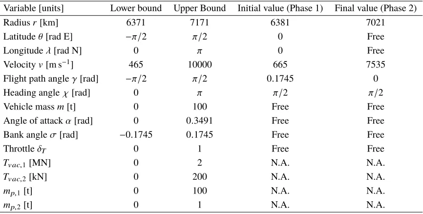
[image:21.612.77.538.82.262.2]Table 2 Lower bounds, upper bounds and boundary conditions for the Three Objective Ascent case
Variable [units] Lower bound Upper Bound Initial value (Phase 1) Final value (Phase 2)
Radiusr[km] 6371 7171 6381 7021
Latitudeθ[rad E] −π/2 π/2 0 Free
Longitudeλ[rad N] 0 π 0 Free
Velocityv[m s−1] 465 10000 665 7535
Flight path angleγ[rad] −π/2 π/2 0.1745 0
Heading angleχ[rad] 0 π π/2 π/2
Vehicle massm[t] 0 100 Free Free
Angle of attackα[rad] 0 0.3491 Free Free
Bank angleσ[rad] −0.1745 0.1745 Free Free
ThrottleδT 0 1 Free Free
Tvac,1[MN] 0 2 N.A. N.A.
Tvac,2[kN] 0 200 N.A. N.A.
mp,1[t] 0 100 N.A. N.A.
mp,2[t] 0 1 N.A. N.A.
1. Structural mass models
For the first stage, the dry mass is a function of the engine massmeng,1and propellent mass required for the first phasemp,1,
mdr y,1=−l3m˜3p,1+l2m˜ 2
p,1+l1m˜p,1+l0+meng,1 (30) ˜
mp,1=
mp,1−l4
l5 (31)
For the second stage vehicle, the dry mass was assumed to be
mdr y,2= 0.1
0.9mp,2+meng,2 (32)
The gross vehicle masses for each phase are then given by,
m0,1 =mdr y,1+mp,1+mdr y,2+mp,2 (33)
m0,2 =mdr y,2+mp,2 (34)
The vacuum thrust of the engines was used to estimate their structural mass based on an empirical linear relationship of existing commercial engines,
meng=l6Tvac+l7 (35)
publicly [46]. For the first stage engine, 0≤Tvac ≤2 MN andIs p=332 s, while for the second stage engine 0≤Tvac≤ 200 kN andIs p=352 s. Propellent masses were limited to 100 t for the first stage and 20 t for the second.
2. Objectives
The aim of the optimisation is to study the trade off between propellent efficient designs and designs that require relatively small engines. The objective functions were to minimise the gross vehicle massm0,1and the two ratios between the vacuum thrust of the stage engine, and the gross weight at the beginning of each phase. The thrust-to-weight metric also gives an indication of the vehicle loads or induced accelerations the vehicle experiences during flight. The higher the ratio between thrust and mass, the higher the loads imposed on the vehicle, thus one option is to minimise loading by minimising the thrust to weight ratio. Reducing the vacuum thrust reduces the engine performance however, which requires often longer duration trajectories and more propellant, which in turn increase the vehicle mass.
min tf,u,Tvac,1,Tvac,2,mp,1,mp,2
[J1, J2,J3]T =
m0,1, Tvac,1
g0m0,1 , Tvac,2
g0m0,2
T
(36)
3. Numerical settings
The problem was discretised using 4 DFET elements of order 7 for both states and controls, and both phases, resulting in a total of 207 optimisation variables for the outer level and 666 optimisation variables for the single level and inner level NLP. A limit of 80000 calls to the objective vector was given to the optimiser, 106 agents were deployed in the search space and the same maximum number of solutions were kept in the Archive. The initialisation of the population required between 5 seconds and 5 minutes per agent. Matching conditions between the phases were imposed on all state variables except for the mass, for which the following instantaneous drop was imposed at the stage separation:
m0,2=mf,1−mdr y,1 (37)
4. Results
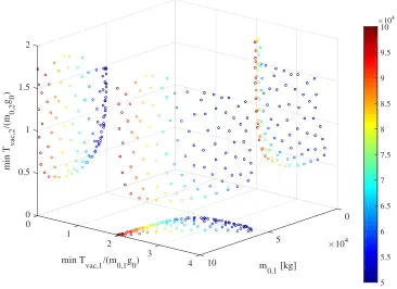
Figure 7 shows the 106 Pareto optimal solutions in the archive at the last iteration, with an additional colorbar indicating gross take-off mass. The shape of this 3D Pareto front resembles a smooth half cup. The figure shows the 3D surface in the middle, and the three orthogonal projections. As can be seen, the algorithm found a very good spread set of solutions, all of which are feasible and locally Pareto optimal up to the requested 10−6threshold.
min T
vac,1/(m0,1g0)
0 0 0 0.5 1 min T vac,2 /(m 0,2 g 0 ) 1 1.5
×104
m
0,1 [kg] 5 2 2 3 10 4 5 5.5 6 6.5 7 7.5 8 8.5 9 9.5 10 ×104
Fig. 7 Three-Objective Ascent: set of Pareto-optimal solutions, colorbar indicates gross mass of the vehicle. The 3D Pareto front is in the middle, with orthographic projections shown on each coordinate plane.
[image:24.612.120.486.72.338.2]relatively lower thrust engine of the minimum(Tvac,1/m0,1g0)case, the resulting flight path angle dips and becomes negative causing the vehicle to briefly lose altitude. The minimum second stage(Tvac,2/m0,2g0)solution is instead quite different: the first stage engine has to compensate for the relatively small second stage engine by pushing the vehicle to a higher altitude, velocity and flight path angle at the separation point. The second stage engine has to operate at maximum throttle for a comparatively longer length of time after the separation, and has a higher throttle setting during the final circularisation burn in order to compensate for its lower thrust, as shown in Fig. 9b. The total flight duration is also slightly longer than the other two.
Table 3 Design parameters for the three extreme cases of the Three-Objective Ascent case
Solution Stage Initial Propellant Dry Vacuum Thrust
∆v
mass [t] mass [t] mass [t] thrust [kN] weight ratio [km s−1] min(m0,1)
1 49.995 29.632 (59.27%) 20.363 (40.73%) 1682.611 3.432 2.836
2 8.765 7.063 (80.59%) 1.699 (19.38%) 126.100 1.467 5.664
min(Tvac,1/m0,1g0)
1 100.000 72.830 (72.83%) 27.170 (27.17%) 1930.137 1.968 4.115
2 11.789 9.717 (82.42%) 2.071 (17.57%) 200.000 1.730 6.003
min(Tvac,2/m0,2g0)
1 79.318 60.629 (76.44%) 18.689 (23.56%) 2000.000 2.571 4.565
2 4.390 3.234 (73.66%) 1.156 (26.34%) 15.124 0.351 4.606
[image:24.612.72.555.563.682.2]individually) including a breakdown of the vehicle masses with the relative percentage values with respect to the stage’s initial mass, engine vacuum thrust, thrust to weight ratio, and resulting∆vcontribution. The solution with minimum initial mass requires high ratios of vacuum thrust to initial weight, though the vacuum thrust of the engines does not reach the maximum allowed values. Propellent mass is approximately 60% of the total mass of the first stage and approximately 80% of the total of the second stage. Total∆vis of 8.5 km s−1, with the first stage contributing approximately for 2.8 km s−1 or 33% of the total, and the rest coming from the second stage. The ratio between the payload and gross vehicle mass is approximately 1%.
The solution corresponding to the minimum thrust to weight ratio of the first stage requires a larger vehicle with a substantially higher amount of propellant: its initial mass reaches the maximum allowed value for the mass of the vehicle (see Table 2), and is double the value of the previous case. Of this gross mass, approximately 70% is propellant for the first stage. The ratio between the payload mass and the initial mass is 0.5%. The total required∆vis 10.1 km s−1, with 6 km s−1coming from the second stage. The second stage engine also has the maximum possible vacuum thrust and consumes more propellant than the previous case leading to a high(Tvac,2/m0,2g0)at the cost of a minimised first stage(Tvac,1/m0,1g0).
The solution corresponding to the minimum thrust to weight ratio of the second stage requires an intermediate initial mass, approximately 60% more than the minimum initial mass case. The ratio between the payload mass and the initial mass is 0.63%, and the required∆vtotals 9.1 km s−1, evenly spread between the two stages. This is true also for the propellant mass, representing approximately 75% of the total of each stage and totalling twice as much as the minimum gross take-off mass case. The first stage engine has to compensate by taking the maximum allowed value of vacuum thrust, with the resulting thrust to weight ratio being higher than in the previous case, leading to higher induced accelerations. However, the second stage is significantly lighter than the other solutions both in terms of dry mass and propellent mass, and its engine has a vacuum thrust one order of magnitude smaller than the previous solutions.
D. Optimal Ascent and Abort Scenarios
The third test case is the multidisciplinary design of a spaceplane accounting for abort scenarios. Other studies [47] have looked at optimising the abort descent for an independently determined optimal ascent trajectory. Here, the design of the vehicle and trajectory is formulated as a multi-objective optimisation to account for the vehicle design and performance during the ascent to orbit under nominal conditions and the descent under abort conditions, for different abort scenarios.
(a) (b)
Fig. 8 Three-Objective Ascent: time-history of a) the altitude and b) the velocity for the three extreme solutions of the Pareto front in Fig. 7. The+indicates the stage separation point.
(a) (b)
Fig. 9 Three-Objective Ascent: time-history of a) the flight path angle and b) the throttle for the three extreme solutions of the Pareto front in Fig. 7. The+indicates the stage separation point.
specific timetf ail. To study the worst case, no propellent dumping was allowed.
The optimisation problem is configured to find the optimal control for the trajectories, and the optimal sizing of the wing area, which affects the downrange performance during the abort and the dry mass of the vehicle. The initial flight path angle is also set as an optimisable design parameter.
[image:26.612.77.538.77.272.2] [image:26.612.79.540.327.517.2]attempts an emergency landing. The boundary conditions for the states and controls are given in Table 4.
[image:27.612.96.518.187.377.2]Inter-phase constraints were introduced at the branching point to impose the continuity of states and controls between Phase 1 and Phase 2 and continuity of the states only between Phases 1 and 3. The throttle in Phase 3 was imposed to be zero.
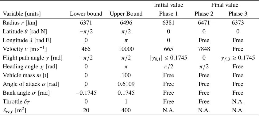
Table 4 Lower bounds, upper bounds and boundary conditions for the Optimal Ascent and Abort Scenarios case
Initial value Final value
Variable [units] Lower bound Upper Bound Phase 1 Phase 2 Phase 3
Radiusr[km] 6371 6496 6381 6471 6373
Latitudeθ[rad N] −π/2 π/2 0 0 0
Longitudeλ[rad E] 0 π 0 Free Free
Velocityv[m s−1] 465 10000 665 7848 Free
Flight path angleγ[rad] −π/2 π/2 |γ0,1| ≤0.1745 0 γf,3 ≥0.1745
Heading angleχ[rad] 0 π π/2 π/2 Free
Vehicle massm[t] 0 100 Free Free Free
Angle of attackα[rad] 0 0.6109 Free Free Free
Bank angleσ[rad] −0.1745 0.1745 Free Free Free
ThrottleδT 0 1 Free Free N.A.
Sr e f [m2] 20 400 N.A. N.A. N.A.
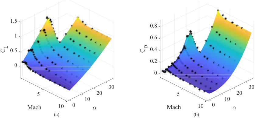
1. Aerodynamic model
Polynomial models of the lift and drag coefficients, as functions of angle of attackαand Mach numberM, were built with a non-linear least square best fit of the aerodynamic data of the X-34 vehicle [48, 49]. The polynomial models are in the form:
CL(α,M)=P2,1(α)+P2,2(α)W1(M)+P2,3(α)W2(M)
CD(α,M)=P3,1(α)+P3,2(α)W3(M)+P3,3(α)W3(M)
(38)
where Pi,j is the jth polynomial of degreei ofαwith monomial coefficients(aj,0,· · ·,aj,i+1)andWi are Weibull distributions over Mach with parameters(ςj, κj)shifted by%j, i.e.,
Wi = κi ςi
M−%i ςi
κi−1 e−
M−% i
ςi κi
(39)
the rectangular area defined byα≥20° andM ≤3, the smooth constraint
α− 35 15
8 +
M−30
27 8
−1≤0 (40)
was imposed to exclude that area. The additional path constraintM ≤0.3 was imposed on all trajectories to exclude Mach numbers for which the models extrapolated poorly. As the vehicle is not expected to fly in either of these conditions, these constraints do not affect the optimality of the results.
[image:28.612.98.517.217.412.2](a) (b)
Fig. 10 Data points, black dots, and non-linear fit surfaces of the aerodynamic coefficients: a)CLas a function
ofMandαand b)CDas a function ofMandα.
2. Wing mass model
In order to account for the change in mass due to a change of wing surface, the following mass relationship from Rohrschneider [50] was used:
mwing=©
«
Nzmland 1
1+ηSSb o d ye x p ª ®
¬
0.386
S
ex p tr oot
0.572
Kwingb0.572
str +Kctb0body.572
(41)
maximum loading of 3 multiplied by the safety factor of 1.5 for the ultimate load,η=0.15 corresponding to a control configured vehicle,Kwing=0.214 for organic composite honeycomb wing without TPS, andKct=0.0267 for integral dry carry-through of the wing beam, the lightest option available. The geometric parameters were derived from the geometry of the X-34 [48, 49]: Sex p =0.7283Sr e f,Sbody =0.6970Sr e f,bstr =1.486pSr e f,bbody =0.2785pSr e f, tr oot=0.087pSr e f, whereSr e f is a static optimisation variable.
3. Loading Constraints
As an optimisation of the gross initial mass could result in a reduction of the wing area, the following constraint on the wing loading was imposed:
m0,1 Sr e f
≤700 kg/m2
(42)
together with the limit on the dynamic pressure experienced by the vehicle in all three phases:
1 2
ρav2r el ≤60 kPa (43)
In order to limit the maximum static structural stresses, the total acceleration in all three phases was constrained to be:
Û
v2+v2γÛ2+θÛ2 ≤ (
3g0)2 (44)
The final flight path angle for the abort phase was required to be greater than−10°, and the final velocity of the abort phase had to be such thatM =0.4.
4. Objectives
The optimisation criteria are the minimisation of the spaceplane initial mass and the maximisation of the downrange in case of an abort. As the vehicle is flying along the equator, the downrange can be measured in terms of the angular difference in longitude. The problem can thus be formulated as
min tf,u,Sr e f,γ0
[J1, J2]T =
m0,1,−(λf,3−λ0,3)
T
(45)
wherem0,1indicates the mass of the vehicle at the beginning of phase 1, whileλ0,3andλf,3indicate the longitude of the vehicle at the beginning and end of phase 3 respectively.
5. Numerical settings
The first analysis performed was fortf ail=0 s. This is the worst case scenario in which the engine does not start. In this case there are only two phases as phase 1 has 0 length. The problem was discretised with 6 elements in the first phase and 3 in the second, using polynomials of order 7 for all states and controls. MACSoc was run for 20000 calls to the objective vector, 10 agents and a maximum archive size of 10. The initialisation took between 10 seconds and 40 seconds for each agent, all of which managed to find a feasible solution directly at the initialisation stage. The whole process ran for approximately 2h.
6. Results
The set of Pareto-optimal solutions is shown in Fig. 11a. The solutions are well spread and problems (17) are solved down to an accuracy of 10−6in both optimality and feasibility. The associated wing loading and downrange for all the 10 Pareto-optimal solutions are shown in Fig. 11b.
[image:30.612.79.541.317.498.2](a) (b)
Fig. 11 Abort at 0 seconds: a) Pareto front and b) wing loading vs downrange.
As the ascent and abort trajectories start concurrently, the main trade-off is on the vehicle design and aerodynamic performance. The wing loading varies inversely to the downrange, as expected. This has an effect on the flight path angle and the throttle, which in turn affect the heat flux and the total acceleration. The result is that all solutions reach the maximum possible initial flight path angle.
High downrange solutions favour larger wing areas, which translates into a higher initial mass, due to the increased drag and higher mass of the wings themselves. However, the increase in wing area, is such that the wing loading actually decreases. Thus, solutions with larger wings have a lower wing loading and are able to generate longer downrange abort trajectories.
(a) (b)
Fig. 12 Abort at 0 seconds: a) altitude vs time and b) altitude vs downrange for ascent (solid lines) and descent (dashed lines).
of the total acceleration experienced by the vehicle. All ascent phases are characterised by a maximum acceleration region in approximately the same time interval. The throttle profile, shown in Fig. 13b, differs from minimum mass solutions to maximum downrange solutions. For minimum mass solutions (small wing area) the throttle starts at maximum and remains there for a period of time, then progressively reduces down to zero, to comply with the limits on the accelerations, before finally increasing again to inject the spaceplane into orbit. Maximum downrange solutions, instead, favour a more gradual increase of the thrust and a better use of the aerodynamics.
The same analysis was then repeated for abort points at 5, 10, 15, 20, 25, 30, 35 and 40 seconds, changing the discretisation to 3 elements for each of the 3 phases. Figure 15a shows the corresponding approximations of the Pareto fronts. Interestingly, the different abort cases generate Pareto fronts which progressively converge to a single point at tf ail=30 s. Fortf ailbetween 30 s and 40 s, only one design solution exists for increasing values of the downrange. The increase of downrange is due to the increase of velocity and altitude while the size of the wings remain unchanged to keep the initial mass to the minimum. Thus, if the vehicle operates properly for at least 30 seconds, it gains so much velocity and altitude that, in the case of an abort, the downrange does not benefit from large wings. The same conclusion can be drawn from Fig. 15b that shows the wing loading of all solutions for all abort points.
(a) (b)
Fig. 13 Abort at 0 seconds: time histories for a) total acceleration and b) engine throttling for ascent (solid lines) and descent (dashed lines).
V. Conclusions
This paper presented a novel approach to the solution of multi-phase, multi-objective optimal control problems applied to the ascent, re-entry and abort scenarios for different hypothetical vehicles. The approach, combining Direct Finite Elements in Time transcription with Multi-Agent Collaborative Search, provided a robust and accurate method to compute sets of Pareto optimal solutions. In particular the smooth transition from Chebyshev to Pascoletti-Serafini scalarisation allows for a balanced and effective local refinement of the solutions and a global exploration of the search space.
The approach was first validated on a known case from the literature confirming the ability to accurately identify the optimal values for each individual objective function and to reconstruct a well spread set of locally Pareto optimal solutions. The application to the three objective case demonstrated the ability of the algorithm to generate a well spread Pareto front even in the case of more than two objectives. Furthermore, the solutions in the Pareto set give a unique insight on the impact of system design choices and an optimal trade-off between system sizing and control law, allowing the decision maker to make entirely different strategic choices depending on what is considered more important.
The abort scenario case provided an unexpected result that could not be derived from a single objective optimal control formulation of the problem: the trade-off on the wing loading affects the ascent trajectory as the aerodynamics of the vehicle changes due to the need to improve flight performance during descent, however this is true up to a limit abort time of about 30 s. Beyond that point there is no trade-off and only one optimal configuration exists because a high wing surface solution is also heavier, and the increase in gliding capabilities does not compensate for the increase of mass and thus the lower starting velocity and altitude of the abort phase.
(a) (b)
Fig. 14 Abort at 0 seconds: time histories of a) flight path angle and b) heat flux for ascent (solid lines) and descent (dashed lines).
solution of multi-objective optimal control problems is devised any direct transcription method is applicable and can be paired to the MACSoc solver. Future implementations will consider these additional pairings with other transcription methods.
Appendix
[image:33.612.75.535.458.635.2]Table 5 reports the coefficients used for the aerodynamic model for the Optimal Ascent and Abort Scenarios case.
Table 5 Coefficients for the aerodynamic model
Coeff. Value Coeff. Value Coeff. Value
a1,0 -6.378335936032101e-02 ς1 1.344774373794846e+00 a5,3 -1.683702441539749e-04 a1,1 1.976923220591986e-02 ς2 1.542614382500486e+00 a6,0 8.869412111210242e+00 a1,2 2.973963976446931e-04 %1 -3.100574615791786e+01 a6,1 7.482402265848023e-01 a2,0 -3.349264465313049e+05 %2 -9.123166455265215e-02 a6,2 2.604898066115986e-02 a2,1 6.001178833841350e+05 a4,0 4.941304084167961e-02 a6,3 2.689898581212407e-04 a2,2 -2.862064269172794e+04 a4,1 -2.771101541363621e-03 κ3 1.348770573128532e+00 a3,0 4.398289382706495e-01 a4,2 4.195518696508440e-04 κ4 1.376496163657956e+00 a3,1 6.555024080116524e-02 a4,3 6.144719928912810e-06 ς3 1.004292397340135e+00 a3,2 -4.816546419307238e-04 a5,0 -8.408713897701869e+00 ς4 1.053245533842992e+00 κ1 1.088199979257513e+00 a5,1 -6.942588805953275e-01 %3 -2.715562764314760e-01 κ2 1.523372394108941e+00 a5,2 -2.602381527566895e-02 %4 -3.464086848960685e-01
Acknowledgments
(a) (b)
Fig. 15 Comparison of Pareto optimal solutions for different abort times: a) downrange versus initial mass, b) wing loading for each solution ID.
References
[1] Stryk, O. V., “Numerical Solution of Optimal Control Problems by Direct Collocation,”Optimal Control Calculus of Variation,
Optimal Control Theory and Numerical Methods, Birkhauser Verlag, 1993.
[2] Herman, A. L., and Conway, B. A., “Direct optimization using collocation based on high-order Gauss-Lobatto quadrature rules,”Journal of Guidance, Control, and Dynamics, Vol. 19, No. 3, 1996, pp. 592–599. doi:10.2514/3.21662.
[3] Vasile, M., “Robust Optimization of Trajectory Intercepting Dangerous NEO,”Proceedings of the AAS/AIAA Aerodynamics
Specialist Conference, Monterey, California, Aug 2002.
[4] Vasile, M., and Bernelli-Zazzera, F., “Optimizing Low-Thrust and Gravity Assist Maneuvres to Design Interplanetary Trajectories,”The Journal of the Astronautical Sciences, Vol. 51, No. 1, 2003. January-March 2003.
[5] Betts, J. T.,Practical methods for optimal control and estimation using nonlinear programming, Advances in Design and Control, SIAM, 2010.
[6] Vasile, M., “Finite Elements in Time: A Direct Transcription Method for Optimal Control Problems,”AIAA/AAS Astrodynamics
Specialist Conference, Guidance, Navigation, and Control and Co-located Conferences, Toronto, Canada, 2-5 Aug 2010. doi:0.2514/6.2010-8275.
[7] Garg, D. A., Patterson, M., Hagger, W., Rao, A. V., Benson, D. A., and Huntington, G. T., “A Unified Framework for the Numerical Solution of Optimal Control Problem Using Pseudospectral Methods,”Automatica, 2010.
[9] Zhu, Q. J., “Hamiltonian Necessary Conditions for a Multiobjective Optimal Control Problem with Endpoint Constraints,”
SIAM Journal on Control and Optimization, Vol. 39, No. 1, 2000, p. 97–112. doi:10.1137/S0363012999350821.
[10] de Oliveira, V., Silva, G., and Rojas-Medar, M., “A class of multiobjective control problems,”Optimal Control Applications
and Methods, Vol. 30, 2009, pp. 77–86. doi:10.1002/oca.863.
[11] Kien, B., and N.C. Wong, J. Y., “Necessary conditions for multiobjective optimal control problems with free end-time,”SIAM
Journal on Control and Optimization, Vol. 47, No. 5, 2010, pp. 2251–2274. doi:10.1137/080714683.
[12] Oliveira, V. A., and Silva, G. N., “On Sufficient Optimality Conditions for Multiobjective Control Problems,”Journal of Global
Optimization, Vol. 64, No. 4, 2016, pp. 721–744. doi:10.1007/s10898-015-0351-y.
[13] Ngo, T.-N., and Hayek, N., “Necessary conditions of Pareto optimality for multiobjective optimal control problems under constraints,”Optimization, Vol. 66, No. 2, 2017, pp. 149–177. doi:10.1080/02331934.2016.1261349.
[14] Ober-Blöbaum, S., Ringkamp, M., and zum Felde, G., “Solving multiobjective optimal control problems in space mission design using discrete mechanics and reference point techniques,”51st IEEE Annual Conference on Decision and Control, Maui, Hawaii, 10-13 Dec 2012, pp. 5711–5716. doi:10.1109/CDC.2012.6426285.
[15] Kaya, C. Y., and Maurer, H., “A numerical method for nonconvex multi-objective optimal control problems,”Computational
Optimization and Applications, Vol. 57, No. 3, 2014, pp. 685–702. doi:10.1007/s10589-013-9603-2.
[16] Pascoletti, A., and Serafini, P., “Scalarizing vector optimization problems,”Journal of Optimization Theory and Applications, Vol. 42, No. 4, 1984, pp. 499–524. doi:10.1007/BF00934564.
[17] Pagano, A., and Mooij, E., “Global launcher trajectory optimization for lunar base settlement,”AIAA/AAS Astrodynamics
Specialist Conference, Guidance, Navigation, and Control and Co-located Conferences, Toronto, Canada, 2-5 Aug 2010. doi:10.2514/6.2010-8387.
[18] Bairstow, B., de Weck, O., and Sobieszczanski-Sobieski, J., “Multiobjective Optimization of Two-Stage Rockets for Earth-To-Orbit Launch,”47th AIAA/ASME/ASCE/AHS/ASC Structures, Structural Dynamics, and Materials Conference, 2006, p.
1720.
[19] Roshanian, J., Bataleblu, A. A., and Ebrahimi, M., “Robust ascent trajectory design and optimization of a typical launch vehicle,”Proceedings of the Institution of Mechanical Engineers, Part C: Journal of Mechanical Engineering Science, 2018. doi:10.1177/0954406217753460.
[20] Coverstone-Carroll, V., Hartmann, J. W., and Mason, W. J., “Optimal multi-objective low-thrust spacecraft trajectories,”Computer
methods in applied mechanics and engineering, Vol. 186, No. 2, 2000, pp. 387–402. doi:10.1016/S0045-7825(99)00393-X. [21] Englander, J. A., Vavrina, M. A., and Ghosh, A. R., “Multi-Objective Hybrid Optimal Control for Multiple-Flyby Low-Thrust
![Fig. 2Optimal descent trajectory: Pareto optimal solutions stored in the archive A at the end of the optimisa-tion process and the two published single objective solutions from Betts [5].](https://thumb-us.123doks.com/thumbv2/123dok_us/1351065.88737/19.612.79.540.299.478/optimal-trajectory-solutions-optimisa-process-published-objective-solutions.webp)