A Furcated Visual Collision Avoidance System for an Autonomous Micro Robot

City, University of London Institutional Repository

Citation

:

Isakhani, H., Aouf, N. ORCID: 0000-0001-9291-4077, Kechagias-Stamatis, O.

and Whidborne, J. F. (2018). A Furcated Visual Collision Avoidance System for an

Autonomous Micro Robot. IEEE Transactions on Cognitive and Developmental Systems,

doi: 10.1109/TCDS.2018.2858742

This is the accepted version of the paper.

This version of the publication may differ from the final published

version.

Permanent repository link:

http://openaccess.city.ac.uk/id/eprint/23186/

Link to published version

:

http://dx.doi.org/10.1109/TCDS.2018.2858742

Copyright and reuse:

City Research Online aims to make research

outputs of City, University of London available to a wider audience.

Copyright and Moral Rights remain with the author(s) and/or copyright

holders. URLs from City Research Online may be freely distributed and

linked to.

A Furcated Visual Collision Avoidance System for

an Autonomous Micro Robot

Hamid Isakhani,

Member, IEEE

, Nabil Aouf, Odysseas Kechagias-Stamatis, and James F. Whidborne,

Senior

Member, IEEE

Abstract—This paper proposes a secondary reactive collision avoidance system for micro class of robots based on a novel approach known as the Furcated Luminance-Difference Process-ing (FLDP) inspired by the Lobula Giant Movement Detector, a wide-field visual neuron located in the lobula layer of a locust

nervous system. This paper addresses some of the major collision avoidance challenges; obstacle proximity & direction estimation, and operation in GPS-denied environment with irregular lighting. Additionally, it has proven effective in detecting edges indepen-dent of background color, size, and contour. The FLDP executes a series of image enhancement and edge detection algorithms to estimate collision threat-level which further determines whether or not the robot’s field of view must be dissected where each section’s response is compared against the others to generate a simple collision-free maneuver. Ultimately, the computation load and the performance of the model is assessed against an eclectic set of off-line as well as real-time real-world collision scenarios validating the proposed model’s asserted capability to avoid obstacles at more than 670 mm prior to collision, moving at 1.2 ms-1with a successful avoidance rate of 90% processing at 120 Hz on a simple single core microcontroller, sufficient to conclude the system’s feasibility for real-time real-world applications that possess fail-safe collision avoidance system.

Index Terms—Autonomous robots biologically-inspired colli-sion avoidance furcated luminance-difference processing (FLDP) direction and proximity estimation.

I. INTRODUCTION

C

OLLISION avoidance is an intricate and vital block within an autonomous system for which, various hard-ware and softhard-ware solutions are being tested and studied in order to develop a reliable and robust system capable of generating collision-free control commands independent of human supervision and control. Limited payload delivery of the smaller robots hinders the development of their au-tonomous control systems, though certain algorithms imple-mented on micro-sized processors deliver a reasonably effi-cient collision-free maneuvering capability [1]–[5]. However, substantial hardware advances are emerging in development of larger aerial robots (<20kg) bolstered by their greater payload capacity accommodating sophisticated sensors and computers to perform fully autonomous take-off and landing [6]–[8],

H. Isakhani is with the Computational Intelligence Laboratory, School of Computer Science, University of Lincoln, Lincoln LN6 7TS, UK. (e-mail: [email protected])

N. Aouf and O. Kechagias-Stamatis are with the Signals and Auton-omy group, Centre for Electronic Warfare, Information and Cyber, Cran-field University, Defence Academy, Swindon SN6 8LA, UK. (e-mail: [email protected], [email protected])

J.F. Whidborne is with the Centre for Aeronautics, School of Aerospace, Transport and Manufacturing, Cranfield University, Bedford MK43 0AL, UK. (e-mail:[email protected])

stabilization and localization [9]–[11], collision avoidance [12], [13], and aerobatic flight [14], [15]. Hence, the software developments for micro class of mobile robots must be further explored to compensate for hardware deficiencies.

Contemporary hardware solutions for collision sensing and avoidance, for instance, a planar laser range finder (LIDAR) is much heavier than the available payload on a small category unmanned aircraft. On the other hand, active range finders such as the Microsoft Kinect 2 are incapable of operating outdoors, hence one of the most feasible solutions remaining, could be the fusion of a lightweight camera and a robust computer vision algorithm. Salient features of vision-based solutions specifically for aerial robotic applications include its simplic-ity, reduced weight, and cost, justifying researchers’ focus on this technique. Ground robot application of a vision-based machine learning algorithm to avoid obstacles autonomously at a processing frequency of 7 Hz and a forward velocity of 5 ms-1in a complex cluttered environment produced satisfactory results (<2% errors) [16] which was improved further in aerial applications of on-board depth computation and learning range classifiers in real-time, facilitating autonomous collision-free flight over 100 m [17]. Although, these monocular vision-based solutions satisfy the hardware limitations, they fail to cope with the curbed processing power as they are computa-tionally expensive, thus a simple biologically inspired vision-based model is proposed, whose principle of operation is vision-based on difference frame processing, a rather appealing behavior observed in the lobula layer of the locust visual neuron that performs an extremely simple process of image segmentation by computing absolute gray scale image difference over two consecutive frames [18]–[22].

requirement of this research that is an extreme limitation on computational power. Therefore, a successfully tested, simple, and comprehensive computational model of a Lobula Giant Movement Detector (LGMD) is considered here to provide a source of inspiration for this study.

An LGMD responds decisively to an approaching object on collision course, facilitating collision-free flights in vast and dense swarms [26]. It is a bilaterally paired motion sensitive neuron that responds robustly to images of objects approaching on a collision course by integrating input signals from the photoreceptors. The computational model of an LGMD was pioneered by Rind et al. [27], and has continuously evolved over the years, with the current version being implemented in ground robot navigations and autonomous cars involving diverse set of adaptations and modifications with respect to their applied field. One of the outstanding features of LGMD is the neuron’s capability to detect direction of an obstacle’s motion involving approach, translation, and recession [28], [29], which is achieved by the integration of a feed-forward in-hibition, and ON/OFF channels. However, greater robustness, precision, and computational simplicity could be achieved by enhancing these connectomes with complementary modules that emulate the near-exact intricate behavior of an effective insect-vision suitable for mobile robotic applications.

Continuous attempts are being made to contribute towards modification of an LGMD model, including the pioneers of the original model, Sztarker and Rind [30] whose work found that, apart from the conventional LGMD and DCMD (Descending Contra-lateral Movement Detector), there are additional neu-rons in thelocustoptic lobe that respond to expanding stimuli and have been implicated in triggering evasive responses, naming the additional neural network as LGMD2. Furthermore they provide evidence to prove that the two share many key features including direction selectivity, but neither its role in overall behavior nor its post-synaptic target neurons have been studied in detail yet, offering a potential subject of research for neuroscientists.

Silva et al. [31], [32] proposed a modified LGMD archi-tecture integrating two previous LGMD models to implement features such as noise immunity proposed in [18], [33] and direction detection proposed in [19], the optimized model is validated against a set of test cases (collision scenarios), where a successful filtering of isolated excitations is performed to prevent the perturbations from contributing to the excitation of the LGMD cell. Silva goes on to demonstrate that the neural architecture introduced in [18] was unsatisfactory when tested for shrinking stimuli whereas the model in [19] detected obstacle motion direction in depth. However, the latter is not immune to signal noise, which could cause faulty collision alarms in case of a perturbed input signal. Hence, fusing the advantages of the two models, a modified model is achieved that can distinguish an approaching from a receding object while ignoring input signal noise.

[image:3.612.316.559.72.132.2]

Cuadri et al. [26], among others, introduced two comple-mentary modules called the Attention Focusing Mechanism and Topological Feature Estimator to augment their model’s versatility and efficiency, where the first module aims to optimize the use of computational power by limiting the

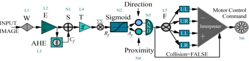
Fig. 1. Schematic illustration of Furcated Luminance-Difference Processing (FLDP) model. The proposed architecture consists of 5 layers (L1,L2,...,L5) of processing namely, linear time-invariant filter (W), excitation (E), adaptive histogram equalization (AHE), threshold (T), and furcation (F). Followed by 6 single processing nodes (N1,N2,...,N6) namely, the direction detector, depth estimator, summation, sigmoid transformer, AND logic gate, and motor control command generator node.

processing core to focus only on the frame zones that exhibit maximum activity, and the second module aims to extract further information about the current alarming status, par-ticularly making a quick categorization of the approaching obstacle. Similar to the afore mentioned findings, in this paper, a biologically-inspired computational model is designed and tested to perform an effective collision avoidance onboard a mobile robot based on a novel approach called the Furcated Luminance-Difference Processing (FLDP). This solution ad-dresses some of the major collision avoidance challenges using complementary modules such as Image Stabilizer, Contrast Rectifier, and Proximity Estimator, to reduce motion-induced vibrations, rectify irregular lighting, and distinguish between a large faraway object and a small imminent one, respec-tively. Experiments, results and performance assessments are presented systematically to bolster the asserted capabilities. Although the pure engineering contributions of this research might not be comparable to the current literature, we mainly aim to appreciate and inspire study on the biological solutions to address engineering problems.

The organization of this paper is as follows, Section II intro-duces the structure of the proposed model and its processing layers. Section III demonstrates the off-line experiments and testing of the algorithm. Section IV illustrates real-world test setup and results. Section V assesses the results and compares the performance of the model with the current literature. And ultimately, section VI offers concluding remarks.

II. MODELDESIGN

The reactive collision avoidance model proposed here is based on the luminance difference processing exhibited by an LGMD that is sensitive to looming objects causing changes in luminance projected on the photoreceptor cells of locust

adaptive histogram equalization layer (AHE), threshold layer (T), and furcation layer (F), preceded by six single processing nodes (N1,N2,...,N6) namely, the direction detector, depth estimator, summation, sigmoid transformer, AND logic gate, and motor control command generator node.

As shown in Figure 2(a), the input imagesaf,af−1and so

on, are a sequence off number of 2D arrays with a dimension

kxlpixels, where each pixel value(u, v)∈[0−255]distributed panoramically along u(horizontal axis) and v(vertical axis) representing gray scale image frames of the input signal illustrated in Figure 1.

A. Layer-W

Since aerial robots exhibit vibrations over various frequen-cies, a linear time-invariant filter such as a Wiener filter [35] is introduced as the first layer to eliminate noise (undesirable blur) adaptively within the input image exerting a minute computation load (∼4 milliseconds to process 1 frame) by estimating the local mean (µf) and variance (σf) around each

pixel as,

µf = 1

N M N

X

u=1 M

X

v=1

af(u, v) (1) and

σ_f2= 1

N M N

X

u=1 M

X

v=1

a2_f(u, v)−µ2_f, (2) where N and M are the local neighborhood of each pixel along horizontal and vertical axis respectively in the input image, which further creates a pixel-wise filter using,

bf(u, v) =µf+σ 2 f−w

2 σ2

f

[af(u, v)−µf] (3) wherebf is the filtered input signal and w2 _{is the noise}

vari-ance (additive noise) which is not specified for our application, hence considered as the average of all the locally estimated variances.

B. Layer-E

The filtered signal is then fed to the excitation layer that estimates the luminance difference of two consecutive input image frames by computing the absolute difference of the value of each pixel within the 2D array of an image with respect to its previous time-step, mathematically,

Ef(u, v) =|bf(u, v)−bf−1(u, v)| (4)

whereEf is the output of the excitation layer at frame-f,bf

and bf−1 are the filtered luminance at current and previous

framesf andf −1, respectively.

C. Layer-AHE

The next processing layer is the adaptive histogram equal-izer (AHE) [36] that enhances the excitation frame’s contrast, facilitating operation in an environment with an irregular lighting by defining a fine boundary separation along obstacle edges through subdivision and interpolation scheme. As shown

[image:4.612.329.540.73.155.2]

(a) (b)

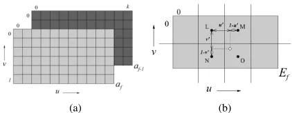
Fig. 2. Input data representation. (a) Schematic illustration of a sample input data that consists of a sequence of image frames denoted byf, each containing

kxlpixels (kandl∈[0-255]) distributed panoramically over (u,v) plane. (b) Schematic illustration of contextual regions (2x2 array) of a sample point in an image frame with centers denoted as L, M, N, and O where local gray-level mappings (gL(i),gM(i),gN(i), andgO(i)) are based on the histogram of the

contained pixels in the input frame, i being the original pixel intensity for the sample point. The gray-level attribute (denoted by a white dot) is determined by the gray-value distribution in its neighboring contextual regions.

in Figure 2(b), gray-level attribute (denoted by a white dot) is determined by the gray-value distribution in its neighboring contextual regions (2x2 array) of a sample point in an image frame with centers denoted as L, M, N, and O where local gray-level mappings (gL(c), gM(c), gN(c), and gO(c)) are based on the histogram of the contained pixels in the input frame. Considering c as the original pixel intensity for the sample point, we compute its new value by bilinear interpola-tion of the gray-level mappings that were calculated for each of the neighboring contextual zones as,

c0(u0, v0) ={(1−v0)((1−u0)gL(c) +u0gM(c))

+v0((1−u0)gN(c) +u0gO(c))} (5)

Hereu0andv0are the normalized distances with respect to the point L. The optimal contrast is thus calculated by dividing the entire image frame into such rectangular contextual elements shown in Figure 2(b) (a sample zone), and then tile-mapped to attain a whole contrast-equalized image as,

Cf(u, v) =



   

c0₁₁ c0₁₂ · · · c0_1k c0₂₁ c0₂₂ · · · c2k

..

. ... . .. ...

c0_l1 c0_l2 · · · c0_lk



   

(6)

whereCf is the concatenation of all the contextual regions alonguandv forming a 2D array of pixels with the original dimension of the input image,kxl.

D. Layer-S

The obtained contrast-corrected image Cf is added to the excitation image Ef to get,

Sf =ρs× |Ef+Cf| (7)

The summed output is treated with a sensitivity factor, ρs ∈

E. Layer-T

Furthermore, the resulting summed data Sf is passed

through a simple binary thresholding image segmentation process,

Tf(u, v) =

(

1 (White) , if Sf(u, v)≥Tr

0 (Black), if Sf(u, v)< Tr

(8) Here the output Tf converts the input matrix Sf into binary

dataset and replaces all pixels with luminance greater than the defined threshold (Tr) with the value 1 (white) and replaces

all other pixels with the value 0 (black). Tr, a global image

threshold is a scalar value determined using Otsu’s method [37]. It is a function of zeroth- and the first-order cumulative moments of the gray-level histogram of the input image.

F. Response Generation Node

Ultimately, at this node the excited (white) pixels that have passed the threshold (Tr) are summed along both dimensions of the array to generate a system response as,

Rf(u, v) = k

X

u=1 l

X

v=1

|Tf(u, v)| (9)

which is then fed to the spike generator to interpret the model response (collision alarms) as spikes. This is accomplished by transforming the response signal into a sigmoid function as,

Af = (1 +e−Rf/scell₎−1 ₍₁₀₎

wherescellis the total number of the excited pixels that have passed the threshold, and since Rf is greater than zero, the

normalized spiking response,Af ∈[0.5−1.0].

G. Direction and Depth Estimation Nodes

The generated spiking response is then interpreted to esti-mate the collision threat-level and nature of the threat, that is its course and proximity. First the direction of obstacle’s motion relative to the robot is determined by comparing average spiking response over four time-steps using a small amount of memory that records consecutive spike values (accurate to the thousandths place) to check for any persistent increase or decrease implying obstacle approach or recession, respectively. This is achieved by assigning the direction of an obstacle’s motion relative to the robot with a binary value ∈

[0,1] using the condition,

Direction=



 

 

Approaching= 1, if avgAf >avgAf−1

Receding= 0, if avgAf <avgAf−1

Stagnant= 0, otherwise

(11) and then estimating the obstacle’s proximity relative to the robot using the condition,

Depth=

(

Near= 1, if avgAf >(δ×avgAf−1)

Far= 0, otherwise (12) where avgAf is an average value of Af over 4 time-steps, and δ = 1.35, is an empirically estimated coefficient that

Fig. 3. Schematic illustration of furcation process, where the input image frames are dissected to form individual image frames (four in this case) each representing one section of the robot’s field of view namely, upper-left (UL), upper-right (UR), lower-left (LL), and lower-right (LR).

determines the nature of generated spikes implying if a threat is distant or imminent which in turn facilitates a prudent avoidance-decision making. The logic bolstering this function is

H. Furcation Node

Direction and depth estimation nodes lay the foundation of the furcation process which performs a simple dissection of the input image frame into any number of symmetric quarters depending on the application. However, to further simplify the computation, an AND logic gate is introduced to decide whether or not to initiate the process of furcation by boolean multiplication expressed as,

Furcate= Direction AND Depth (13) Following the AND gate truth table, the furcation process is not initiated if either of the parameters ‘direction’ or ‘depth’ is OFF, whereas if both parameters are turned ON exhibiting state 1, the algorithm furcates the output of thresholding layer to form individual image frames each representing one section of the observer’s field of view, illustrated in Figure 3. This node is of great significance to this research as it provides a simple yet effective solution for the challenging task of collision-free trajectory planning. It must be noted that the robot’s degree of freedom (DOF) decides the number of sections FOV is split during the furcation process. Further processing is similar to the previous section but performed on four quarter images in parallel. Furcation of Tf array is

represented as,

Tf₁(x1, y1) =Tf(

−u

2 ,

v

2) (14)

Tf2(x2, y2) =Tf(

u

2,

v

2) (15)

SimilarlyTf₃ andTf₄ are computed to be fed simultaneously to the spike generator as,

Rf1(x1, y1) =

k1 X

x1=1

l1 X

y1=1

|Tf1(x1, y1)| (16)

and

Af₁= (1 +e−Rf1/mcell₎−1 ₍₁₇₎

where mcell is the total number of the excited pixels that have passed the threshold, and sinceRf₁ is greater than zero, the normalized spikes, Af1 ∈ [0.5−1.0], where 1.0 (spike)

[image:5.612.348.528.58.149.2]

(a)

[image:6.612.316.556.52.228.2]

(b)

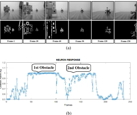
Fig. 4. Typical spiking response for an approaching obstacle. (a) Processed image frames (lower row) and raw input image frames (upper row) extracted from the input collision movie where the robot is moving at a linear velocity of 1.2 ms-1 _{towards two static obstacles of 0.5 m and 1 m wide on the left}

and right side of its field of view, respectively. (b) Spiking response for the illustrated collision movie, where the spikes exceed 0.95 border from 40th_and

135th_{frame for the first and second obstacle, respectively, implying that the}

obstacles are detected more than 3 seconds prior to contact.

I. Motor Command Generation

Further the average response over four time-steps (4 frames) is computed as,

avgAf₁ =

P4

j=0A(f−j)1

4 (18)

Similarly, the average response of the remaining quadrants (Af₂, Af₃, Af₄) are computed in parallel which are further compared against each other to estimate the most secure path (quadrant with the least average excitation) as,

MotorCmd=avgAf1−avgAf2−avgAf3−avgAf4 (19)

where the minus sign (−) represents ‘comparing’ of quad-rants, and ‘MotorCmd’ represents the quadrant with the least collision-threat level for which a Pulse-Width Modulation (PWM) signal is generated to control the turning radii (servo position) of the robot depending on the collision-threat level to navigate the robot through the estimated secure quadrant. Detailed experimental results and analysis of the proposed algorithm for different scenarios, velocities, and test environ-ments are described in further sections.

III. OFF-LINETESTING OFCOLLISIONAVOIDANCE

MODEL

A comprehensive off-line analysis of the proposed collision avoidance model is conducted and briefly demonstrated along with the inferences drawn for a wide range of collision scenarios. The collision scenarios emulated in this section assess specific modules introduced as the proposed model’s novelties including; static obstacle detection, obstacle direction detection, obstacle proximity estimation, and operation in complex backgrounds. In order to conduct a prudent off-line

(a)

[image:6.612.55.294.54.255.2]

(b)

Fig. 5. Model response to evaluate edge detection capability. (a) represents 1st_{, 30}th _{and 60}th_{image frames extracted from the column detection movie}

(90fps), respectively. This scenario involves an obstacle (column) spanning ground to ceiling built with the same granite used in the background wall, approach the robot at a linear velocity of 1.4 ms-1_{traveling a distance of 5.6 m}

in 4 seconds towards the right half of robot’s field of view. (b) demonstrates the output spiking response of the model for the left and right half of the robot’s field of view where the detected obstacle (column) causes elevated spike levels indicated in right neuron.

analysis, a complete set of input data are gathered to test the model for various possible scenarios preparing the algorithm for a successful real-time real-world application. Input dataset collection is performed systematically considering every vital parameter such as field of view (FOV=90◦), data acquisition frequency (30Hz), image resolution, dimension, and format (320x240 Pixels in gray-scale). Similarly, the collision scenar-ios are orchestrated precisely by defining sample trajectories, various constraints, obstacles, and backgrounds to emulate real-world conditions.

Further, the model in its simplest form is fed with the collected input data to analyze the role of each processing node individually and calibrate them consistently. Once the model produces the desired response, modulation and enhancement of the algorithm is performed by introducing complementary modules to fulfill the task specific objectives described previ-ously.

A. Collision Avoidance System

The input data presented here are a sample representation of the collision scenarios orchestrated to test individual features of the proposed model. This sample involves an observer (robot) moving at a linear velocity of 1.2 ms-1 towards two static obstacles of 0.5 m and 1 m wide on the left and right side of the robot’s field of view (90◦), respectively. These obstacles are placed clearly on the collision course and must eventually be avoided. Figure 4 illustrate sample image frames extracted from the input collision movie.

(a)

[image:7.612.55.293.54.266.2]

(b)

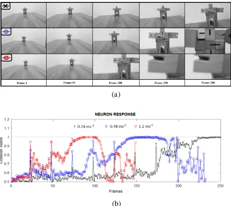
Fig. 6. Model response to evaluate model consistency. (a) Represents 1st

to 200th_{image frames at 50 frame intervals extracted from the}

consistency-evaluation movies (recorded at 90fps for three linear velocities 0.24, 0.48, and 1.2 ms-1 _{ordered from top to bottom respectively). This scenario involves a}

brightly colored static obstacle with a 1.2 m separation looming in order to trigger collision avoidance. (b) Demonstrates the output spiking response of the model over 250 frames where the black cross, blue circles, and red squares correspond to three linear velocities 0.24, 0.48, and 1.2 ms-1_{, respectively.}

When the collision alarm elevation reaches 1.0, it indicates a definite potential threat.

The model responds to the looming obstacle by increasing the collision alarm (spikes) shown in Figure 5, as the column nears, gradually the right half of the robot’s field of view is activated, elevating the spike levels in the right neuron response colored in red crosses. Further, the spike interpreter generates left-steering motor control commands that maneuver the robot away from the pillar. It is evident that the model successfully detects like-colored obstacles and differentiates edges independent of their size, color and contour.

2) Model Consistency: A rather simple scenario was de-signed to evaluate the proposed model’s response agility for various forward linear velocities. Here the robot approaches a brightly colored static obstacle with an initial separation of 1.2 m at 0.24, 0.48, and 1.2 ms-1corresponding to black cross, blue circle and red square, shown from top to bottom in Figure 6(a), respectively. The spiking response for all three cases are presented in Figure 6(b), which illustrates the black cross, blue circles, and red squares spike level rise to 1.0 from the 200th, 130th_{, and 70}th _{frame. Using the equation 20, we compute}

distances prior to a potential collision as 660, 510, and 300 mm, for the velocities in ascending order, respectively.

IV. REAL-TIMEREAL-WORLDEXPERIMENTATION

In order to validate the proposed algorithm, we demonstrate a real-time implementation of the model on a ground robot tested against a number of real-world collision scenarios involving multiple obstacles of varying color, background, dimension, and contour.

The proposed model is implemented on a 3-DOF (degree of freedom) ground robot designed and fabricated at the

Un-(a) (b)

Fig. 7. Robotic platform. (a) Assembled platform used for real-time real-world experimentation. (b) Simplified circuit connection depicting every component involving a basic 2-Megapixel CMOS sensor, an Atmel ATmega328 8-bit AVR micro-controller, basic servos and motors, and a ground control station PC (Intel Core i5-6500, 8GB RAM).

manned Autonomous Systems Laboratory (UASL), Cranfield University. It exhibits the necessary agility to accomplish successful collision avoidance using a DC motor, 9g servo motor, Arduino nano development board, motor shield, and a 2-Megapixel CMOS sensor. The Atmel ATmega328 8-bit AVR micro-controller with a maximum of 20 MHz operating frequency built into an Arduino development board is imple-mented to interface the robot with the proposed algorithm developed in MATLAB. Image frames captured by the CMOS sensor are transmitted through a USB cable to the ground control station (Intel Core i5-6500, 8GB RAM) where the images are processed and motor control commands generated. These commands are transmitted through the micro-controller to the servo and motor shield to control the robot’s locomotion. The conventional robotic differential steering was substi-tuted with an Ackerman steering to replicate near-exact real-world four wheel vehicle dynamics posing greater maneuver-ing challenges as a result of underactuation. The schematic illustration of the designed robot, test platform and circuit connections are shown in Figure 7.

A. Real-World Collision Scenario

As mentioned in Section II-H, the robot’s field of view is bifurcated here (3-DOF Robot). Initially the algorithm is executed in MATLAB and the robot launched along the trajectory. The robot is assigned to travel along a specified path through two waypoints 2 m apart steered with the help of the FLDP’s servo commands interfaced through an Arduino micro-controller. The path of the robot is impeded with two obstacles, 0.15 m and 0.2 m high, laid 0.7 m apart. The robot moves with a linear forward velocity of 1.5 ms-1_{traversing the}

[image:7.612.316.559.63.166.2]

(a)

(b)

[image:8.612.55.295.63.328.2]

(c)

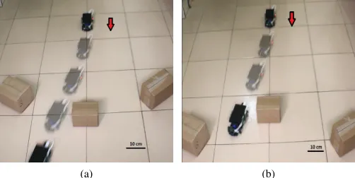
Fig. 8. Real world experimentation. (a) Blended frames of the top-view movie captured while robot travels the trajectory, involving a drift from left to right (indicated by the red arrow) through two obstacles of height, 0.15 m and 0.2 m laid 0.7 m apart, respectively. The linear velocity of the robot is 1.5 ms-1 _{traveling a total distance of 2 m without collision. (b) Robot’s field}

of view where random obstacles are detected and avoided as a result of furcated luminance-difference processing. (c) Presents the spiking response of the algorithm with respect to potential collision threats where the spikes for obstacles 1 and 2 are annotated at frames-20 and 40, respectively. This implies that the system initiates avoidance at approximately 670 mm prior to collision.

of a right steering command shown in Figure 8(b), the entire process of consecutive obstacle avoidance is completed in 20 frames (0.6 seconds), initiated at frame-20 and completed by frame-40. Substituting the equation 20 with, initial obstacle-robot separation (I=1m), frame number at which the avoid-ance is initiated (x=20th_{)(Figure 8(c)), velocity of the robot}

(v =1.5ms-1_{), processing frequency (f =90Hz), we obtain}

the proposed model’s capability to avoid arbitrary real-world obstacles at 670 millimeters prior to collision.

B. Arbitrary Standard Collision Scenarios

In order to realize the ultimate objective of our proposed algorithm, an arbitrary set of conventional collision cases encountered by a generic robot was orchestrated. Figure 9(a-d) illustrates four individual scenarios tested for at least five trials generating more than ∼80% successful collision-free maneuvering of the robot through obstacles laid in various formations. For these tests, the robot was assigned to traverse a straight trajectory connecting two waypoints from extreme left to extreme right hand side. The velocity of the robot remained linear at ∼1 ms-1 _{traveling an approximately 1.5}

m distance crammed with 0.1 m high obstacles (∼40 g crisp packets) whose flexible profile proved that the algorithm remains independent of obstacle contour, dimension, and color.

(a) (b)

[image:8.612.308.565.66.282.2]

(c) (d)

Fig. 9. Standard collision scenarios, involve a ground robot drifting at a linear velocity of∼1 ms-1 _{traveling an approximately 1.5 m long trajectory}

connecting two waypoints from left to right saturated with 0.1 m high obstacles (∼40 g crisps packets). The standard scenarios orchestrated here are, (a) Right-angle inclined path, (b) Obstacles splitting path ahead, (c) Obstacles laid in checkered pattern, and (d) A challenging steep turn necessitating a correct set of consecutive motor control commands to maneuver without a collision.

The illustrated test cases involve conventional scenarios and obstacle setup such as, right-angled path necessitating sharp maneuvers (Figure 9(a)), a 45◦ junction splitting trajectory (Figure 9(b)), checkered-pattern-laid obstacles crammed to convolute the test (Figure 9(c)), and ultimately the most challenging scenario considering the robot’s underactuation (Ackerman steering) to make a steep turn demanding a correct sequence of consecutive motor control commands (Figure 9(d)).

C. On-board Implementation and Testing

(a)

(b) (c)

Fig. 10. Embedded robotic platform. (a) Block diagram of the FLDP Simulink Model. (b) Assembled robot used for onboard implementation and testing of the FLDP. (c) Simplified circuit connection depicting every component involving a basic 2-Megapixel CIS sensor, a Raspberry Pi 3 Model B single board computer, servos and motors, and a ground control station PC (Intel Core i7-3520, 12GB RAM).

Ultimately, the algorithm is validated on-board the FLDP robot for real-world embedded application. The robot was assigned to traverse a straight trajectory connecting two way-points 1.5 m apart from top to bottom shown in Figure 11. The velocity of the robot remained linear at∼1.5 ms-1_{traveling an}

approximately 1.5 m distance that is obstructed with three 0.1 m high obstacles (cardboard boxes) laid in checkered pattern 0.25 m apart. The robot successfully avoids the obstacles and rides through passages that it finds with the least collision-threat level. Thus, the algorithm was successfully validated for applications on-board embedded ARM processors, however, further VLSI implementation of the algorithm is suggested as a future work.

V. SYSTEMPERFORMANCEASSESSMENT

Five to ten test trials were executed for each scenario depending on their complexity to obtain a detailed and comprehensive conclusion on the model’s performance and capabilities. In order to draw valid inferences, a set of estab-lished reference parameters such as, (1) Computation load, (2) Detection time and distance prior to collision, and (3) Detection error, were systematically studied in this section to assess and validate performance of the proposed model in off-line as well as real-world real-time scenarios.

A. Computational Complexity

The input signal of the dimensionkxlpixels, considered as ‘N’ is fed to the FLDP algorithm that consists of 5 layers and

(a) (b)

Fig. 11. Simple Real-World Collision Scenario, involve the FLDP ground robot drifting at a linear velocity of∼1.5 ms-1_{traveling an approximately 1.5}

m long trajectory connecting two waypoints from top to bottom with three 0.1 m high obstacles (cardboard boxes). The standard scenarios orchestrated here are, (a) Straight path laid with similar obstacles laid in an arc, (b) Straight path with obstacles laid in checkered pattern.

TABLE I

COMPUTATIONLOADDISTRIBUTION

Process Time (ms) Percentage

Noise Filtering 4 47% Contrast Correction 3 35% Luminance Disparity 0.4 5% Binary Thresholding 0.3 4%

Others 0.8 9%

6 processing nodes. This section presents the computational complexity (CC) of the entire as well as each layer and node of the FLDP. The CC of the; Wiener filter, excitation layer, adaptive histogram equalisation, summing, and thresholding are linear, dominated by O(N). Whereas the CC of the; sigmoid transformation, direction & depth detection, furcation (divisions of FOV= n), furcated sigmoid transformation, and motor command generation are dominated by O(1), O(2N), O(nN), O(n) and O(N), respectively. Hence according to Big-O notation, it can be concluded that the computational complexity of the entire FLDP algorithm is dominated by O(N).

Further, altering fundamental parameters such as furcation factor (n), does not affect the computational complexity as these parameters may only cause a constant change in the ‘size’ and not the ‘nature’ of the processed data. Also, switch-ing the algorithm from parallel to serial processswitch-ing shan’t cause any change in the computational complexity as it only multiplies the processing time by the constant furcation factor (n), thus, the complexity yet remains as O(N).

B. Computation Load

[image:9.612.312.563.66.192.2]

[image:10.612.326.543.57.207.2]

Fig. 12. Detection distance and time prior to collision. The graph presents time (primary vertical axis) and distance (secondary vertical axis) prior to a collision for different ratios of forward velocities to frame processing rate, to illustrate results obtained from tests using related methodologies as in [20], [22] (empirical parameters set according to our proposed model).

For the computation load assessment, all the visualization ele-ments such as response plot, playback object, processed frame display etc. are eliminated to minimize unnecessary load. The load test configuration presented in Table I was performed using MATLAB’s built-in stopwatch to time every individual processing layer of the algorithm deducing a time distribution table. It is concluded that the total required time to process a single image frame of 320x240 pixels is 8.5 milliseconds, which implies that a maximum of 120 Hz processing speed can be achieved. However, greater frequencies are feasible by elim-inating processing layers with a slightly lesser significance, such as contrast correction, which introduces a rather potential future research topic to conduct a prudent performance trade-off by analyzing these layers’ significance with respect to their computation cost.

C. Distance and Time to Collision

One of the most common reference parameters for ex-amining the performance of a collision avoidance algorithm is the distance and time before which a potential collision threat is successfully detected and avoided. This is particularly important for aerial applications as flying robots exhibit under-actuation that requires quicker detections providing sufficient time to initiate successful avoidance maneuvers. The related current literature provides performance assessments of an LGMD model on ground robots which we compare with the capabilities and performance of the FLDP model proposed here. These assessments involve results from [18], [20] and [31] which slightly contradict each other, as they implement different approaches to summarize their results by demon-strating that an increase in robot’s forward velocity results in greater distances before which an avoidance maneuver can be initiated. However, the velocity ranges involved in these experiments are too low (0.2-0.5 ms-1_{) compared to}

our tests where the velocities exceed a minimum of 1 ms-1

[image:10.612.68.289.61.209.2]

almost in all cases. However, their rate of correct detections are slightly higher (95%) due to the low forward velocities used in their experimentations. Silva et al. [31] on the other

Fig. 13. Detection distance and time prior to collision. The graph presents time (primary vertical axis) and distance (secondary vertical axis) prior to a collision for different ratios of forward velocities to frame processing rate, to bolster model’s consistency and agility. It is evident that the system remains consistent with slight drop in performance as the constant forward velocity increases.

hand present their model performance based on simulated collision movies involving approach of a rectangular box at linear velocities in the range of 1 ms-1_{whose distance prior to}

collision is estimated to remain between 250 to 350 mm with minimum consistency caused by the simulation methodologies and test environment. However, for a real video analysis the obstacle approach velocity is much smaller (0.15 ms-1₎

where the distance to detection remains almost the same as in simulations.

Further to draw a contrast with respect to the related methodologies, our collected input dataset was supplied to the collision avoidance model with inhibition as a main processing block described in [18] to obtain the set of results illustrated in Figure 12. In line with the published results [18], [20], the time to collision remains more than 1 second when compared to our

>3 seconds response shown in Figures 12 and 13. Hence the distance prior to collision is almost 1/3rd_{of the corresponding}

results deduced in our proposed model for the same scenario and settings explained in detail below. Similarly, the nature of the response is also different, where rise in forward velocity up to approximately 0.5 ms-1_{causes increase in}

distance-prior-to-collision, however, at higher velocities, that is post 1 ms-1_{, the}

[image:11.612.63.291.58.194.2]

Fig. 14. Schematic illustration of detection errors. A graph of percentage obstacles detected versus linear forward velocity of the robot (8 tests per velocity range) is plotted to represent successful/unsuccessful collision alarms against false alarms for the afore described collision scenarios.

which the first avoidance command is generated, expressed as,

D=I−(x.v.f−1) (20)

T =D.v−1 (21)

where, I is the initial obstacle distance from robot at 0th frame,v is the robot’s linear velocity,f is the data acquisition frequency, and x is the frame number at which avoidance is initiated. Using the above relations, time and distances were computed and plotted on a graph of robot’s linear velocity illustrated in Figure 13, Avoidance maneuvers are initiated prior to at least five times the detected obstacle’s size providing sufficient distance and time for a successful avoidance maneuver which is extremely favorable in aerial robotics where underactuation is a major concern. Although our maneuvering and control command generation is per-formed on an entirely different principle when compared to the methodologies implemented by the afore mentioned literature, nevertheless, the required objectives are achieved successfully. Figure 13 and 8 represent the time before collision for higher forward velocities as 670 mm for real-time real-world tests, which evidently bolsters the briskness of our proposed model for indoor micro robot collision avoidance systems. Hence it can be claimed that using this system, steering commands may be generated well prior to the occurrence of a collision providing secure path at a very low computation load.

D. Detection Errors

The proposed model was analyzed for its consistency and performance robustness by testing it against at least 8 test trials for each different scenario involving static obstacles of sizes within a range of 0.5 to 1 m wide sequentially obstructing the robot’s path moving at an approximate forward velocity of 0.8 to 1.2 ms-1_{. To draw a clear inference in this section, a graph}

of the percentage of obstacles; missed (collided with), avoided, and false detections were plotted against the robot’s (observer) forward velocity in Figure 14. A detailed assessment result for different off-line scenarios is illustrated in Figure 13.

The model remains highly effective at lower velocities (0.10-0.20 ms-1), although efficiency drops causing slight rise

(2%) in generation of false collision alarms at higher forward velocities (1-1.2 ms-1_{), yet it remains highly feasible for indoor}

applications since robots do not operate at elevated velocities within confined environments. Also considering the model’s computational simplicity, the delivered efficiency is reasonably high compared to the associated research [20], [22], [31].

VI. CONCLUSION

This paper demonstrates a secondary vision-based colli-sion avoidance system for autonomous micro robots, whose performance is validated against a diverse set of off-line (recorded) as well as real-world collision scenarios. Contri-bution of every individual processing layer is illustrated to bolster the claimed capabilities of the system such as, (1) Brisk response, (2) Irregular contrast correction, (3) Direction and proximity estimation, and (4) Optimized performance at minimal computation load. Ultimately, the performance assessment results validate the proposed model’s capability to detect obstacles at more than 670 mm (real-world) prior to collision, moving at 1.2 ms-1 _{with a successful avoidance}

rate of greater than 90% processing at 120 Hz independent of obstacle color, dimension, and contour, sufficient to conclude the system success to effectively avoid obstacles in real-time and real-world applications that possess onboard fail-safe collision avoidance systems. It should be noted that the contributions of this research are not necessarily comparable to the current literature, as it mainly aims to appreciate and inspire further study on the biological solutions to address engineering problems.

For the future developments of this model, integration of an advanced image segmentation methodology, an efficient dynamic-obstacle tracking module, further optimization, com-plex cluttered environment compatibility, and world real-time implementation onboard an autonomous nano aerial robot is recommended.

REFERENCES

[1] D. Floreano, J. Zufferey, and A. Klaptocz, “Aerial locomotion in cluttered environments,” inProc. Int. Symp. Robotics Research, 2011, pp. 1–19.

[2] A. J. Barry, “Flying between obstacles with an autonomous knife-edge maneuver,” inProc. IEEE Int. Conf. Robotics and Automation, 2014, p. 2559.

[3] J. Zufferey and D. Floreano, “Fly-inspired visual steering of an ultralight indoor aircraft,”IEEE Trans. Robotics, vol. 22, no. 1, pp. 137–146, 2006. [4] A. Klaptocz, L. Daler, A. Briod, J. Zufferey, and D. Floreano, “An active uprighting mechanism for flying robots,”IEEE Trans. Robotics, vol. 28, no. 5, pp. 1152–1157, 2012.

[5] C. D. Wagter, “Autonomous flight of a 20-gram flapping wing MAV with a 4-gram onboard stereo vision system,” inProc. IEEE Int. Conf. Robotics and Automation, Hong Kong, 2014, pp. 4982–4987. [6] A. Johnson, J. Montgomery, and L. Matthies, “Vision guided landing

of an autonomous helicopter in hazardous terrain,” inProc. IEEE Int. Conf. Robotics and Automation, 2005, pp. 4470–4475.

[7] S. Saripalli, J. F. Montgomery, and G. S. Sukhatme, “Vision-based autonomous landing of an unmanned aerial vehicle,” inProc. IEEE Int. Conf. Robotics and Automation, 2002, pp. 2799–2804.

[8] S. Lin, M. A. Garratt, and A. J. Lambert, “Monocular vision-based real-time target recognition and tracking for autonomously landing an UAV in a cluttered shipboard environment,”J. Autonomous Robots, vol. 41, no. 4, pp. 881–901, 2017.

[10] M. Saska, T. Baca, J. Thomas, J. Chudoba, L. Preucil, T. Krajnik, J. Faigl, G. Loianno, and V. Kumar, “System for deployment of groups of unmanned micro aerial vehicles in GPS-denied environments using onboard visual relative localization,”J. Autonomous Robots, vol. 41, no. 4, pp. 919–944, 2017.

[11] S. B. Fuller, Z. E. Teoh, P. Chirarattananon, N. O. P´erez-Arancibia, J. Greenberg, and R. J. Wood, “Stabilizing air dampers for hovering aerial robotics: design, insect-scale flight tests, and scaling,” J. Au-tonomous Robots, vol. 41, no. 8, pp. 1555–1573, 2017.

[12] S. Scherer, “Flying fast and low among obstacles,” inProc. IEEE Int. Conf. Robotics and Automation, 2007, pp. 2023–2029.

[13] D. Bareiss, J. R. Bourne, and K. K. Leang, “On-board model-based automatic collision avoidance: application in remotely-piloted unmanned aerial vehicles,”J. Autonomous Robots, vol. 41, no. 7, pp. 1539–1554, 2017.

[14] V. Gavrilets, “Control logic for automated aerobatic flight of a miniature helicopter,” in Proc. AIAA Guidance, Navigation and Control Conf., 2002, pp. 1–8.

[15] W. E. Green and P. Y. Oh, “A hybrid MAV for ingress and egress of urban environments,”IEEE Trans. Robotics, vol. 25, no. 2, pp. 253–263, 2009.

[16] J. Michels, A. Saxena, and Y. A. Ng, “High speed obstacle avoidance using monocular vision and reinforcement learning,” inProc. Int. Conf. Machine Learning, 2004, pp. 593–600.

[17] D. Dey, K. S. Shankar, S. Zeng, R. Mehta, M. T. Agcayazi, C. Eriksen, S. Daftry, M. Hebert, and J. A. Bagnell, “Vision and learning for deliberative monocular cluttered flight,”J. Field and Service Robotics, pp. 392–400, 2015.

[18] S. Yue and F. C. Rind, “Collision detection in complex dynamic scenes using an LGMD-based visual neural network with feature enhancement.”

IEEE Trans. Neural Networks, vol. 17, no. 3, pp. 705–716, 2006. [19] H. Meng, S. Yue, A. Hunter, K. Appiah, M. Hobden, N. Priestley,

P. Hobden, and C. Pettit, “A modified neural network model for lobula giant movement detector with additional depth movement feature,” in

Proc. Int. Joint Conf. Neural Networks, 2009, pp. 2078–2083. [20] C. Hu, F. Arvin, C. Xiong, and S. Yue, “A bio-inspired embedded vision

system for autonomous micro-robots: the LGMD Case,”IEEE Trans. Cognitive and Developmental Systems, vol. 9, no. 3, pp. 241–254, 2017. [21] G. Zhang, C. Zhang, and S. Yue, “LGMD and DSNs neural networks integration for collision predication,” inProc. Int. Joint Conf. Neural Networks, 2016, pp. 1174–1179.

[22] S. Yue and F. C. Rind, “Redundant neural vision systems-competing for collision recognition roles,”IEEE Trans. Autonomous Mental Develop-ment, vol. 5, no. 2, pp. 173–186, 2013.

[23] A. H. Gaede, B. Goller, J. P. Lam, D. R. Wylie, and D. L. Altshuler, “Neurons responsive to global visual motion have unique tuning properties in hummingbirds,” Current Biology, vol. 27, no. 2, pp. 279–285, 2017. [Online]. Available: http://dx.doi.org/10.1016/j.cub.2016.11.041

[24] D. Lambrinos, M. Maris, H. Kobayashi, T. Labhart, R. Pfeifer, and R. Wehner, “An autonomous agent navigating with a polarized light compass,”J. Adaptive Behaviour, vol. 6, no. 1, pp. 131–161, 1997. [25] W. Reichardt and M. Egelhaaf, “Properties of individual movement

detectors as derived from behavioural experiments on the visual system of the fly,”J. Biological Cybernetics, vol. 58, no. 5, pp. 287–294, 1988. [26] J. Cuadri, G. Linan, R. Stafford, M. S. Keil, and E. Roca, “A bioinspired collision detection algorithm for VLSI implementation,” inProc. SPIE Conf. Bioengineered and Bioinspired System, vol. 5839, 2005, pp. 238– 248.

[27] F. C. Rind and D. I. Bramwell, “Neural network based on the input organization of an identified neuron signaling impending collision.”J. Neurophysiology, vol. 75, no. 3, pp. 967–985, 1996.

[28] M. Blanchard, F. C. Rind, and P. F. M. J. Verschure, “Collision avoidance using a model of the locust LGMD neuron,”J. Robotics and Autonomous Systems, vol. 30, no. 1, pp. 17–38, 2000.

[29] S. Bermudez i Badia and P. F. M. J. Verschure, “A collision avoidance model based on the lobula giant movement detector (LGMD) neuron of the locust,” inProc. Int. Joint Conf. Neural Networks, vol. 3, 2004, pp. 1757–1761.

[30] J. Sztarker and F. C. Rind, “A look into the cockpit of the developing locust: looming detectors and predator avoidance,” J. Developmental Neurobiology, vol. 74, no. 11, pp. 1078–1095, 2014.

[31] A. C. Silva, J. Silva, and C. P. Santos, “A modified LGMD based neural network for automatic collision detection,” inInformatics in Control, Automation and Robotics, 2014, vol. 283, pp. 217–233.

[32] A. Silva and C. P. Santos, “Modeling disinhibition within a layered structure of the LGMD neuron,” in Proc. Int. Joint Conf. Neural Networks, 2013, pp. 1–7.

[33] S. Yue and F. C. Rind, “Near range path navigation using LGMD visual neural networks,” inProc. Int. Conf. Computer Science and Information Technology, 2009, pp. 105–109.

[34] F. C. Rind and P. J. Simmons, “Seeing what is coming: building collision-sensitive neurones,”J. Trends in Neurosciences, vol. 22, no. 5, pp. 215–220, 1999.

[35] J. S. Lim, “2-D adaptive noise-removal filtering,” inTwo-Dimensional Signal and Image Processing. Englewood Cliffs, NJ: Prentice Hall, 1990, p. 548.

[36] K. Zuiderveld, “Contrast limited adaptive histograph equalization,” in

Graphic Gems IV, 1994, pp. 474–485.

[37] N. Otsu, “A threshold selection method from gray-level histograms,”

IEEE Trans. Systems, Man, and Cybernetics, vol. 9, pp. 62–66, 1979.

Hamid Isakhani(M’18) received the B.Eng. degree in aeronautical engineering from Visvesvaraya Tech-nological University, and the MSc by Research in Aerospace from the Cranfield University in 2015 and 2017, respectively. He was an intern engineer at the Indian Space Research Organisation and Hindustan Aeronautics Limited during the years 2012 and 2014 respectively. He is currently a PhD scholar at the School of Computer Science, University of Lincoln, UK, and visiting Tsinghua University as a Marie Curie Research Assistant since 2018. His research interests include application of bio-inspired solutions to design and prototype adaptive multi-mode mobile robots.

Nabil Aouf is currently the professor and Head of the Signals and Autonomy group, Centre for Electronic Warfare information and Cyber, Cranfield University, U.K. He has authored over 100 publica-tions in high calibre in his domains of interest. His research interests are aerospace and defense systems, information fusion and vision systems, guidance and navigation, tracking, and control and autonomy of systems. He is an Associate Editor of the Imaging Science Journal.

Odysseas Kechagias-Stamatis received the M.Sc. degree in guided weapon systems and Ph.D. in 3D ATR for time-critical missile system applications from the Cranfield University, United Kingdom, in 2011 and 2017, respectively. His research interests include 2D and 3D object recognition, computer vision, robotics, and navigation systems.