City, University of London Institutional Repository
Citation
:
Alizadeh-Masoodian, A., Thanopoulou, H. & Strandenes, S.P. (2017). Capacity adjustment decisions in the service industry under stochastic revenue: the case of the shipping industry.This is the draft version of the paper.
This version of the publication may differ from the final published
version.
Permanent repository link: http://openaccess.city.ac.uk/18217/
Link to published version
:
Copyright and reuse:
City Research Online aims to make research
outputs of City, University of London available to a wider audience.
Copyright and Moral Rights remain with the author(s) and/or copyright
holders. URLs from City Research Online may be freely distributed and
linked to.
City Research Online: http://openaccess.city.ac.uk/ publications@city.ac.uk
Capacity adjustment decisions in the service industry under
stochastic revenue: the case of the shipping industry
Amir H Alizadeh Cass Business School
106 Bunhill Row London EC1Y 8TZ
UK
a.alizadeh@city.ac.uk
Siri Pettersen Strandenes Norwegian School of Economics
Helleveien 30 NOR-5045 Bergen,
Norway
siri.strandenes@nhh.no
Helen Thanopoulou University of the Aegean
Korai 2A, Chios 82100 Greece
hethan@aegean.gr
Abstract
The paper proposes a model of capacity adjustment in the competitive ocean shipping industry the case of which is almost unique as a flexible response to market signals under operational constraints. While the concept of capacity adjustment is related usually with long-term investment or disinvestment, in the past shipping firms have responded extensively to the cyclicality of the market; a common medium-term solution has been the laying-up of ships. Although not without cost, lay-up allows minimization of losses without conceding assets in an unfavorable market for capital goods which is the case with ships during periods of shipping crises. We validate the hypothesized dependence of changes in the lay-up rates for ships on the speed of mean-reversion and volatility of freight rates on the basis of tanker market data. The results confirm that, for tankers at least, the lay-up decision is a function of more than the relation of prevailing freight rates to operating expenses levels. The speed of mean reversion is significant as faster mean reversion increases the perceived probability of recovery when the market is at low levels. The results can be considered also as proof of a rational response of firms to the rise in the cost of entry and exit of vessels from a full inactivity state as the case has been in recent years.
Keywords: Lay-up, stochastic freight rate, volatility, mean-reversion, tankers.
1. Introduction
A firm’s production level is considered to be a function of revenue and production cost within monetary and operational constraints. When revenue and production costs are stochastic, a firm must optimise its production level within the constraints to maximise its profit over time. For instance, by increasing, decreasing or suspending operations (mothballing) of production units for a period of time, reflecting changes in revenue and cost functions, the firm can maximise its profitability or minimize losses within a cyclical market. To avoid operating at a loss for a sustained period of time, a firm may decide to suspend production or operation to cut losses and return to production again when conditions improve. The value of such operational flexibility has been recognised by academics and practitioners in recent years. Modern project valuation techniques, such as real option analysis, have been developed to take into account flexibility as well as cash flow uncertainty in project valuation (see for example, Brennan and Schwartz, 1985, Gibson and Schwartz, 1990, Cortazar and Schwartz, 1997, as well as in Dixit and Pindyck,
1994.)
In the production of international sea transportation services, shipowners aim to optimize costs and revenues under a set of operational, contractual and financial restrictions. Shipowning costs include capital costs, operating costs and voyage costs. The revenue is generated from transporting commodities and depends on the quantity of cargo, the distance between loading and discharging points as well as market conditions at any given time in the traditionally cyclical shipping markets.
Capacity adjustment in the competitive shipping markets constitutes an almost unique case of combining flexibility with response to market signals under operational constraints. Lay-up of vessels constitutes a solution shared with only few industries.1 Although not without cost, lay-up allows loss reduction without conceding assets within an unfavorable market for capital goods as the case is with ships during periods of shipping crises (Strandenes, 2010). However, since the collapse of the Lehman Brothers in 2008 and the abrupt entry of shipping into a deep crisis - from which recovery has been only partial and short-lived - world fleet unemployment levels seem to be entirely out of sync with the market conditions (Alizadeh and al, 2014).
This paper attempts to hypothesise the linkage between shipping lay-up rates’ and the speed of mean reversion of shipping freight rates and market conditions. The theoretical
model and the econometric results confirm that the decision to lay-up ships is a function of
1 For instance, a haulage company can reduce, increase or stop its transportation services depending on the revenue
more than freight rates to operating expense levels and that this relation has been affected by the impact of a faster mean reversion of freight rates and market volatility.
The paper is structured in five sections. Following the introduction, the second section presents the idiosyncratic case of capacity management that the lay-up of ships constitutes. Section 3 discusses the previous literature on decision to lay-up, and section 4 proposes the model with a numerical example. Section 5 presents the empirical evidence and, finally, conclusions are presented in the last Section.
2. Laying - up of ships as a means of capacity adjustment
Lay-up is a medium term solution for adjusting the shipping firm’s capacity and reducing operating costs during shipping market downturns. Capacity adjustment is a central operational and strategic problem for every firm especially for the ones competing in a cyclical market with indivisibility of production equipment and often with the presence of seasonality as well. Among these market characteristics, cyclicality emerges as the main feature that beckons for in-time, flexible and optimised response solutions. Shipping’s cyclicality is well established (Stopford, 2010) and - despite a number of structural changes in recent years (Gratsos et al, 2012) - its weight on operational decisions has been well documented (Dixit and Pindyck, 1994). Lay-up is a way of capacity adjustment which historically has served the shipping markets well. If capacity was to exit the market permanently through scrapping, requiring new additions over the upward phases of the cyclical maritime markets, the squandering of scarce resources would be much worse than what has been already witnessed; the scrapping of vessels of less than ten years of age during crises periods is not unknown (Thanopoulou, 2010).
prices (costs) and product demand (revenue) volatilities do not play a significant role, the exchange rate volatility has a negative impact on investment in this industry.
Shipping has traditionally resorted to lay-up as a means of adjusting capacity during market downturns due to the knowledge of the cyclicality of the sector, which relates to selling and exiting the market mostly due to financial concerns and constraints. Such divestments are considered more as “forced sales” than a classical long-term capacity adjustment whereby these constraints would be considered to hinder capacity adjustment during growth periods especially for smaller firms (von Kalckreuth, 2006) which are still prevalent in the industry. In the context of option valuation, the firm’s range of operational decisions at any point in time can be expressed as a choice among three paths: The first would be to continue to operate; the second to. mothball the vessel for a period of time and reactivate later and the third would be to cease operations and proceed to the strategic decision of selling the asset. Adopting the notion that the vessel constitutes a firm on its own (Casson 1997), the last option corresponds to an exit from the market. These three decision paths can be expressed as a choice option between continuing to
operate the vessel, laying-up the vessel for a limited period ( ) until recovery, or selling (or scrapping) the vessel. The present value of each decision pathway can be written mathematically as
Continue operation =
Decision Layup for period =
Sell the vessel =
where PV() is the present value of expected cash flows, FRt is the operating profit, OC is the
operating cost, LC is the layup cost, St is the selling (or scrap) price of the vessel at time t, while
St+k is the value of the vessel at time t+k. Therefore, the optimum decision would be the path
with highest present value, that is
Shipping is capital intensive, with marked indivisibilities and stringent safety rules which impose quasi-inflexible capital to labor ratios. Most of its segments, however, are highly competitive and many operate in conditions close – if not representing – perfect competition (Lun et al. 2013). Hence, capacity adjustment due to demand uncertainty is not problematic during upward turns of
k~
k i k t i t i t it VC OC S
FR PV 1 ] ) [(
k~
t kk k i i t i t i t k i i
t FR VC OC S
LC PV 1 ~ ~ 1 ] ) [( t S
t k tk k i i t i t k i i t k t k i i t i t i
t VC OC S PV LC FR VC S S
FR PV
Decision max [( ) ] ; ( ) ;
1 ~ ~
market conditions as the case would be in manufacturing, or even for non-fully competitive services, where capacity adjustment requires building some degree of excess capacity into the production process. Demand uncertainty which is common in other industries (Balachandran, 2007) becomes a concern in the downturn; during expansion phases capacity adjustment stems mainly of speculative influx of new investors when temporarily shipping returns deviate from the
rule of normal profits or constant losses from operations.
The decision to keep the vessel operational during downturns relates to two critical variables: Cash-flow pressures and, the need to retain relations with first class charterers. In the first case, cash-stripped companies may proceed to a distress sale of the vessel, or even to emergency scrapping in order to raise cash and not to lay-up. In the second case, a financially sound company may continue to service long-term chartering partners in order to retain the customer despite accumulating avoidable operating losses. (Alizadeh et al, 2014).
Traditionally, lay-up translated into the “mothballing” of vessels with equipment protected or sealed and an absolute minimum of watch-keeping personnel on board. As discussed in Alizadeh et al, 2014, the current lay-up categorization has proliferated. Dunford and Sau (2009) distinguish between short and medium term hot lay-up and between long and longer term cold lay-up. A four-category of lay-up classification is provided also by other sources in the industry with the same or different (hot, warm, cold, long-term) terms used (GAC 2010).”
3. Literature Review
Strømme Svendsen (1956) models capacity adjustments in shipping by minimizing the loss from operating the vessel or laying it up. To continue sailing, the earnings must fulfil
(1)
That is earnings must exceed the difference between variable voyage and operating costs (m and n) incurred when trading and the total lay-up cost, i.e. the variable lay-up cost, p, plus the lay-up entry and exit costs divided by the expected duration of the lay-up, qi/ri. Strømme Svendsen also
points at the rate of change in freight rates as important for the decision to lay-up, but does not include this in the model.
∑𝑦𝑖=1𝐹𝑅𝑖𝑑𝑖′≥ ∑ [(𝑚𝑖+ 𝑛𝑖) − 𝑝𝑖 −𝑞𝑟𝑖
𝑖)]
𝑦
Mossin (1968) assumes that revenues follow a random walk stationary process when formulating a decision rule for when to lay-up or to exit layup. He finds the optimal revenue level y for laying-up the vessel, the reactivating revenue level z when the criterion is the average profit per time unit. Mossin assumes that the process is stationary, hence the upper z and lower y values will remain fixed over time as long as operating cost per day OC, lay-up cost per day LMC and cost of entering ILC and exiting lay-up RC do not change. The vessel will be operating or be laid-up at revenue levels between z and y, depending on whether the last extreme revenue level was a peak or a trough. The objective function for average net profit per day R becomes):
(2)
where α is the proportion of time when the vessel is laid-up and ε the average revenue when in operation. The average number of lay-ups per day is 1/k .
Assuming that freight rates follow a finite Markow process Mossin finds the optimal lay-up level y and the optimal reactivation freight level z as functions of the operating costs and the one-time cost of laying-up the vessel.;
𝑧 = (𝑂𝐶 − 𝐿𝑀𝐶) + (34(𝐼𝐿𝐶 + 𝑅𝐶))13
and 𝑦 = (𝑂𝐶 − 𝐿𝑀𝐶) − (34(𝐼𝐿𝐶 + 𝑅𝐶))
1 3
Mossin points at several interesting properties of his findings: (A) both z and y are determined by the difference between operating and lay-up costs (OC-LMC) and this difference lies midway between z and y; furthermore that this distance is proportional to the cubic root of the in and out cost of lay-up (ILC+RC). Hence, when (ILC+RC) increases, the lay-up freight rate decreases but reactivating freight rate level remains high. (B) The difference between operating and variable lay-up costs does not change the distance between z and y, which is the range of freight rate fluctuation where vessels continue either trading or in lay-up depending on their initial situation. (C) The point where lay-up is affected lies well below the point where revenue covers operating costs when there are significant entry and exit lay-up costs. (D) Furthermore, the average number of lay-ups per day μ is dependent on in-out costs and independent of the difference between operating and lay-up costs, whereas the opposite is true for α or the proportion of time the vessel is laid-up. In a numerical example Mossin simulates the effect of doubling the variance in daily changes in freight rates and shows that the average number of lay-ups per day µ is reduced by
2−23 whereas the proportion of time when the vessel is laid-up α remains unchanged. Hence, the
duration of each period, operating or in lay-up, is extended.
Dixit (1989) models the firm’s entry and exit decision when the selling price follows a random walk. In his model firms are either operating or idle. Either situation is modelled as call options on each other. Dixit (1989) argues - and Brekke and Ødegård (1994) prove - that the optimal policy for an idle firm is to enter when a certain price is reached from below and to exit when a lower price is reached from above. Dixit and Pindyck (1994) extend the model to handle a possible reactivation of a mothballed firm. They use tanker shipping to illustrate the model, thus modelling lay-up, reactivation and scrapping decisions, and the importance of sunk cost and uncertainty when deciding whether to invest in, operate or mothball the ship. The high investment costs in deep-sea shipping and the one-time cost of lay-up imply important sunk costs, whereas the volatility in freight rates raises the uncertainty for ship owners.
Dixit and Pindyck (1994) assume that the revenue P follows a geometric Brownian motion process and model values of the following options: V0(P) value of the idle firm, V1(P) value of
the firm when operating the vessel and Vm(P) value of the firm with a mothballed vessel. The
switching points reflect the above listed threshold levels for the revenue. For given investment cost (I), onetime cost of laying-up (ILC) and of reactivating (RC), operating cost when trading (OC) and while in lay-up (LMC), they find a positive relationship between reactivating costs R and the reactivating revenue level PR and between RC and the scrapping level Ps. Contrary to
this, the mothballing freight level PM falls when reactivating costs RC increase. Furthermore, the
investment threshold PH increases slightly since the value of the vessel is reduced when
reactivating costs increase. Rising mothballing costs ILC have similar effects on the revenue threshold levels; this is similar to the conclusion in Mossin (1968). The thresholds for investing (PH), laying-up (PM) and reactivating the vessel (PR) rise with higher operating costs OC. The
direction in the trigger values is similar to that found by Mossin (1968) who found, however, that only the difference OC–MC matters.
Finally, Dixit and Pindyck (1994) study the sensitivity in these threshold freight levels to the volatility of freight rates. When the volatility increases, the zone of inaction (i.e. the area between PRand PM) widens. When the level of revenue lies within this zone the firm continues
operating the tanker, hence the probability of laying up falls, just as Mossin (1968) concluded. If the volatility is very low (i.e. PM ~ PS), the probability of a substantial increase in freight revenue
perception about the expected time until a return to the “normal range of freight rates” is important.
Following Svendsen (1956), we use a cost-benefit approach in modelling shipowners’ decision to lay-up. The model expands on previous literature by conditioning the lay-up decision on the stochastic behaviour of freight earnings and deriving the expected duration of layup based on the underlying parameters of the freight process.
4. A model for the lay-up decision
The expected operating profitability of a vessel over a period of time, k, can be calculated as the difference between the daily operational earnings and cost of keeping the vessel operational, which can be written as
(3)
where is the discounted present value of the cash flow from operating the vessel over the
period k, Et() is the expectations operator, FR is the voyage freight rate, VC is the voyage cost
(mainly bunker prices), and OC is the operating cost. However, to make the decision to lay-up the vessel when the freight markets are depressed, the shipowner has to evaluate the cost of laying up the vessel, including the lost opportunity of operational earnings, against the benefit of lay-up (cost savings) over the expected lay-up period. There are mainly three cost elements when laying-up a vessel; namely the initial lay-up cost, ILC, the variable lay-up cost, VLC, and the reactivation costs, RC. The expected cash flow over the layup period, k, can be written as
(4)
where is the discounted present value of the cash flow when the vessel is laid-up. The
decision to lay-up a vessel can then be assessed by comparing the difference in the present value of cash flows when the vessel is operational and the present value of the cash flows when the
vessel is laid-up; that is to operate the vessel when and layup the vessel when
. We can define a layup decision variable Dt, as an indicator in the following form
O t
U
L t
U
L t O
t U
U UtO UtL
) ( )
(
1
k t t rk k
i
i t t ri t
L
t ILC e E VLC e E RC
U
k
i
i t t ri k
i
i t i t t ri O
t e E FR VC e E OC
U
1 1
) ( )
(5)
However, an important factor, when comparing cost and benefit of laying-up a vessel during depressed market conditions is the expected duration of the lay-up or the time to recovery. In reality, no one would know how long a recession in the shipping market would last. In addition, laying-up a vessel is a short-term solution for shipping companies to manage cash flows and control losses. Over the long term, keeping the vessel laid-up may not be viable due to cash flow pressures and accumulation of losses. Therefore, the cost and benefit analysis in lay-up decisions may be performed for the short to medium term period; if the expected duration of recession is beyond that, then the shipping company may decide to sell or scrap the vessel and exit the market depending on company cash reserves, cash flow projections and long-term expectations. Hence, we can assume two different future time thresholds, k1 and k2, where k1<k2. The levels of k1 and k2 can differ from ship to ship and from company to company, depending on the type of
ship, the cash flow situation of the company, the company’s commitments to customers, and
lay-up costs. If the expected time to recovery, , is less than k1, then shipping company may decide
to continue operating the vessel (sometimes at slow speed) to avoid laying-up and reactivating the vessel for a short period of time. In fact, it could be the case that the cost of lay-up and reactivation could be more than the losses from continuing to operate. Under these circumstances, the owner may decide to use slow-steaming option to reduce costs until the freight market recovers. If the expected time to recovery is greater than k1 but less than k2, then
the shipping company can lay-up the vessel because the cost of keeping the vessel operational will be higher than the cost of having the vessel laid-up. Finally, if the expected recovery time,
, is greater that k2, then the cost of laying-up the vessel for a long period of time may be too
high and the shipping company may choose to scrap (sell) the vessel to avoid further losses by operating or laying up the vessel.
Therefore, given the condition in equation (5) and time intervals for continuing operation, laying up, or selling/scrapping, k1 and k2, the decision to lay-up can be expressed as a function of
several exogenous variables which determine the cost of operation, lay-up, reactivation and expected duration of lay-up.
(6) k~ k~ 0 ) ( ) ( ) ( ) ( 0 1 1 1 0
k i i t t ri k i i t i t t ri k t t rk k i i t t ri t t L t t OC E e VC FR E e RC E e VLC E e ILC U U D f k k FR VC OC ILC VLC RC
Furthermore, shipping freight rates are stochastic, which means that there is always a possibility for freight earnings to increase and make operating the vessel profitable. The stochastic behaviour of the freight rates will affect both the level of revenue and the expected duration of lay-up. Therefore, in analysing the decision to lay-up, one has to consider the stochastic behaviour of freight rate and its dynamics.
There has been a long debate on the stochastic behaviour of shipping freight rates and consequently of operational earnings in shipping markets and, what type of process they follow (Tvedt 2003 and Koekebakker et al, 2006). The theory of freight rate formation, however, suggests that freight rates, like other commodity prices, tend to follow a mean-reverting process. In the sense that while freight rates show high fluctuations and cyclicality, they tend to revert back to a long-run mean which is considered to be the marginal cost of sea transportation. Therefore, we assume that the shipping freight rate (freight earnings) follows a stochastic log mean reversion process
(7)
where dS represents an infinitesimal change in freight, is the freight volatility, dz is a random variable which follows a Weiner process, is the speed of mean reversion, is the log of long- run mean freight rate, and st is the log of freight at time t, st=ln(St). Using Ito’s Lemma and
some algebraic transformation, Schwarz (1997) derives the expected value of the continuous time log mean reversion model in (7) as:
(8)
where is the expected value of S at time t+k. The mean reversion model ensures that freight rates revert back to an equilibrium level, which is the long-run freight rate, following a shock. For instance, if the log of current freight rate (lnSt) is above (below) the log of long run
mean, , the first term on the right hand side of equation (7) becomes negative (positive) inducing a downward (upward) drift in freight in the following periods forcing the freight rate to revert to its long-run level.
During depressed market conditions, a shipowner has the option to lay-up the vessel and may decide to do so in order to save costs. However, the owner also expects to reactivate the vessel at
) ( t k t S
E
dz dt s S
dS
t t
( )
(1 )
4 2 ) 1
( ln exp
)
( 2 ( )
2 2 )
( )
( k k
t k k
t
t S e S e e
E
some time in the future when freight rates improve. In other words, the shipowner expects freight rates to recover/increase and reach a level at which reactivating and operating the vessel becomes
viable. Therefore, assuming a freight rate recovery level, ( >St), at which the shipowner
anticipates to reactivate the vessel, we can write
(9)
Solving equation (9) with respect to k, yields the expected recovery time ( ) – expected time for freight to reach - which is a function of level of freight earnings at which the vessel can be
reactivated ( ), current freight rate level (St), log of long-run freight rate (), the speed of mean reversion of freight rate, (), and the freight market volatility () as
(10)
Equation (9) can be solved with respect to k to yield
(11)
where is the expected time to recovery; that is, the expected time for the freight rate to reach
, given the parameters of the mean reversion process for the freight rate. In addition, the partial
derivatives of the expected duration of lay-up ( ) with respect to underlying parameters (, ,
and ) can be calculated analytically or numerically. The signs of these partial derivatives are
, , and . The signs of these derivatives indicate that, everything else being
constant, the expected duration of the lay-up period decreases as long-run freight level and speed of mean increase, but the expected duration of the lay-up period also increases as freight market volatility increases. More precisely, the negative sign of the partial derivative of the expected time to recovery with respect to the long-run mean of freight rates implies that the lower the long-run mean of the freight rate, the faster freight rates recover and the expected duration of lay-up will be shorter. Similarly, the negative sign of the partial derivative of the expected time to recovery with respect to mean reversion rate of freight rates ( ), implies that the faster the
S~ S~
k~ S~ S~ k~ S~ k~ 0 ~ k 0 ~ k 0 ~ k
S e e S e SEt t k k t k (1 k ) ~
4 2 ) 1 ( ln exp )
( 2 ( )
2 2 ) ( ) ( ) , , , ( ) ~ ( t
t k S f S
E
speed of mean reversion, the faster freight rates recover and the expected duration of lay-up will be shorter. Finally, the positive sign for the partial derivative of the expected time to recovery with respect to the freight rate volatility implies that the higher the freight rate volatility, the longer the adjustment to the long-run mean of freight rates and hence the expected duration of lay-up.
Having obtained the expected recovery period, , for a given freight level, the shipping company can compare the expected present value of keeping the vessel operational with the expected present value of laying-up the vessel. Also, the owner can compare the expected recovery time with the two thresholds for laying-up or scrapping, k1 and k2, to assess if it is
worth to continue operation, lay-up, or scrap the vessel. As mentioned before, if the expected
time to recovery, , is less than k1, the owner may decide to continue to operate. If the expected
time to recovery, , is between k1 and k2, the owner decides to lay-up, and if is greater than k2,
the vessel may well be scrapped unless the company is cash-resilient and adopts a very long-term perspective.
4.1. A numerical example
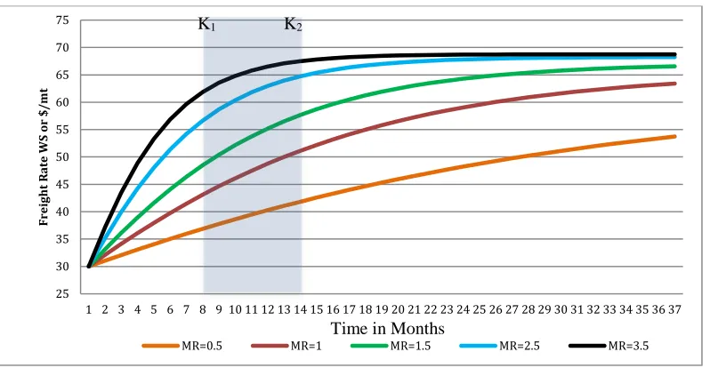
As discussed, under the assumption that operational earnings follow a mean reverting process, the expected recovery depends on the mean reversion rate, volatility and distance from the mean i.e how far (low in this case) is the freight rate from its long-run mean. In this example, we show how different speed of recovery in the form of speed of mean reversion of freight rate affects the decision to lay-up a tanker ship. We assume that the freight rate for this type of tanker follows a log mean reverting process as in equation (7) with long run mean of WS 70 points (this can be $/mt as well)2, while the current freight rate is WS 30 and volatility of 50%. Using a discretized
version of equation (11) we can estimate the expected time period for freight to reach the
recovery level, e.g. .
Given different mean reversion rates of 3.5, 2.5, 1.5, 1.0 and 0.5, the estimated time for freight earnings to reach recovery level of WS 45 are 3.5, 4, 7, 10, and 27 months, respectively. Figure 1
illustrates the expected values of freight for 5 processes with different mean reversion rates over the next 36 months. For instance, it can be seen that if there is no other shocks introduced, it can
2 The convention in the tanker market is to negotiate and contract voyage (spot) chartering of vessels on the basis of
Worldscale (WS), which is a sort of index reproduced and reported every year by the Worldscale Association (see Alizadeh and Nomikos 2009 for detailed definition and use of WS in tanker chartering).
k~
k~
k~ k~
5 4 WS
~
take 10 months for the freight rates to recover to WS45, and 16 months to reach WS 50, if we consider a mean reversion rate of 1.0; while it could take 27 month for freight rate to reach WS 45, if the mean reversion rate is 0.5. The shaded area, which covers the period between 6 and 12 months, highlights the time threshold levels of k1 and k2, considered by the shipowner as limits
for decision to keep operating, layup, or sell/scrap the vessel. For instance, if the expected recovery is sooner than k1 the ship may not be laid up, if the expected recovery is longer than k2,
the ship might be scrapped and if the expected recovery is between k1 and k2, the ship may be
laid-up. The two time thresholds can be functions of shipping company policy, cash flow situation, age of the vessel, and expected cost of lay-up. In this setting, the shipping company may decide to continue operating the vessel, for instance at slow speed, if the freight process is believed to have a mean reversion rate of 3.5, because it is expected that the rates may bounce and reach WS 45 in about 3 months. However, if the freight process shows a slower mean reversion rate (e.g. 1 or 1.5) then the recovery to WS 45 level may take 7 to 10 months, which may trigger a lay-up decision. Finally, if the freight process shows a very slow mean reversion rate, then recovery may take much longer and the shipping company may find that the cost of keeping the vessel in lay-up may exceed the benefit of having it laid-up and may well decide to sell or scrap the vessel altogether.
Having obtained the expected time for freight rate to recover and to reach a level of WS 45, for different mean reversion rates, we can calculate the discounted present value of the expected costs and benefits expressed in equation (5) to assess the decision to lay-up the vessel. Therefore, given a current freight rate of WS 30, an equivalent flat rate of $20/mt, bunker price of $550/mt, consumption of 80mt/day, and $6000/day OPEX (operating expenses), we can calculate the present value of the cumulative profit/loss from operating the vessel using the expected freight rates derived from equation (10), over the expected duration of lay-up for different mean reversion rates.
To calculate the cost of lay-up we use the present value of all the costs involved in laying-up the vessel including the initial cost of 200,000 US dollars, a variable maintenance cost of $2000/day, and a fixed expected reactivation cost of 400,000$. Assuming a fixed discount rate (e.g. 3%) we can calculate the discounted present value of the cash flow loss from keeping the vessel operational and compare it with the discounted present value of cash flow loss when the vessel is
laid-up until expected recovery time ( ) , i.e. when the freight rate reaches .
Figure 2 presents the expected cumulative cash flow from operating the vessel against the
on different levels of mean reversion rates. The threshold levels of k1 and k2 determine the loss
levels at which the company decides 1. to continue operating (lay-up period is less than k1=3
months and operating losses are less than lay-up costs) 2. lay-up the vessel when the losses from operating the vessel fall below the losses due to lay-up (lay-up period is between k1=3 and k2=7
months) or 3. sell or scrap the vessel if losses are too high (lay-up period is greater than k2=7
months and losses more than $1,000,000). As mentioned, the two time threshold levels (k1 and k2) are functions of the company’s strategy, cash flow situation, age of the vessel and customer
commitments. It can be seen that in this simulation exercise, under the assumed mean reversion rate of 0.5 the option of scrapping and selling can be considered, whereas if the mean reversion of freight rates is between 1.25 and 2.5, the option of laying up the vessel is a viable one; when the mean reversion is greater than 2.5, it might be more cost effective to keep the vessel operational, be that under slow-steaming or not.
5. Empirical Evidence
To further investigate the role of stochastic freight behaviour and of its parameters on the
decision to lay-up, we use a linear regression model with the change in laid-up tanker tonnage
(LU) as the dependent variable, and the mean reversion rate ( or MR), volatility ( or VOL),
and deviation of tanker freight rate from its long run level (-lnSt) as independent variables, in
the following form
(12)
DLM denotes the deviation of the freight rate from its long-run mean, , which serves the purpose of linking changes in the lay-up rate to the current freight rate level and the distance of
the latter from its long run average. To construct the series for volatility and mean reversion rate,
we use a long data set of monthly freight rates (January 1974 to December 2013) for VLCC
tankers serving the major route between Persian Gulf and the West Europe (Ras Tanura to
Rotterdam) obtained from Clarkson’s Shipping Intelligence Network (SIN). We estimate end of
year annualised freight volatility using an exponentially weighted average standard deviation,
while the mean reversion rate and long run mean are calculated based on the observations over
) , 0 ( ~ ;
2
1 3 2
1
0
MR DLM VOL iid
LUt t t t t t
the last 10 years.3 The lay-up data include yearly observations from 1983 to 2013 i.e. 31
observations in total. The estimation result of equation (12) is reported in Table 1. The sign of
the estimated coefficients of the mean reversion rate of freight, 1, of the distance from the long
run mean, 2, and of the volatility of tanker freight rates, 3, seem to have the expected signs
[image:16.612.102.511.225.385.2]which is consistent with the constructed model.
Table 1: Regression result of lay-up fleet on mean reversion rate, volatility and distance to mean of freight rates for tanker ships
Coefficient Standard Error T-stat p-value
0 -0.051 4.624 -0.011 0.991
1 -2.670 1.150 -2.321 0.028
2 -4.419 2.054 -2.152 0.041
3 6.766 5.182 1.306 0.203
R2 0.248
LBQ(1) 6.4299 0.011
LBQ(4) 8.0388 0.090
White 2.205 0.0652
Sample: 1983 to 2013
Heterocedasticity and Autocorrelation adjusted standard errors
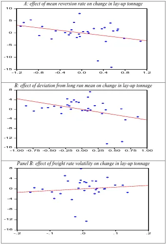
Figure presents the partial effect of the explanatory variables on the change in tanker lay-up rates
over the sample period. The partial effect can be considered as the impact of the explanatory
variable on the dependent variable, when the effects of all other factors have been taken into
account or controlled. It can be seen that when the speed of the mean reversion (MR) increases lay-up is reduced. Hence, when the expected time to recovery is shorter the expected time that a
vessel is laid-up falls and the one-time costs of laying-up become relatively more important
thereby reducing the loss preventing effect of laying-up. The effect on lay-up of the distance
from the current freight rates to their long-term mean (DLM) affects lay-up most when the distance is shorter compared to when current freight rates are further away from the long-term
3The mean reversion rate of the spot freight rate can be estimated relatively simply and robustly via linear regression. Applying Ito's lemma for Xt= ln(St), the equation (7) can be written as
where . This can be discretised as , where and
, which can be solved simultaneously to obtain and .
) , 0 ( ~ ;
2
1 3 2
1
0
MR DLM VOL iid
LUt t t t t t
dz d X dXt(* t) t )
2 / exp( 2
*
Xt01Xt1t ; t~N(0,2) t
* 0
t
mean. When the current freight rates are far below their long-term mean, scrapping the vessel
may seem a more relevant alternative than lay-up. Finally, the results also indicate that the
volatility (VOL) in the freight rates has limited effect on lay-up.
6. Conclusions and further research
The empirical investigation of the role of mean reversion in the development of freight rates
confirms - on the basis of market data - the hypothesis stated in previous research (Alizadeh et
al, 2014) that the underlying stochastic process of freight rates and the mean reversion rate,
influence significantly the decision to lay-up. In addition, the new regulatory, ever-rising, quality
standards have increased the cost of lay-up and of vessel reactivation which implies that the
freight rate threshold has been adjusted further.
The main conclusion of the paper is that faster mean reversion during the last cycle has
contributed to keeping lay-up at surprisingly low levels in a crisis context. Further research,
however, is still warranted in order to define the role of elements such as the increased
re-activation costs in the decision-making process. While the decision for each individual company
is considered to be triggered by individual factors such as its cash flow condition, age of vessel
and company strategy on fleet retention (Alizadeh et al 2014), anecdotal evidence suggests that
the role customer retention has acquired in determining tactical decisions, such as lay-up, needs
to be further investigated. Such a research direction should turn to empirical data through a
survey among shipowners to investigate their decision-making process and the criteria serving to
evaluate operational alternatives. In a further research prospect, the analysis highlighted the need
for a thorough comparison of the major shipping segments to other industries – including those
Appendix A:
Solution to Equation (9)
(A. 1)
Rearranging equation (A. 1) will result in
Simplify by setting , , , and
(A. 2)
Solving the quadratic equation with respect to X yields
(A. 3)
The final solution is
(A. 4)
) (k e X
4 2 B 2 2
C DlnSt ElnS~
S e e S e S
Et t k k t k (1 k ) ~
4 2 ) 1 ( ln exp )
( 2 ( )
2 2 ) ( ) ( 0 ~ ln 4 4 2 2 ln 2 ) ( 2 2 2 ) ( 2 ) ( S e e S
e k t k k
0
2
C CX B BX E
DX
2( )
References
Alizadeh, A. H. and Nomikos, N. K., 2009, Shipping Derivatives and Risk Management, Palgrave MacMillan.
Alizadeh, A, Strandenes, S. P., and Thanopoulou, H., 2014, Decision to Lay-up vessels under the assumption of stochastic freight rate: time-varying mean reversion and volatility, paper presented at the Proceedings of the IAME 2014 Conference, Norfolk, VA.
Balachandran, K. R., LI, S. H., and Radhakrishnan, S., 2007, A framework for unused capacity: theory and empirical analysis. Journal of Applied Management Accounting Research, 5(1), pp.21-38.
Bell, G. K. and Campa, J. M., 1997, Irreversible Investments and Volatile Markets: A study of chemical processing industry, Review of Economics and Statistics, 79 Issue 1, pp. 79-87. Bower JL. 1986. When Markets Quake. Harvard University Press: Cambridge, MA.
Brekke, K.A., and Øksendal, B., 1994, Optimal switching in an economic activity under uncertainty. SIAM Journal on Control and Optimization, 32(4), 1021–1036.
Brennan, M. J., and Schwartz, E. S., 1985, Evaluating natural resource investments. Journal of business, 58(2), pp.135-157.
Casson, M., 1997, Information and Organisation: A new perspective on theory of the firm, Oxford University Press.
Clarkson Research, 2013, Shipping Review and Outlook, http://www.clarksons.net 19/01/2014 12:45:01 83406.
Cortazar, G., and Schwartz, E. S., 1997, Implementing a real option model for valuing an undeveloped oil field. International Transactions in Operational Research, 4(2), pp.125-137. Dunford, C. and Sau, W.T., 2009, An overview of laying-up ships, CSL Presentation, Date of
access: 19/11/2013. http://www.cslglobal.com/download/download_type-68.pdf
Dixit, A., 1989, Entry and exit decisions under uncertainty. Journal of Political Economy, 97(3), 620-638
Dixit, A.K., and Pindyck, R.S., 1994, Investment under uncertainty (Princeton: Princeton University Press).
Gac, 2010. Guidelines for lay-up of ships, Date of access: 27/1/2014.
http://gac.com/upload/GAC2012/downloads/Ship%20Lay%20Up%20Guidelines%20Mar10. pdf
Gibson, R., and Schwartz, E. S., 1990, Stochastic convenience yield and the pricing of oil contingent claims. The Journal of Finance, 45(3), pp. 959-976.
Gratsos, G. A., Thanopoulou, H. A., & Veenstra, A. W. (2012). Dry Bulk Shipping. The Blackwell Companion to Maritime Economics, 11, 187
Haralambides, H. 1986, Estimation of Laid-Up Tonnage in Competitive Shipping Markets, Logistics and Transportation Review, 22(2), 184-192.
Koekebakker, S., Adland, R., and Sødal, S., 2006. Are spot freight rates stationary?. Journal of Transport Economics and Policy, 40(3), 449-472.
Lun, Y.H.V., Hilmola, O.P., Goulielmus, A. M., Lia, K. H., and Cheng, T. C. E., 2013, Oil Transport Management, VIII, Springer.
Mossin, J., 1968, An Optimal Policy for Lay-Up Decisions. Scandinavian Journal of Economics, 70(3), 170-177.
Schwartz, E. S., 1997, The stochastic behavior of commodity prices: Implications for valuation and hedging. The Journal of Finance, 52(3), 923-973.
Sridharan, S. V., 1998, Managing capacity in tightly constrained systems. International Journal
of Production Economics, 56, pp. 601-610.
Stopford, M., 2010, Shipping Market Cycles. In: Handbook of Maritime Economics and Business, 2nd edition, edited by C. Grammenos. (London: Informa), pp. 235-258.
Strandenes, S, P. 2010, Economics of the Markets for Ships In: Handbook of Maritime Economics and Business, 2nd edition, edited by C. Grammenos. (London: Lloyd’s List), pp. 217-234.
Strømme Svensden, A., 1956, Sjøtransport og skipsfartsøkonomikk (Seaborne transport and shipping economics). Samfunnsøkonomisk institutt, Norges Handelshøyskole.
Thanopoulou, H., 2010, Investing in Twenty-First Century Shipping: An Essay on Perennial Constraints, Risks and Great Expectations. In: Handbook of Maritime Economics and Business, 2nd edition, edited by C. Grammenos. (London: Lloyd’s List), pp. 659-682.
Tvedt, J., 2003, Shipping market models and the specification of freight rate processes. Maritime Economics & Logistics, 5(4), 327-346.
Von Kalckreuth, U., 2006, Financial constraints and capacity adjustment: evidence from a large
panel of survey data. Economica, 73(292), pp. 691-724.
Figure 1: Expected duration of the lay-up period for different levels of recovery under mean reversion process
Figure 2: Expected operating loss against the lay-up cost under different mean reversion rates
25 30 35 40 45 50 55 60 65 70 75
1 2 3 4 5 6 7 8 9 10 11 12 13 14 15 16 17 18 19 20 21 22 23 24 25 26 27 28 29 30 31 32 33 34 35 36 37
Fr
ei
gh
t
R
at
e
W
S
or
$
/m
t
MR=0.5 MR=1 MR=1.5 MR=2.5 MR=3.5
0 2 4 6 8 10 12 14 16 18 20
-4,500,000 -4,000,000 -3,500,000 -3,000,000 -2,500,000 -2,000,000 -1,500,000 -1,000,000 -500,000
-0.5 0.75 1 1.25 1.5 1.75 2 2.25 2.5 2.75 3 3.25 3.5
Cu
m
m
u
la
ti
ve
lo
ss
in
U
S$
Mean Reversion Rate of Freight
Cum Layup cost in US$ (LH Axis) Operating P/L in US$ (LH Axis) Time to Recovery in months (RH Axis)
K1 K2
Time in Months
Slow steam Layup
[image:21.612.98.516.367.614.2]Figure 3: The Partial effects of regressors on the change in lay-up tonnage
A: effect of mean reversion rate on change in lay-up tonnage
B: effect of deviation from long run mean on change in lay-up tonnage
Panel B: effect of freight rate volatility on change in lay-up tonnage
-15 -10 -5 0 5 10
-1.2 -0.8 -0.4 0.0 0.4 0.8 1.2
-16 -12 -8 -4 0 4 8
-1.00 -0.75 -0.50 -0.25 0.00 0.25 0.50 0.75 1.00
-16 -12 -8 -4 0 4 8