Hedging of Asian options under exponential Lévy models: computation and performance

City, University of London Institutional Repository

Citation

:

under exponential Lévy models: computation and performance. The European Journal of Finance, 23(4), pp. 297-323. doi: 10.1080/1351847X.2015.1066694

This is the accepted version of the paper.

This version of the publication may differ from the final published

version.

Permanent repository link:

Link to published version

:

Copyright and reuse:

City Research Online aims to make research

outputs of City, University of London available to a wider audience.

Copyright and Moral Rights remain with the author(s) and/or copyright

holders. URLs from City Research Online may be freely distributed and

linked to.

City Research Online: http://openaccess.city.ac.uk/ [email protected]

models: computation and performance

Laura Ballotta

, Russell Gerrard

, and Ioannis Kyriakou

1_{Faculty of Finance}

2_{Faculty of Actuarial Science and Insurance}

Cass Business School, City University London, UK

June 2015

Abstract

In this paper we consider the problem of hedging an arithmetic Asian option with

discrete monitoring in an exponential L´evy model by deriving backward recursive

inte-grals for the price sensitivities of the option. The procedure is applied to the analysis

of the performance of the delta and delta-gamma hedges in an incomplete market;

particular attention is paid to the hedging error and the impact of model error on the

quality of the chosen hedging strategy. The numerical analysis shows the impact of

jump risk on the hedging error of the option position, and the importance of including

traded options in the hedging portfolio for the reduction of this risk.

Keywords: Arithmetic Asian options, Discrete monitoring, Price sensitivities,

L´evy processes, Hedging error, Model misspecification

JEL Classification: G13, G11, D52, C63

∗_{Corresponding Author: Email: [email protected]}

1

Introduction

In this paper we investigate the problem of computing the price sensitivities of European

arithmetic Asian options with discrete monitoring, and the performance of the resulting

hedging portfolios in terms of reduction of the option’s risk exposure. To this purpose, we

derive a method for computing the option price sensitivities (like delta and gamma) and

study the impact of ignoring the probability of shocks occurring to the underlying asset

price during the contract’s lifetime.

Practitioners are interested in accurate and efficient ways to calculate the prices of

deriva-tive contracts, but also their sensitivities (also known as the ‘Greeks’) obtained by

differen-tiating the contract price with respect to parameters of interest. Common Greeks are the

so-called delta and gamma, which represent the first and second derivatives of the contract

price with respect to the value of the underlying, S0, and the vega which is given by the first derivative of the contract price with respect to the volatility of the underlying. The

Greeks are used to construct portfolios aimed at hedging the exposure originated by the

cor-responding option contract by trading in the underlying asset and/or other options. Their

appeal stems from the fact that they lead to linear hedging rules, a desirable feature in that

it allows reducing significantly the computational cost of hedging a book of options written

on the same underlying.

Asian options are derivative contracts written on the arithmetic average value of the

un-derlying which trade frequently in various markets, including the equity (e.g., see Fusai and Meucci,

2008), commodity (e.g., see Fusai et al., 2008), currency (e.g., see Lo et al., 2008) and freight

(e.g., see Nomikos et al., 2013) markets. Their appeal stems mainly from the fact that, as

the payoff depends on the average value of the underlying, the risk of market manipulations

as the contract approaches maturity is reduced. As the recent events in the financial markets

have highlighted the importance of capturing market shocks using more refined distribution

assumptions compared to the standard Black–Scholes framework, in this paper we consider

the case of an underlying asset modelled according to an exponential L´evy process, and

features on the hedging of a book of Asian options.

Exponential L´evy models generally correspond to incomplete markets due to the

intro-duction of discontinuities in the asset prices trajectories. Hedging under these conditions

presents a number of challenges. In first place, hedging can no longer be interpreted as exact

replication, like in the Black–Scholes model, but only as an approximation of the terminal

payoff offered by the contract under consideration. In this context, in fact, the classical delta

hedge is known to be sub-optimal as it does not eliminate risk completely; this implies the

introduction of a non-trivial hedging error in form of residual risk from the original exposure.

A popular alternative approach is the so-called quadratic hedging which, broadly speaking,

aims at minimizing the expected squared deviation of the hedging portfolio from the

con-tingent claim (for fuller details on quadratic hedging, we refer for example to Tankov, 2010;

Goutte et al., 2013, 2014, and references therein). However, Greeks-based hedging strategies

like, for example, delta and delta-gamma hedges are still commonly used in practice; in

particular, the delta hedge is shown to generate an error which is relatively close to the one

produced by quadratic hedging (see Denkl et al., 2013; Cont et al., 2007, amongst others).

For the case of a discretely sampled Asian option, an additional challenge is due to the lack

of analytical solution for the contract price, and hence its sensitivities.

Over the last few years fast and accurate algorithms emerged for pricing European

discrete arithmetic Asian options beyond the traditional lognormal asset price model; we

mention, amongst others, ˇCern´y and Kyriakou (2011), Fusai and Meucci (2008), Fusai et al.

(2008), Fusai et al. (2011), Marena et al. (2013) and Zhang and Oosterlee (2013). Whereas

the pricing of Asian options is well-understood, an additional interesting direction to

ex-plore is that of the computation of the price sensitivities, which poses the main challenge of

proving validity of the interchange of differentiation and the integral price representation.

In light of the previous discussion, the contribution of our paper is two-fold. Firstly, we

develop a method for computing the price sensitivities of the European Asian option using

backward recursive convolutions. In more details, our approach is based on direct

differenti-ation of the risk neutral conditional expectdifferenti-ation of the discounted payoff of the Asian option

generic process with independent increments for the log-returns of the underlying, we prove

that differentiation under the integral sign with respect to parameters of interest is

permis-sible. In particular, we reach general solutions for the option’s delta and gamma (Theorem

1), but also the non-trivial case of the option’s vega for a lognormal underlying (Theorem

2); en route, we prove that the vega of the given contract is positive, extending the results

of Carr et al. (2008) from the case of a continuously to a discretely monitored arithmetic

Asian option. It is worth pointing out that the suggested method can give access to any

other price sensitivity, providing that differentiation under the integral sign is allowed. The

accuracy of our method is demonstrated by numerical tests performed under different L´evy

models for the asset log-returns, like the Brownian motion, the Normal Inverse Gaussian

(NIG) model (Barndorff-Nielsen, 1995) and the Carr–Geman–Madan–Yor (CGMY) model

(Carr et al., 2002); we also provide a comparison against the outcome from Monte Carlo

simulations. Secondly, we use the proposed method to set up the delta and delta-gamma

hedging portfolios for the Asian option under consideration, and investigate their

perfor-mance in the incomplete market originated by the adopted exponential L´evy models. In

particular, we pay attention to the goodness of the approximation of the terminal payoff of

the contract and the behaviour of the residual risk, i.e. the hedging error. We also study

the impact of misspecifying the underlying asset price dynamics on the performance of the

Greeks-based hedging portfolios, which we refer to as model error.

The outline of the paper is as follows. In Section 2 we present our main theoretical

findings on the computation of the price sensitivities of Asian options. In Section 3 we

present the results from the numerical implementation of the proposed method; the procedure

is benchmarked against Monte Carlo (with control variate). In Section 4 we illustrate the

performance of Greeks-based hedges (like the delta and delta-gamma portfolios) in terms

of hedging error and model error. Section 5 concludes. All the proofs are deferred to the

2

Recursive integrals for Asian option sensitivities

2.1

Backward price recursion

Consider an Asian option with underlyingSobserved over the period (0, T] at the equidistant

times t1 = δ, t2 = 2δ, . . . , tn =nδ =T. Let {Zk}nk=1 be a collection of independent random variables representing the log-returns onS, such that

Sj =S0exp(

Xj

k=1Zk), j = 1, . . . , n, S0 >0.

The sequence _{Zk}nk=1 can be thought of, for example, as the increments of a specific L´evy process, such as the Brownian motion, the NIG process or the CGMY process.

Under the unified framework of Veˇceˇr (2002), the payoff of an Asian option is generally

given by

(Xn

k=0λkSk)

+_{, (1)}

where (_·)+ _{is the positive part function and coefficients {λ}

k}nk=0 are deterministic and take different values for different contract specifications. For example, for

λ0 :=−

K S0

and λk := 1

n, 0< k≤n, (2)

we retrieve the payoff of the call option with fixed strike priceK >0

(Xn

k=1λkSk) +₌

1

n

Xn

k=1Sk−K

+

.

Define the reverse filtrationG_={Gk}n

k=1 forGk =σ{Zn, Zn−1, . . . , Zn+1−k}, and consider the process

Yk = ln(eYk−1 +λn+1−k) +Zn+1−k, 1< k ≤n, (3)

withλk >0, 0< k ≤n. On evaluating exp(Yk) recursively using (3)–(4), we can factorize (1)

as S0(eYn+λ0)+, whereλ0 ∈R. (This factorization result has been contributed by Stewart Hodges and first appeared in Carverhill and Clewlow, 1990.)

Without loss of generality, we focus here on the call option with fixed strike price satisfying

(2). Then, given the price of the fixed strike call, the price of the floating strike put option can

be obtained using a symmetry relationship derived in Eberlein and Papapantoleon (2005) for

underlyings driven by exponential L´evy models, while the prices of the fixed strike put and

floating strike call options can be obtained via standard put-call parity (e.g., see Fusai et al.,

2011).

As the processY is Markov in the filtrationG_{, the forward price of the optionE((S0e}Yn₋ K)+_{) under some risk neutral measure P can be computed recursively on a one-dimensional} grid. To this end, assume that for all k the random variables Zn+1−k have density functions

fk. For any S0 >0 and fixed K >0, define

pn(y) =S0(ey +λ0)+ = (S0ey−K)+. (5)

Further, define recursively

˜

pk−1(x) =

Z ∞

−∞

pk(x+z)fk(z)dz, 0< k ≤n, (6)

pk(y) = ˜pk(hk(y)), 0< k < n, (7)

where

hk(y) = ln(ey+λn−k), 0< k < n. (8)

It is shown in ˇCern´y and Kyriakou (2011, Theorem 3.1) that

0 _≤ pk(y)≤ak+bkey, (9)

where

an = 0, bn=S0, (11)

ak = ak+1+bkλn−k, bk =bk+1µk+1 (12)

for

µk :=E(eZn+1−k) =

Z ∞

−∞

ezfk(z)dz <∞.

The forward price of an Asian call option with coefficients _{λk}as in (2) is given by

E((S0eYn−K)+) = ˜p0(lnλn). (13)

2.2

Delta and gamma recursions

In this section we show that, by direct differentiation of the risk neutral valuation formula

(13) with respect to the initial asset value S0, we are able to derive backward recursive convolutions that produce the exact Asian call option’s delta and gamma sensitivities. For

this to be feasible, we need first to guarantee differentiation under the integral sign. These

results are proved in the following.

Theorem 1 Assume S0 lies on a bounded interval of the positive real axis. Suppose that,

in addition to µk < ∞, µ¯k := E(e−Zn+1−k) = R_−∞∞ e−zfk(z)dz < ∞ for all k. Consider the

sequence of functions (5)–(8). The following statements hold. (i) There exists a sequence of non-negative constants given by

αn = 0, βn = 1,

αk = αk+1+βkλn−k, βk =βk+1µk+1,

such that

0 _≤ ∂

∂S0

pk(y;S0)≤αk+βkey for k≤n, (14)

0 _≤ ∂

∂S0 ˜

for all y and x. (ii) For k_≤n₋1,

∂2

∂S2 0

pk(y;S0),

∂2

∂S2 0

˜

pk(x;S0)≥0

for all y and x.

Further, there exists a sequence of non-negative constants given by

γn−1 = −

λ0

S0

, εn−1 =−

λ0λ1

S0

, ζn−1 = 0, ηn−1 = 0,

γk = γk+1+ζk+1µk+1λn−k,

εk = εk+1µ¯k+1+ (γk+1+ηk+1)λn−k+ζk+1µk+1λ2n−k,

ζk = ζk+1µk+1,

ηk = ηk+1+ζk+1µk+1λn−k,

such that over any compact interval y_∈[L, U] _⊂R

Z U

L

∂2

∂S2 0

pk(y;S0)dy≤γk+εke−L+ζkeU+ηkeU−L for k ≤n−1. (15)

(iii) There exists a sequence of functions given by

∂ ∂S0

pn(y;S0) = ey1y>ln(−λ0),

∂2

∂S2 0

pn−1(y;S0) = −

λ0

S0

fn

ln

−_eyλ₊0_λ

1

and

∂j

∂S₀jp˜k−1(x;S0) =

Z ∞

−∞

∂j

∂S₀jpk(x+z;S0)fk(z)dz, (16) ∂j

∂S0j

pk(y;S0) =

∂j

∂S0j ˜

pk(hk(y);S0)

option are given by

∂j

∂S₀jp˜0(lnλn;S0)

for j = 1 and 2, respectively.

Proof. See Appendix A.

2.3

Vega recursion

In this section the Black–Scholes model is assumed, i.e. the log-returns _{Zn+1−k} represent the increments of a Brownian motion with drift, and therefore are identically distributed and

follow a normal distribution with meanE(Z) = (r₋σ2_{/2)δand variance Var(Z) =σ}2_{δ, where}

r and σ denote the continuously compounded risk free rate of interest and the volatility of

the underlying, respectively. We derive the recursive convolution for the Asian call option’s

vega, i.e. the Greek with respect to the model-specific parameter σ. Similarly to the case

presented in Section 2.2, we need to guarantee that direct differentiation of (13) is feasible.

We note that, whereas the convolutions of Section 2.2 rely on the dependence of the terminal

payoff function (5) on S0, additional complexity emerges in the case of the vega due to the dependence of the log-returns probability density f onσ at every iteration.

Our result is tailored to normal distributed log-returns. However, providing that the

interchange between integration and differentiation in (6) is permitted, similar recursions

can be obtained for sensitivities with respect to parameters of other L´evy models for the

log-returns, including, for example, the volatility parameters ν and γ of the NIG model

(see Bayazit and Nolder, 2013; Corcuera et al., 2008) with characteristic exponent (19), or

market parameters, like the risk free rate r (so-called rho sensitivity). Mixed sensitivities,

for example, with respect to the initial asset value and volatility (so-called vanna sensitivity)

can also be obtained. Additional results can be made available by the authors upon request.

Theorem 2 Let σ be the volatility of the price of underlying in the Black–Scholes model.

(i) There exists a sequence of non-negative constants given by

˜

cn−1 = 0, dn−1 = 1

√

2πS0

√

δerδ, cn−1 =dn−1λ1,

˜

ck = ck+1+ak+1

1

σ +

1 4σδ

,

dk = dk+1+bk+1

1

σ +

1 4σδ

,

ck = ˜ck+dkλn−k,

where the constants ak, bk are given by (11)–(12), such that

0 _≤ ∂

∂σp˜k(x;σ)≤˜ck+dke

x

0 _≤ ∂

∂σpk(y;σ)≤ck+dke

y ₍₁₇₎

for 0< k_≤n₋1, for all x and y.

(ii) There exists a sequence of functions given by

∂

∂σpn−1(y;σ) =S0

√

δerδ(ey+λ1)φ

ln(₋ey+λ1

λ0 ) + (r+ 1 2σ

2_)δ

σ√δ

!

,

where φ is the standard normal density function, and

∂

∂σp˜k−1(x;σ) =

Z ∞

−∞

∂

∂σpk(x+z;σ)f(z;σ) +pk(x+z;σ) ∂

∂σf(z;σ)

dz, (18)

∂

∂σpk(y;σ) = ∂

∂σp˜k(hk(y);σ),

where f(z;σ) := φ(z₋(r₋ 1 2σ

2_)δ)/(σ√_δ)/(σ√_{δ). The forward vega of the Asian}

call option is given by

∂

∂σp˜0(lnλn;σ).

Proof. See Appendix B.

We note that the vega of the given contract is always positive (see Equation 17), which

Asian option.

3

Algorithm performance analysis

3.1

Implementation

For illustration purposes, we test the backward integral recursions for the delta and gamma

in the case in which the log-returns of the underlying asset are governed by a L´evy process;

specifically we consider the case of a Brownian motion with drift (standard Black–Scholes

(BS) model), the NIG process and the CGMY process. The corresponding characteristic

functions are

E(eiuZk_{) = e}ψ(u)δ_{, ∀k,}

ψ(u) = iu(r₋ψˆ(₋i)) + ˆψ(u),

where

ˆ

ψBS(u) = ₋1

2σ

2_u2_{, σ >0,} ˆ

ψNIG(u) = 1

ν(1−

p

1₋2iθνu+νγ2_u2_{), θ∈R, ν, γ >0, (19)}

ˆ

ψCGMY(u) = CΓ(₋Y)((M₋iu)Y ₋MY + (G+iu)Y ₋GY), C, M, G >0, Y <2.

We also analyze the case of the vega sensitivity in the Black–Scholes model.

We compute numerically the Greeks convolutions (16) and (18) by Fourier transform;

this allows us to translate the density-based solutions to characteristic function-based ones

which are faster to compute and rely on simpler expressions of characteristic functions as

op-posed to likely complicated (if available in closed form) density functions. More specifically,

we refer to Theorem 3.2 and Section 4 of ˇCern´y and Kyriakou (2011), respectively, about

the construction of the Fourier transforms and their discretization for a fast numerical

im-plementation using the so-called chirp z-transform (see also Bluestein, 1968; Rabiner et al.,

plat-forms like Matlab. This powerful approach allows us to gauge explicitly the precision of the

scheme and, by further exploiting its smooth convergence in the number of discretization

points of the Fourier transforms, achieve highly accurate results as we show in the following

section. Alternatively, one may consider using the maturity randomization algorithm

pre-sented in Fusai et al. (2011) or the parallel wavelet-based procedure of Corsaro et al. (2015)

for potential speed-up gains with increasing monitoring frequency. Richardson extrapolation

techniques also provide substantial CPU power saving when dealing with a large number of

monitoring dates.

As a benchmark, we use the results from Monte Carlo simulations. In particular, we

employ classical pathwise (PW) estimation for the delta and vega (see Curran, 1994, 1998;

Broadie and Glasserman, 1996, for example). In the case of gamma, we use mixed likelihood

ratio-pathwise (LRPW) estimation (i.e. utilize each of the LR and PW approaches for one

order of differentiation) which induces lowest standard error (see Glasserman, 2004). The

latter case requires access to the density function of the log-returns, which in the case of the

NIG and CGMY distributions we retrieve by transform inversion as in Glasserman and Liu

(2010). In addition, given the characteristic function of the log-geometric average which has

been derived in Fusai and Meucci (2008) for general independent and identically distributed

(i.i.d.) log-returns, one can compute geometric option sensitivities at high accuracy using,

for example, the inverse-transform formula of Carr and Madan (1999). This allows us to

use the geometric option sensitivities as control variates in the estimation of the arithmetic

option sensitivities. Finally, we simulate the NIG process using its subordinated Brownian

motion representation (e.g., see Glasserman, 2004), while for the CGMY dynamics we adopt

the joint Monte Carlo-Fourier transform sampling scheme in Ballotta and Kyriakou (2014)

based on direct simulation of the process increments.

Results are shown in the following section.

3.2

Results

We opt for Asian call options with fixed strikes K =_{90,100,110_}, time to maturityT = 1,

free rate r = 0.04. For illustration purposes, we use the calibration (to stock index option

prices) results of ˇCern´y and Kyriakou (2011) to achieve target volatility Vol =_{0.1,0.3,0.5_}

for all models, in addition to a skewness coefficient of₋0.5 and excess kurtosis of 0.7 for the

NIG and CGMY models, see Panel (a) of Table 1.

In Panel (b) of Table 1, we list the numerical results for the Greeks of arithmetic Asian call

options from the backward recursions implemented using the transform technique referred to

in Section 3.1 and the control variate Monte Carlo (CVMC) simulations (we employ standard

CVMC setup with the CV coefficient estimated using a pilot run, as detailed, for example, in

Glasserman, 2004). Across strikes, models and volatility levels, we observe smooth monotone

convergence in the number of discretization points of the integral recursions, similarly to

ˇ

Cern´y and Kyriakou (2011). We present results with accuracy to 6 decimals achieved in up

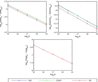
to 1.5 seconds1_{, which is sufficient for the purposes of our hedging strategy exercise in Section} 4. By sake of exemplification, in Figure 2 we present on a log-log scale the convergence

patterns of the computed deltas and gammas in the NIG, CGMY and Black–Scholes models

and vegas in the Black–Scholes model for an at-the-money option (i.e., S0 = K = 100) and the case of volatility Vol = 0.1 (see Panel (a) of Table 1). We observe that smoothly

diminishing error patterns are preserved under both leptokurtic or normal log-returns which

ensure convergence to the desired number of decimal places reported on the left side of

Panel (b) of Table 1. These can be exploited to achieve even higher accuracies, e.g., up

to 10 decimals, with minimal extra computational cost (up to 4 seconds) using Richardson

extrapolation (e.g., see Andricopoulos et al., 2003). (More numerical results are available

upon request by the authors.) We note that all computed Greeks using backward recursions

fall into the 99% confidence intervals estimated using 100,000 Monte Carlo simulations. To

further demonstrate the power of our approach, we compute (proofs are omitted) backward

recursions for the sensitivities with respect to the volatility parameters ν and γ of the NIG

model log-returns (see discussion in Section 2.3) as well as the mixed sensitivity with respect

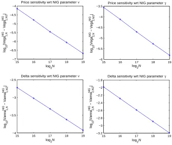
toS0and the volatility parametersνandγ (vanna sensitivity). Figure 3 presents on a log-log scale smoothly diminishing error patterns of the computed sensitivities for an at-the-money

option (i.e., S0 = K = 100) and the case of Vol = 0.1 (see Panel (a) of Table 1). In this example, with 6-decimal-place accuracy, the vega wrt ν is 1.673078; wrt γ is 17.567563,

whereas the vanna wrt ν is 0.142703; wrt γ is₋1.263555.

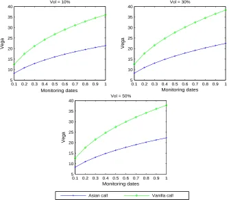
In the case of vega, the performance of Monte Carlo simulation deteriorates generating

vega estimates with high standard errors, whereas the backward convolution method remains

consistently accurate and efficient. Given our highly precise results for the vega of the Asian

option, it is then easy to verify that, across strikes and volatilities, these are consistently

lower than the ones of the corresponding plain vanilla option which can be seen as a special

case of the Asian option with a single monitoring date. Figure 1 shows the case of

at-the-money options with different maturities and for different volatility levels. This confirms the

lower sensitivity of the contract to the volatility of the underlying asset induced by averaging,

which explains the interest of investors for this type of option.

4

Hedging strategies performance analysis

In the following we consider the problem of hedging the given arithmetic Asian call option

contract using the option’s Greeks computed with the scheme proposed in Section 2.

We begin by noting from the results reported in Panel (b) of Table 1 the difference

between the values of delta and gamma obtained under the Black–Scholes model and the

ones generated by the NIG and the CGMY processes, which can reach up to 24% in the

case of delta and 20% in the case of gamma. On the other hand, the estimates of these two

sensitivities are very close under the NIG and the CGMY, which is consistent with intuition

given that the first four cumulants of the log-returns distribution are matched under the

chosen parameters values. In this respect, we conclude that model error is less severe when

shocks are incorporated, even if this might be done sub-optimally, i.e. by choosing for

example an infinite variation process such as the NIG instead of a finite variation one such

as the CGMY considered in this example (note the choice of Y = 0.8 _∈ (0,1)). Hence, for

ease of exposition, in the remaining of this section we focus on the case of the NIG model

for the analysis of the performance of Greeks-based hedging strategies in presence of jumps

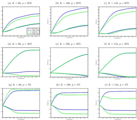
The numerical experiment is in spirit similar to the one carried out in Yang et al. (2011)

and is organized as follows. We generate 1,000 batches of 10,000 NIG trajectories monitored

at the reset dates of the Asian option; for each batch we select those trajectories generating

the 5% (‘worst’ case scenario), the 50% (the median) and the 95% (‘best’ case scenario)

quantile of the arithmetic average price of the underlying entering the terminal option payoff.

Along the selected quantile trajectories, we compute the option’s delta and gamma over the

contract term using the backward integral recursion presented in Section 2.2; results are

presented in Section 4.1. Finally, the previously computed Greeks are used to construct the

delta hedging portfolio and the delta-gamma hedging portfolio of the Asian option for the

strikes and the volatility values considered in Section 3.2. As the market is incomplete and

exact replication is not possible, hedging can only be interpreted as an approximation of the

terminal payoff, and as such it leads to the introduction of non-trivial error. We analyze this

hedging error in Section 4.2.

In order to study model error as well, i.e. the error originated by the fact that the

hedge may be derived in a model differing from the one where it is eventually applied,

we use the backward integral recursion developed in Section 2.2 to compute the delta, the

gamma and the corresponding hedging portfolios of the Asian option also under the Black–

Scholes economy, and compare their performance over the lifetime of the contract to the

ones obtained under the NIG model. The analysis is presented in Section 4.3.

Finally, we note that the rebalancing of the hedging portfolio is performed at the

mon-itoring dates of the Asian call option; this choice is motivated mainly by the attempt to

conciliate the trade-off between accuracy of the hedging position (which from the theoretical

point of view requires continuous rebalancing) and the transaction costs which the trader

would incur by frequently re-adjusting the portfolio. For a detailed analysis of the error

originated by discrete rebalancing as the one adopted in our analysis, we refer for example

to Brod´en and Tankov (2011) and Gobet and Makhlouf (2012).

In the remaining of this section we use the same parameters as in Section 3.2, which are

4.1

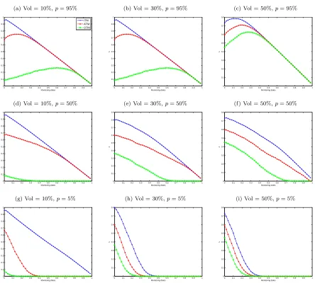
Delta and gamma

The Asian call option delta is shown in Figure 4; it represents the rate of change of the

option premium when the underlying asset price changes, and the number of shares required

to maintain the overall traders’ position delta neutral. The corresponding Asian call option

gamma is shown in Figure 5; it represents the rate of change of the delta with respect to the

underlying price, and therefore ‘quantifies’ the curvature of the option premium with respect

to the price of the underlying. Gamma neutral positions in a convex hedging instrument

(generally another option contract) are proportional to the gamma of the Asian contract.

Consistent with intuition, Figure 4 shows that, regardless of the quantile trajectory

con-sidered, the delta of the Asian call option depends on the moneyness of the contract: the

more in-the-money the option, the higher the value of the delta. This reflects the probability

of a non-zero payout at maturity from the option, and therefore determines the amount of

underlying asset the traders require to hedge their position. Figure 4 also shows that, in

gen-eral, the behaviour of the delta of in-the-money options does not change significantly across

the different quantile scenarios; the deltas of at-the-money and out-of-the-money contracts

are instead more sensitive to the underlying asset trajectory, as confirmed by the

corre-sponding values of their gamma. Figure 5 in fact shows that, especially in correspondence

of low volatility values, the gamma reaches its maximal value for at-the-money and

out-of-the-money options; on the other hand, in-out-of-the-money contracts are relatively insensitive to

second-order effects of changes in the underlying value.

In light of these results, we expect delta hedging portfolios to provide the required cover

for in-the-money options, and to require instead frequent rebalancing aimed at reducing

the residual risk in the case of at/out-of-the-money contracts. Hence, we also expect

delta-gamma hedging portfolios to be more effective for these options.

Further, the delta, in general, decreases over the lifetime of the contract, i.e. at each reset

date the traders unwind part of their delta position due to the combined effect of the weight

of the setting (see de Weert, 2008, for example) and the reduction of the uncertainty about

the terminal payoff. These results are consistent with the findings obtained for the standard

position in the risky asset is seemingly linear especially for in-the-money options. We observe

a similar feature in our case as well but only for low volatility levels of the underlying (see

Panels 4a, 4d and 4g). Similarly, the gamma decreases to zero as we approach the maturity of

the contract: the position in the hedging option is gradually liquidated, although the decay

rate changes significantly across strikes, quantile trajectories and volatility levels to take full

account of the convexity effect. In this respect, Figures 4 and 5 provide some information

about the charm and the color of the Asian call option (i.e. the delta and gamma decay,

e.g., see Garman, 1992).

Both delta and gamma are sensitive to the value of the underlying volatility used to

calculate them (these sensitivities are formalized by the so-called vanna and zomma, e.g.,

see Webb, 1999). In particular, ceteris paribus, increasing the volatility increases the delta

of out-of-the-money options, as the probability that the contracts might move in the money

increases as well. We also note that the delta of in-the-money options loses the seemingly

linear decay over time. Higher volatility levels produce generally lower gamma values (note

the scale in the panels of Figure 5): the position in the hedging option is more conservative

in more volatile market conditions.

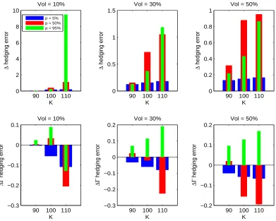
4.2

Hedging error

We define the hedging error as the difference between the hedging portfolio at maturity and

the arithmetic Asian call option’s terminal payoff, expressed as a percentage of the (forward)

option price. We compute this error in correspondence of all strikes, volatility values and

quantile trajectories considered so far; results are shown in Figure 6.

In details, the top three panels of Figure 6 illustrate the hedging errors originated by the

model delta portfolio, composed of delta units of the underlying asset and the investment in

the risk free bond, for the given three volatility levels. Each panel shows the errors for the

given moneyness levels and quantiles. The bottom three panels correspond instead to the

hedging error originated by the model delta-gamma portfolio, obtained by combining the

underlying asset and one European vanilla call option (in addition to the position in the risk

position. The vanilla option used for the gamma hedge has the same underlying asset as the

arithmetic Asian call option; we choose a contract with slightly longer maturity (the vanilla

option has maturity of 14 months, as opposed to the 12 months term of the Asian option) as

to guarantee the hedging position at least until the expiration of the Asian contracts under

consideration. Both delta and delta-gamma portfolios are rebalanced at each monitoring

date according to the current (re-computed) values of the options’ delta and gamma.

Consistently with our observation in Section 4.1, we note from Figure 6 that the hedging

errors achieve their lowest level for in-the-money options; both hedging strategies perform

poorly for out-of-the-money options, and this is particularly evident for the delta hedge of

the out-of-the-money option in the low volatility case (top left corner panel). In this case, in

fact, the hedging error can reach up to about 9 times the (forward) option’s premium, whilst

the one originated by the delta-gamma portfolio is around 12%. However, the delta-gamma

strategy always outperforms the delta portfolio by reducing the hedging error on average by

more than 70% (we note the scale of the plots in Figure 6). The most significant reduction

occurs for high volatility levels; for each volatility value, the improvement of the performance

is particularly noticeable in correspondence of the median trajectory. This shows that the

introduction of options in the hedging portfolio allows achieving an acceptable performance

even in presence of jumps, as it reduces the residual risk and its sensitivity to different

scenarios (represented by the different quantile trajectories), in spite of a more conservative

option position in the delta-gamma hedge as observed in Section 4.1 in correspondence of high

volatility conditions. This feature is in a sense consistent with the market incompleteness

caused by discontinuities in asset prices, meant as the impossibility of replicating any option

by trading in the underlying asset alone, and the need of ‘completing’ the market with

derivative instruments whose price encapsulates information about the jump risk premium.

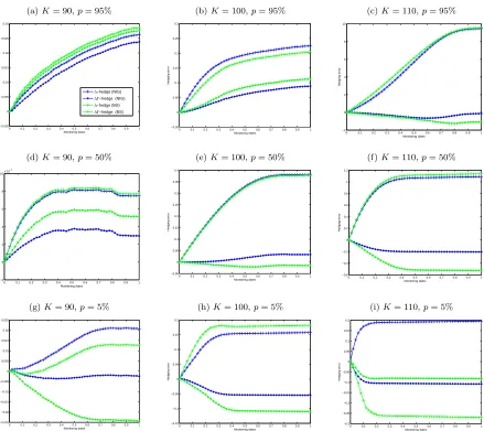
4.3

Model error

In order to quantify the error originated by model misspecification, we compare the

per-formance of the delta and delta-gamma hedging portfolios formed using the Asian option’s

ones constructed using the contract’s Greeks computed under the Black–Scholes model, i.e.

the case of the Brownian motion with drift (Black–Scholes hedging portfolios). The volatility

parameter in the Black–Scholes model is set so that the log-return processes show the same

variance under both the Gaussian and the NIG models. In other words we assume that, just

after the price of the underlying asset is revealed, the traders re-adjust their position

accord-ing to the values of the Asian option’s Greeks obtained usaccord-ing the Black–Scholes model, due to

the fact that they cannot observe directly the actual process originating the underlying asset

prices (which in this example is assumed to be the exponential NIG process). The

delta-gamma portfolios composition is the same as in the previous section. Results are presented

in Figures 7–9, in which we plot the evolution of the hedging errors originated by both the

model and the Black–Scholes hedging portfolios over the given contract’s term. Due to our

construction of the hedging error, we interpret the difference between these hedging errors as

model error, as it actually quantifies the difference between the hedging portfolio values

ob-tained under the two model specifications (divided by the forward option’s premium, which

is assumed to be the same for both models as if directly observed in the market).

We note from the plots that the Black–Scholes delta hedge consistently originates a

smaller hedging error than the model delta hedge, especially for high level of volatility

of the underlying. The portfolios are however almost undistinguishable along the median

trajectories (see Panels 7d–7f, 8d–8f and 9d–9f): over the contract’s term, the difference

between the hedging errors of the model and the Black–Scholes portfolios, in fact, ranges

on average between 0.84% and 1.43% of the (forward) option’s premium. In the case of

the ‘extreme’ trajectories, though, these differences can vary between 10% and 67%. These

results are consistent with the findings of Denkl et al. (2013).

In any case, the hedging errors are quite significant also under the Black–Scholes model:

over the lifetime of the contract, these vary on average between 0.68% to almost 10 times

the (forward) option’s price when the underlying volatility is set at 10%; the error range

narrows to 10%-98% on average for the 30% volatility case, and 9%-95% on average for the

50% volatility case.

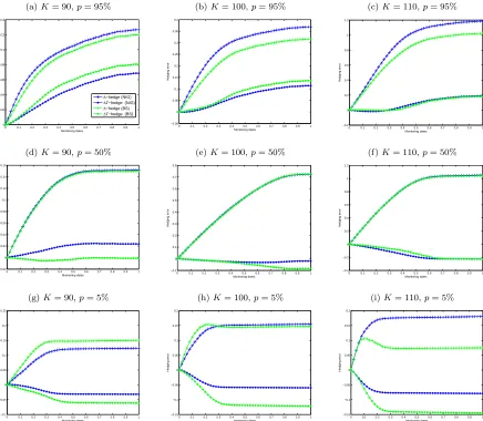
better than the delta ones reducing sensibly the hedging errors; in this case, though, the

model delta-gamma hedge performs consistently better than the Black–Scholes one, due to

the ability of the relevant sensitivities to adequately capture the impact of potential price

shocks. Model error is actually substantial across all strikes, scenarios and volatility

lev-els considered in this analysis, as the difference between the model and the Black–Scholes

delta-gamma hedging portfolios varies on average between 22% and around 6 times the

op-tion’s (forward) premium over the lifetime of the contract. The hedging error originated by

the Black–Scholes portfolios, though, reduces in the case of high volatility: as the skewness

and excess kurtosis of the NIG distribution are kept constant, the impact of jumps reduces.

Hence, the performance of the hedging portfolios obtained under the two alternative

mod-elling assumptions is comparable as the variance is the predominant component requiring

accurate quantification.

5

Conclusions

In this paper, we have derived backward integral recursions for the price sensitivities of

arithmetic Asian options with discrete monitoring. In particular, we have proved the cases

of the option’s delta and gamma for an underlying that evolves according to a general

exponential L´evy process, and the option’s vega for a lognormal underlying; however we

note that similar recursive integrals may be obtained for other price sensitivities of practical

relevance. Numerical examples show the high accuracy of the proposed approach across

different distribution laws for the log-returns, parameter values, strike prices and sensitivity

types.

The price sensitivities have been then used to assess both the performance of

Greeks-based hedging strategies in an incomplete market, and the impact of model error. We find

that the delta-gamma hedge is superior to the delta hedge in terms of reduction of the risk

exposure; further incorrectly specifying the underlying price dynamics leads to non-trivial

error which can be significant especially in the case of the delta-gamma hedge.

The presence of jumps in the dynamics of the underlying asset, the inclusion of the

from earlier contributions by Jacques (1996) and Yang et al. (2011). Future research is

di-rected at extending the analysis by comparing the quadratic hedging strategies of Cont et al.

(2007) with the delta-gamma hedge and assessing the hedging error under different market

conditions in terms of volatility, skewness and excess kurtosis.

Acknowledgements

We thank Aleˇs ˇCern´y for his contribution to a previous version of this paper. Further thanks

go to Gianluca Fusai, Olaf Menkens, Antonis Papapantoleon and Steven Vanduffel for fruitful

discussions. This paper has been presented at the 17th _{International Congress on Insurance:}

Mathematics and Economics (IME 2013). We thank all the participants for their helpful

feedback. Usual caveat applies.

Appendix A Proof of Theorem 1

Proof of (i). The proof proceeds by backward induction on k. For k =n, we have from

(5) that 0 _≤ ∂

∂S0pn(y;S0) = e y₁

y>ln(−λ0) ≤ ey. Therefore, _∂S∂0pn(y;S0) is dominated by an integrable function over compact intervals and from (6) we get that

∂ ∂S0

˜

pn−1(x;S0) =

Z ∞

−∞

∂ ∂S0

pn(x+z;S0)fn(z)dz, (A.1)

which is non-negative. Further,

∂ ∂S0

˜

pn−1(x;S0)≤

Z ∞

−∞

ex+zfn(z)dz =µnex =αn+βn−1ex.

It follows from (7) that

0_≤ ∂

∂S0

Now suppose that (14) holds for arbitrary k < n. Then the function _∂S∂₀pk(y;S0) ≥ 0 is integrable over compact intervals. As fk ≥0, we get

0 _≤ ∂

∂S0 ˜

pk−1(x;S0) =

Z ∞

−∞

∂ ∂S0

pk(x+z;S0)fk(z)dz (A.2)

≤

Z ∞

−∞

(αk+βkex+z)fk(z)dz =αk+βk−1ex

and

0_≤ ∂

∂S0

pk−1(y;S0)≤αk+βk−1λn+1−k+βk−1ex =αk−1+βk−1ey.

Proof of (ii). From (A.1), _∂S∂22

0p˜n−1(x;S0) is well-defined and is given by

∂2

∂S2 0

˜

pn−1(x;S0) =−

λ0

S0

fn(−x+ ln(−λ0))≥0.

In addition, from (7)

∂2

∂S2 0

pn−1(y;S0) = −

λ0

S0

fn(−ln(ey+λ1) + ln(−λ0))≥0,

so that Z U L ∂2 ∂S2 0

pn−1(y;S0)dy=−

λ0 S0 Z U L fn ln

−_eyλ₊0_λ

1

dy=₋λ0

S0

Z U′

L′

1 1 +λ1ew/λ0

fn(w)dw,

whereL′ _{:= ln(−λ}

0/(λ1+eU)) and U′ := ln(−λ0/(λ1+eL)). Asw≤U′, λ0 <0 and λ1 >0, it follows that 1/(1 +λ1ew/λ0)≤1 +λ1e−L and

Z U

L

∂2

∂S2 0

pn−1(y;S0)dy ≤ −

λ0(1 +λ1e−L)

S0

Z U′

L′

fn(w)dw

≤ −λ0(1 +λ1e−

L₎

S0

=γn−1+εn−1e−L,

which is finite for finite L. Hence, the statement is true for k = n ₋ 1. Now suppose

the statement is true for arbitrary k < n₋1. Therefore the function _∂S∂22

integrable fory in a compact interval, and from (A.2) we get

0_≤ ∂ 2

∂S2 0

˜

pk−1(x;S0) =

Z ∞

−∞

∂2

∂S2 0

pk(x+z;S0)fk(z)dz

and from (7)

0_≤ ∂ 2

∂S2 0

pk−1(y;S0) =

∂2

∂S2 0

˜

pk−1(ln(ey+λn+1−k);S0).

Then, Z U L ∂2 ∂S2 0

pk−1(y;S0)dy =

Z U L Z ∞ −∞ ∂2 ∂S2 0

pk(ln(ey+λn+1−k) +z;S0)fk(z)dzdy

=

Z ∞

−∞

fk(z)

Z z+ln(eU+λn+1−k)

z+ln(eL_+λ

n+1−k)

∂2

∂S2 0

pk(w;S0)

1

1₋λn+1−kez−w

dwdz.

Asw_≥z+ ln(eL_+λ

n+1−k) andλn+1−k >0 fork < n−1, we have that 1/(1−λn+1−kez−w)≤ 1 +λn+1−ke−L leading to

Z U

L

∂2

∂S2 0

pk−1(y;S0)dy ≤ (1 +λn+1−ke−L)

Z ∞

−∞

fk(z)

Z z+ln(eU+λn+1−k)

z+ln(eL_+λ

n+1−k)

∂2

∂S2 0

pk(w;S0)dwdz

≤ (1 +λn+1−ke−L)

Z ∞

−∞

γk+εk

e−z

eL_+λ n+1−k +ζkez(eU +λn+1−k) +ηk

eU _+λ n+1−k

eL_+λ n+1−k

fk(z)dz,

which is finite for finite L, U. Result (15) follows by straightforward integration.

Proof of (iii). Follows from the proofs of parts (i)–(ii) of the Theorem. This concludes

the proof of the Theorem.

Appendix B Mathematical analysis towards proving Theorem 2

We begin the path to proving Theorem 2 by providing some necessary results.

Lemma 3 There exists sequence of positive constants given by

An=S0, Ak =Ak+1(e−(r−σ 2_)δ

such that

pk(y) ≤ Ake|y| for k ≤n, ˜

pk(x) ≤ Ak+1(e−(r−σ 2_)δ

+erδ)e|x| for k < n,

for all y and x.

Proof. From (5) we have that pn(y) ≤ S0e|y|. The proof proceeds by induction. Assume

that pk(y)≤Ake|y| holds for arbitraryk < n. Then from (6)

˜

pk−1(x)≤Ak

Z ₋x

−∞

e−x−zf(z)dz+

Z ∞

−x

ex+zf(z)dz

,

where

f(z) = 1

σ√δφ

_z

−(r₋ 1

2σ 2_)δ

σ√δ

and φ is the standard normal density function. Using the substitution w := (z ₋(r ₋

1 2σ

2_)δ)/(σ√_{δ) and for w0(x) := (−x−(r−}1 2σ

2_)δ)/(σ√_{δ), we get}

˜

pk−1(x) ≤ Ak

Z w0(x)

−∞

e−x−wσ√δ−(r−12σ 2_)δ

φ(w)dw+

Z ∞

w0(x)

ex+wσ√δ+(r−12σ 2_)δ

φ(w)dw

!

= Ak

h

e−x−(r−σ2)δΦw0(x) +σ√δ+ex+rδ1₋Φw0(x)₋σ√δi

≤ Ak(e−(r−σ

2_)δ

+erδ)e|x|,

where Φ denotes the standard normal cumulative distribution function, and, from (7),

pk−1(y) ≤ Ak(e−(r−σ 2_)δ

+erδ) max

ey+λn+1−k,

1

ey _+λ n+1−k

≤ Ak(e−(r−σ

2_)δ

+erδ)(1 +λn+1−k)e|y|=Ak−1e|y|.

Corollary 4 limw→±∞pk(x+wσ

√

δ+ (r₋ 1₂σ2)δ)wφ(w) = 0.

Lemma 5 There exists sequence of positive constants given by

Bk=S0(e−(r−σ 2

)δ_+erδ₎n−k_,

such that

p′_k(y) _≤ Bke|y| for k ≤n, ˜

p′_k(x) _≤ Bke|x| for k < n,

for all y and x.

Proof. We have that p′

n(y)≤S0e|y|. Assume thatpk′(y)≤Bke|y| for arbitrary k < n. Then the proof of ˜p′_k−1(x)_≤Bk(e−(r−σ

2_)δ

+erδ)e|x| is identical to that of ˜pk−1 in Lemma 3. Then, from (7)

p′_k−1(y) = ˜p′_k−1(hk−1(y))h′k−1(y)

≤ Bk(e−

(r−σ2_)δ

+erδ_)ey

λn+1−k+ey

max

λn+1−k+ey,

1

λn+1−k+ey

= Bk(e−(r−σ 2_)δ

+erδ) max

ey, e

y

(λn+1−k+ey)2

≤ Bk(e−(r−σ

2_)δ

+erδ)e|y|=Bk−1e|y|.

Corollary 6 limw→±∞p′k(x+wσ

√

δ+ (r₋ 1₂σ2_{)δ)φ(w) = 0.}

Proof. Follows from Lemma 5.

Lemma 7 For k _≤n₋1,

0 _≤ p˜′′_k(x)₋p˜′_k(x)_≤Ckex, (B.1)

0 _≤ p′′_k(y)₋p′_k(y)_≤Ckey (B.2)

Proof. We have that

p′k(y) = ˜p′k(hk(y))h′k(y) =

ey

ey _+λ n−k

˜

p′k(hk(y))

and

p′′_k(y) = λn−ke y

(ey _+λ n−k)2

˜

p′_k(hk(y)) +

ey

ey _+λ n−k

2

˜

p′′_k(hk(y)),

hence

p′′k(y)−p′k(y) =

ey

ey_+λ n−k

2

(˜p′′k(hk(y))−p˜′k(hk(y))).

If (B.1) holds, then

0_≤p′′_k(y)₋p′_k(y)_≤

ey

ey _+λ n−k

2

Ck(ey+λn−k)≤Ckey

and (B.2) holds as well. Consider the case k = n ₋ 1. Under the assumptions of the

Black–Scholes framework, (6) solves explicitly to

˜

pn−1(x) =S0ex+rδΦ

x₋ln(₋λ0) + (r+ 1₂σ2_)δ

σ√δ

+λ0S0Φ

x₋ln(₋λ0) + (r₋1₂σ2_)δ

σ√δ

.

(B.3)

We then get

˜

p′_n−1(x) = S0ex+rδΦ

_x

−ln(₋λ0) + (r+1 2σ

2_)δ

σ√δ

,

˜

p′′_n−1(x) = ˜p′_n−1(x) + 1

σ√δS0e

x+rδ_φ

_x

−ln(₋λ0) + (r+ 1 2σ

2_)δ

σ√δ

,

from which it is evident that (B.1) and, hence, (B.2) hold for k =n₋1. The remainder of

the proof proceeds by induction: if (B.1), (B.2) hold for arbitrary k, then

˜

p_k′′₋₁(x)₋p˜′_k−1(x) =

Z ∞

−∞

(p′′_k(x+z)₋p′_k(x+z))f(z)dz

obtained from (6) is well-defined and

0_≤p˜′′_k−1(x)₋p˜′_k−1(x)_≤

Z ∞

−∞

This completes the proof of the Lemma.

B.1 Proof of Theorem 2

Proof of (i). From (B.3) we get

∂

∂σp˜n−1(x;σ) = S0

√

δex+rδφ

x₋ln(₋λ0) + (r+1₂σ2_)δ

σ√δ

≤ √1

2πS0

√

δerδex

= ˜cn−1+dn−1ex,

while

∂

∂σpn−1(y;σ) = ∂

∂σp˜n−1(hn−1(y);σ)≤cn−1+dn−1e

y

follows from (7). Clearly _∂σ∂ p˜n−1,_∂σ∂ pn−1 ≥ 0. The remainder of the proof proceeds by induction. Define

Fk−1(x;σ) =

Z ∞

−∞

∂

∂σpk(x+z;σ)f(z;σ) +pk(x+z;σ) ∂

∂σf(z;σ)

dz

for k _≤n₋1. Observe that, asφ′_{(z) =−zφ(z),}

∂

∂σf(z;σ) =

1

σ

_z

−(r₋ 1

2σ 2_)δ

σ√δ

2

−z+

r₋ 1

2σ 2

δ₋1

!

f(z;σ),

hence

Fk−1(x;σ) =

Z ∞

−∞

"

∂

∂σpk(x+z;σ) +

1

σ

_z

−(r₋ 1

2σ 2_)δ

σ√δ

2

−z+

r₋ 1

2σ 2

δ₋1

!

pk(x+z;σ)

#

Using the substitution w:= (z₋(r₋ 1₂σ2_)δ)/(σ√_{δ) and for z(w) =wσ}√_{δ+ (r−}1 2σ

2_{)δ, we} obtain further

Fk−1(x;σ) =

Z ∞

−∞

∂

∂σpk(x+z(w);σ) +

1

σ(w

2

−wσ√δ₋1)pk(x+z(w);σ)

φ(w)dw= (B.4)

Z ∞

−∞

"

∂

∂σpk(x+z(w);σ) +

1

σ

w₋ 1

2σ

√

δ

2

−1₄σ2δ₋1

!

pk(x+z(w);σ)

#

φ(w)dw.

Assume that (17) holds for arbitrary k_≤ n₋1. In addition, from (9) we have 0_≤pk(y)≤

ak+bkey for all k. Then,

Fk−1(x;σ) ≤

Z ∞

−∞

"

∂

∂σpk(x+z(w);σ) +

1

σ

w₋1

2σ

√

δ

2

pk(x+z(w);σ)

#

φ(w)dw

≤

Z ∞

−∞

"

ck+dkex+z(w)+ 1

σ

w₋ 1

2σ

√

δ

2

(ak+bkex+z(w))

#

φ(w)dw

= ck+ak

1 σ + 1 4σδ +

dk+bk

1 σ + 1 4σδ

erδex = ˜ck−1+dk−1ex,

henceFk−1(x;σ) is finite forxin a compact interval. Then, in differentiating (6) with respect

toσ, it is implied that

Fk−1(x;σ) =

∂

∂σp˜k−1(x;σ)≤˜ck−1+dk−1e

x _(B.5)

and from (7)

∂

∂σpk−1(y;σ) = ∂

∂σp˜k−1(hk−1(y);σ)≤ck−1+dk−1e

y_.

Next we prove that ∂ ∂σp˜k−1,

∂

∂σpk−1 ≥0 for arbitrary k. To this end, consider two prelim-inary results. First, by integration by parts we get

Z ∞

−∞

w2pk(x+z(w);σ)φ(w)dw = [−wpk(x+z(w);σ)φ(w)]∞_−∞

+

Z ∞

−∞

where the first term on the right hand side is zero by Corollary 4.2 _Hence,

Z ∞

−∞

(w2₋1)pk(x+z(w);σ)φ(w)dw=

Z ∞

−∞

wσ√δ∂1pk(x+z(w);σ)φ(w)dw. (B.6)

Second, for any function H we have

Z ∞

−∞

wH(z(w))φ(w)dw= [₋H(z(w))φ(w)]∞_−∞+

Z ∞

−∞

H′(z(w))z′(w)φ(w)dw; (B.7)

note that for H :=∂1pk−pk and based on Corollaries 4 and 6, the first term on the right hand side of (B.7) is zero. From (B.4), (B.5), (B.6), (B.7), we get

∂

∂σp˜k−1(x;σ)

=

Z ∞

−∞

∂

∂σpk(x+z(w);σ) +σδ(∂11pk(x+z(w);σ)−∂1pk(x+z(w);σ))

φ(w)dw

≥ 0

as a consequence of Lemma 7. Also, _∂σ∂ pk−1(y;σ) = ∂σ∂ p˜k−1(hk−1(y);σ)≥0.

Proof of (ii). Follows from the proof of part (i) of the Theorem. This concludes the proof

of the Theorem.

References

Andricopoulos, A.D., Widdicks, M., Duck, P.W., Newton, D.P. (2003). Universal option valuation

using quadrature methods. Journal of Financial Economics 67, 447–471.

Ballotta, L., Kyriakou, I. (2014). Monte Carlo simulation of the CGMY process and option pricing.

Journal of Futures Markets 34, 1095–1121.

Barndorff-Nielsen, O.E. (1995). Normal inverse Gaussian distributions and the modeling of stock

returns. Technical Report Research report No. 300. Department of Theoretical Statistics, Aarhus

University. Aarhus, Denmark.

2_{We use∂}

Bayazit, D., Nolder, C.A. (2013). Sensitivities of options via Malliavin calculus: applications to

markets of exponential Variance Gamma and Normal Inverse Gaussian processes. Quantitative

Finance 13, 1257–1287.

Bluestein, L.I. (1968). A linear filtering approach to the computation of the discrete Fourier

transform. IEEE Northeast Electronics Research and Engineering Meeting 10, 218–219.

Broadie, M., Glasserman, P. (1996). Estimating security price derivatives using simulation.

Man-agement Science 42, 269–285.

Brod´en, M., Tankov, P. (2011). Tracking errors from discrete hedging in exponential L´evy models.

International Journal of Theoretical and Applied Finance 14, 803–837.

Carr, P., Ewald, C.O., Xiao, Y. (2008). On the qualitative effect of volatility and duration on prices

of Asian options. Finance Research Letters 5, 162–171.

Carr, P., Geman, H., Madan, D.B., Yor, M. (2002). The fine structure of asset returns: an empirical

investigation. Journal of Business 75, 305–332.

Carr, P., Madan, D.B. (1999). Option valuation using the fast Fourier transform. Journal of

Computational Finance 2, 61–73.

Carverhill, A., Clewlow, L. (1990). Flexible convolution. Risk 3, 25–29.

ˇ

Cern´y, A. (2004). Introduction to Fast Fourier Transform in Finance. Journal of Derivatives 12,

73–88.

ˇ

Cern´y, A., Kyriakou, I. (2011). An improved convolution algorithm for discretely sampled Asian

options. Quantitative Finance 11, 381–389.

Cont, R., Tankov, P., Voltchkova, E. (2007). Hedging with options in models with jumps, in:

Stochastic Analysis and Applications – the Abel Symposium 2005. Springer.

Corcuera, J.M., Guillaume, F., Leoni, P., Schoutens, W. (2008). Implied L´evy volatility. Technical

Report TR-08-07. Department of Mathematics, University of Leuven. Leuven, Belgium.

Corsaro, S., Marazzina, D., Marino, Z. (2015). A parallel wavelet-based pricing procedure for Asian

Curran, M. (1994). Strata Gems. Risk 7, 70–71.

Curran, M. (1998). Greeks in Monte Carlo, in: Dupire, B. (Ed.), Monte Carlo Methodologies and

Applications for Pricing and Risk Management. Risk Books, London.

Denkl, S., Goy, M., Kallsen, J., Muhle-Karbe, J., Pauwels, A. (2013). On the performance of

delta-hedging strategies in exponential L´evy models. Quantitative Finance 13, 1173–1184.

Eberlein, E., Papapantoleon, A. (2005). Equivalence of floating and fixed strike Asian and lookback

options. Stochastic Processes and their Applications 115, 31–40.

Fusai, G., Marazzina, D., Marena, M. (2011). Pricing discretely monitored Asian options by

maturity randomization. SIAM Journal on Financial Mathematics 2, 383–403.

Fusai, G., Marena, M., Roncoroni, A. (2008). Analytical pricing of discretely monitored Asian-style

options: Theory and application to commodity markets. Journal of Banking and Finance 32,

2033–2045.

Fusai, G., Meucci, A. (2008). Pricing discretely monitored Asian options under L´evy processes.

Journal of Banking and Finance 32, 2076–2088.

Garman, M. (1992). Charm School. Risk 5, 53–56.

Glasserman, P. (2004). Monte Carlo Methods in Financial Engineering. Springer, New York.

Glasserman, P., Liu, Z. (2010). Sensitivity estimates from characteristic functions. Operations

Research 58, 1611–1623.

Gobet, E., Makhlouf, A. (2012). The tracking error rate of delta-gamma hedging strategy.

Mathe-matical Finance 22, 277–309.

Goutte, S., Oudjane, N., Russo, F. (2013). Variance-optimal hedging for discrete-time processes

with independent increments: application to electricity markets. Journal of Computational

Finance 17, 71–111.

Goutte, S., Oudjane, N., Russo, F. (2014). Variance optimal hedging for continuous time additive

processes and applications. Stochastics: An International Journal of Probability and Stochastic

Jacques, M. (1996). On the hedging portfolios of Asian options. ASTIN Bulletin 26, 165–183.

Lo, K.H., Wang, K., Hsu, M.F. (2008). Pricing European Asian options with skewness and kurtosis

in the underlying distribution. Journal of Futures Markets 28, 598–616.

Marena, M., Roncoroni, A., Fusai, G. (2013). Asian options with jumps. Argo Newsletter – New

Frontiers in Practical Risk Management 1, 47–56.

Nomikos, N.K., Kyriakou, I., Papapostolou, N.C., Pouliasis, P.K. (2013). Freight options: Price

modelling and empirical analysis. Transportation Research Part E: Logistics and Transportation

Review 51, 82–94.

Rabiner, L.R., Schafer, R.W., Rader, C.M. (1969). The chirpz-transform algorithm and its

appli-cation. Bell System Technical Journal 48, 1249–1292.

Tankov, P. (2010). Pricing and hedging in exponential L´evy models: Review of recent results, in:

Paris-Princeton Lecture Notes in Mathematical Finance. Springer.

Veˇceˇr, J. (2002). Unified Asian pricing. Risk 15, 113–116.

Webb, A. (1999). The sensitivity of Vega. Derivatives Strategy November, 16–19.

de Weert, F. (2008). Exotic Options Trading. Wiley Finance Series, John Wiley & Sons.

Yang, Z., Ewald, C.O., Menkens, O. (2011). Pricing and hedging of Asian options: quasi-explicit

solutions via Malliavin calculus. Mathematical Methods of Operations Research 74, 93–120.

Zhang, B., Oosterlee, C.W. (2013). Efficient pricing of European-style Asian options under

exponen-tial L´evy processes based on Fourier cosine expansions. SIAM Journal on Financial Mathematics

Table 1

(a) Risk neutral model parameters.

BS CGMY NIG

σ C G M Y ν γ θ

0.1 0.2703 17.56 54.82 0.8 0.1222 0.0879 –0.1364 0.3 0.6509 5.853 18.27 0.8 0.1222 0.2637 –0.4091 0.5 0.9795 3.512 10.96 0.8 0.1222 0.4395 –0.6819

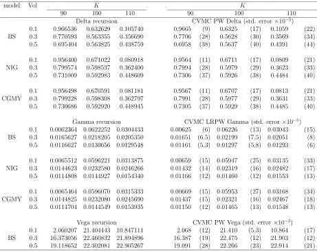
(b) Arithmetic Asian call option price sensitivities.

model Vol K K

90 100 110 90 100 110

Delta recursion CVMC PW Delta (std. error×10−5₎

0.1 0.966536 0.632629 0.105740 0.9665 (9) 0.6325 (17) 0.1059 (22) BS 0.3 0.770593 0.563355 0.356690 0.7706 (28) 0.5628 (30) 0.3569 (34) 0.5 0.695404 0.563825 0.438759 0.6958 (38) 0.5637 (40) 0.4391 (44) 0.1 0.956400 0.671022 0.080918 0.9564 (11) 0.6711 (17) 0.0809 (21) NIG 0.3 0.799574 0.598537 0.362400 0.7994 (28) 0.5979 (29) 0.3623 (33) 0.5 0.731009 0.592983 0.448609 0.7306 (37) 0.5926 (38) 0.4484 (40) 0.1 0.956498 0.670591 0.081181 0.9567 (11) 0.6707 (17) 0.0813 (21) CGMY 0.3 0.799228 0.598308 0.362797 0.7991 (28) 0.5977 (29) 0.3631 (33) 0.5 0.730686 0.592920 0.448945 0.7305 (37) 0.5929 (38) 0.4485 (40)

Gamma recursion CVMC LRPW Gamma (std. error×10−5₎

0.1 0.0062364 0.0622252 0.0304433 0.00625 (6) 0.06226 (13) 0.03043 (15) BS 0.3 0.0165627 0.0218205 0.0205350 0.01651 (6.5) 0.02199 (7.5) 0.02051 (8) 0.5 0.0116627 0.0130656 0.0129548 0.01161 (5.3) 0.01297 (5.8) 0.01293 (6) 0.1 0.0065512 0.0596221 0.0313875 0.00659 (15) 0.05947 (25) 0.03135 (33) NIG 0.3 0.0144623 0.0232580 0.0246266 0.01432 (14) 0.02319 (16) 0.02482 (17) 0.5 0.0114808 0.0144927 0.0154340 0.01166 (12) 0.01460 (12) 0.01553 (13) 0.1 0.0065464 0.0596070 0.0315333 0.00669 (15) 0.05953 (27) 0.03168 (34) CGMY 0.3 0.0144825 0.0232080 0.0245690 0.01437 (15) 0.02321 (16) 0.02467 (18) 0.5 0.0114704 0.0144549 0.0153935 0.01150 (12) 0.01465 (13) 0.01548 (13)

Vega recursion CVMC PW Vega (std. error×10−3₎

0.1 2.060207 21.404443 10.847111 2.068 (12) 21.410 (5.3) 10.864 (17) BS 0.3 16.373056 22.460832 21.894896 16.387 (19) 22.475 (12) 21.903 (12) 0.5 19.118652 22.302081 22.905267 19.091 (28) 22.266 (23) 22.914 (21)

a _{Panel (a) of Table 1 reports the risk neutral model parameters; Panel (b) the arithmetic Asian}

call option price sensitivities. Results are obtained using backward recursions and control variate Monte Carlo (CVMC) simulations with 100,000 trials (standard errors given in parentheses) for the BS, NIG, CGMY models, one-year log-return volatilities Vol =_{0.1,0.3,0.5_} and strike prices

Figure 1

Vega: Asian call vs. plain vanilla call option. Black–Scholes model.

0.1 0.2 0.3 0.4 0.5 0.6 0.7 0.8 0.9 1 5

10 15 20 25 30 35 40

Monitoring dates

Vega

Vol = 10%

0.1 0.2 0.3 0.4 0.5 0.6 0.7 0.8 0.9 1 5

10 15 20 25 30 35 40

Monitoring dates

Vega

Vol = 30%

0.1 0.2 0.3 0.4 0.5 0.6 0.7 0.8 0.9 1 5

10 15 20 25 30 35 40

Monitoring dates

Vega

Vol = 50%

Asian call Vanilla call

a _{Asian call and plain vanilla call option vega comparison in the Black–Scholes model. Vegas}

computed, respectively, using our backward recursion for the Asian option and the closed-form expression for the plain vanilla option. Plain vanilla option maturities coincide with the reset dates of the Asian option. One-year log-return volatilities Vol =_{0.1,0.3,0.5_}. Other parameters:

Figure 2

Convergence patterns of computed deltas, gammas and vegas by backward recursion.

15 16 17 18 19 −4.5

−4 −3.5 −3 −2.5

log₂N

log

10

|Delta

N

− Delta

N/2

|

15 16 17 18 19 −12.5

−12 −11.5 −11 −10.5 −10 −9.5 −9

log₂N

log

10

|Gamma

N

− Gamma

N/2

|

15 16 17 18 19 −8

−7.5 −7 −6.5 −6

log₂N

log

10

|Vega

N

− Vega

N/2

|

NIG CGMY BS

a_{Convergence patterns of numerically computed by backward recursion deltas and gammas (NIG,}

CGMY, BS models) and vegas (BS model) for an at-the-money Asian call option (S0 =K = 100)

and the case of one-year log-return volatility Vol = 0.1 (see Panel (a) of Table 1). DeltaN, GammaN,

Vega_N denote the relevant sensitivities calculated by numerical implementation of the backward recursive integrals (16) and (18) by discrete Fourier transform (see ˇCern´y and Kyriakou, 2011, Section 4) for N discretization points. _|DeltaN −DeltaN/2|, |GammaN −GammaN/2|, |VegaN −

Vega_N/2|are the absolute differences calculated for N = 215_{, . . . ,2}19_{. Other parameters: r = 0.04,}

Figure 3

Convergence patterns of computed vegas and vannas by backward recursion. NIG model.

15 16 17 18 19 −7 −6.5 −6 −5.5 −5 −4.5 −4

Price sensitivity wrt NIG parameter ν

log 2N log 10 |Vega 1, N NIG − Vega 1, N/2 NIG |

15 16 17 18 19 −6 −5.5 −5 −4.5 −4 −3.5

Price sensitivity wrt NIG parameter γ

log 2N log 10 |Vega 2, N NIG − Vega 2, N/2 NIG |

15 16 17 18 19 −4

−3.5 −3 −2.5

Delta sensitivity wrt NIG parameter ν

log 2N log 10 |Vanna 1, N NIG − Vanna 1, N/2 NIG |

15 16 17 18 19 −3.2 −3 −2.8 −2.6 −2.4 −2.2 −2 −1.8

Delta sensitivity wrt NIG parameter γ

log 2N log 10 |Vanna 2, N NIG − Vanna 2, N/2 NIG |

a_{Convergence patterns of computed by backward recursion vegas and vannas with respect to the}

volatility parameters ν and γ of the NIG model for an at-the-money Asian call option (S0 =K =

100) and the case of one-year log-return volatility Vol = 0.1 (see Panel (a) of Table 1). VegaNIG_N , VannaNIG_N denote the relevant sensitivities calculated by numerical implementation of the backward recursive integrals by discrete Fourier transform (see ˇCern´y and Kyriakou, 2011, Section 4) forN