Active Inference: A Process Theory

City, University of London Institutional Repository

Citation

:

Friston, K. J., FitzGerald, T., Rigoli, F., Schwartenbeck, P. & Pezzulo, G. (2017).

Active Inference: A Process Theory. Neural Computation, 29(1), pp. 1-49. doi:

10.1162/NECO_a_00912

This is the published version of the paper.

This version of the publication may differ from the final published

version.

Permanent repository link:

http://openaccess.city.ac.uk/16683/

Link to published version

:

http://dx.doi.org/10.1162/NECO_a_00912

Copyright and reuse:

City Research Online aims to make research

outputs of City, University of London available to a wider audience.

Copyright and Moral Rights remain with the author(s) and/or copyright

holders. URLs from City Research Online may be freely distributed and

linked to.

City Research Online:

http://openaccess.city.ac.uk/

[email protected]

Active Inference: A Process Theory

Karl Friston [email protected]

Wellcome Trust Centre for Neuroimaging, UCL, London WC1N 3BG, U.K.

Thomas FitzGerald [email protected]

Wellcome Trust Centre for Neuroimaging, UCL, London WC1N 3BG, U.K., and Max Planck–UCL Centre for Computational Psychiatry and Ageing Research, London WC1B 5BE, U.K.

Francesco Rigoli [email protected]

Wellcome Trust Centre for Neuroimaging, UCL, London WC1N 3BG, U.K.

Philipp Schwartenbeck

[email protected]

Wellcome Trust Centre for Neuroimaging, UCL, London WC1N 3BG, U.K.; Max Planck–UCL Centre for Computational Psychiatry and Ageing Research, London, WC1B 5BE, U.K.; Centre for Neurocognitive Research, University of Salzburg, 5020 Salzburg, Austria; and Neuroscience Institute,

Christian-Doppler-Klinik, Paracelsus Medical University Salzburg, A-5020 Salzburg, Austria

Giovanni Pezzulo [email protected]

Institute of Cognitive Sciences and Technologies, National Research Council, 00185 Rome, Italy

This article describes a process theory based on active inference and be-lief propagation. Starting from the premise that all neuronal processing (and action selection) can be explained by maximizing Bayesian model evidence—or minimizing variational free energy—we ask whether neu-ronal responses can be described as a gradient descent on variational free energy. Using a standard (Markov decision process) generative model, we derive the neuronal dynamics implicit in this description and reproduce a remarkable range of well-characterized neuronal phenomena. These in-clude repetition suppression, mismatch negativity, violation responses, place-cell activity, phase precession, theta sequences, theta-gamma cou-pling, evidence accumulation, race-to-bound dynamics, and transfer of dopamine responses. Furthermore, the (approximately Bayes’ optimal)

behavior prescribed by these dynamics has a degree of face validity, pro-viding a formal explanation for reward seeking, context learning, and epistemic foraging. Technically, the fact that a gradient descent appears to be a valid description of neuronal activity means that variational free energy is a Lyapunov function for neuronal dynamics, which therefore conform to Hamilton’s principle of least action.

1 Introduction

There has been a paradigm shift in the cognitive neurosciences over the past decade toward the Bayesian brain and predictive coding (Ballard, Hin-ton, & Sejnowski, 1983; Rao & Ballard, 1999; Knill & Pouget, 2004; Yuille & Kersten, 2006; De Bruin & Michael, 2015). At the same time, there has been a resurgence of enactivism; emphasizing the embodied aspect of percep-tion (O’Regan & No¨e, 2001; Friston, Mattout, & Kilner, 2011; Ballard, Kit, Rothkopf, & Sullivan, 2013; Clark, 2013; Seth, 2013; Barrett & Simmons, 2015; Pezzulo, Rigoli, & Friston, 2015). Even in consciousness research and phi-losophy, related ideas are finding traction (Clark, 2013; Hohwy, 2013, 2014). Many of these developments have informed (and have been informed by) a variational principle of least free energy (Friston, Kilner, & Harrison, 2006; Friston, 2012), namely, active (Bayesian) inference.

However, the enthusiasm for Bayesian theories of brain function is ac-companied by an understandable skepticism about their usefulness, par-ticularly in furnishing testable process theories (Bowers & Davis, 2012). Indeed, one could argue that many current normative theories fail to pro-vide detailed and physiologically plausible predictions about the processes that might implement them. And when they do, their connection with a normative or variational principle is often obscure. In this work, we show that process theories can be derived in a relatively straightforward way from variational principles. The level of detail we consider is fairly coarse; however, the explanatory scope of the resulting process theory is remarkable—and provides an integrative (and simplifying) perspective on many phenomena that are studied in systems neuroscience. The aim of this article is to describe the basic ideas and illustrate the emergent processes using simulations of neuronal responses. We anticipate revisiting some is-sues in depth: in particular, a companion paper focuses on learning and the emergence of habits as a natural consequence of observing one’s own behavior (Friston et al., 2016).

policies. This leads to Bayesian belief updates that are informed by beliefs about the future (prediction) and context learning that is informed by beliefs about the past (postdiction). Technically, these updates implement a form of Bayesian smoothing, with explicit representations of states over time, which include future (i.e., counterfactual) states. Furthermore, the implicit variational updates have some biological plausibility in the sense that they eschew neuronally implausible computations. For example, expectations about future states are sigmoid functions of linear mixtures of the pre-ceding and subsequent states. An alternative parameterization, which did not appeal to explicit representations over time, would require recursive matrix multiplication, for which no neuronally plausible implementation has been proposed. Under this belief parameterization, learning is medi-ated by classical associative (synaptic) plasticity. The remaining sections use simulations of foraging in a radial maze to illustrate some key aspects of inference and learning, respectively.

The inference section describes the behavioral and neuronal correlates of belief updating during inference or planning, with an emphasis on elec-trophysiological correlates and the encoding of precision by dopamine. It illustrates a number of phenomena that are ubiquitous in empirical stud-ies. These include repetition suppression (de Gardelle, Waszczuk, Egner, & Summerfield, 2013), violation and omission responses (Bendixen, San-Miguel, & Schroger, 2012), and neuronal responses that are characteris-tic of the hippocampus, namely, place cell activity (Moser, Rowland, & Moser, 2015), theta-gamma coupling, theta sequences and phase precession (Burgess, Barry, & O’Keefe, 2007; Lisman & Redish, 2009). We also touch on dynamics seen in parietal and prefrontal cortex, such as evidence accumula-tion and race-to-bound or threshold (Huk & Shadlen, 2005, Gold & Shadlen, 2007; Hunt et al., 2012; Solway & Botvinick, 2012; de Lafuente, Jazayeri, & Shadlen, 2015; FitzGerald, Moran, Friston, & Dolan, 2015; Latimer, Yates, Meister, Huk, & Pillow, 2015).

The final section considers context learning and illustrates the transfer of dopamine responses to conditioned stimuli, as agents become familiar with experimental contingencies (Fiorillo, Tobler, & Schultz, 2003). We con-clude with a brief demonstration of epistemic foraging. The aim of these simulations is to illustrate how all of the phenomena emerge from a sin-gle imperative (to minimize free energy) and how they contextualize each other.

2 Active Inference and Learning

variational free energy (Friston, 2013). This leads to some surprisingly sim-ple update rules for action, perception, policy selection, learning, and the encoding of uncertainty or its complement, precision. Although some of the intervening formalism looks complicated, what comes out at the end are update rules that will be familiar to many readers (e.g., integrate-and-fire dynamics with sigmoid activation functions and plasticity with asso-ciative and decay terms). This means that the underlying theory can be tied to neuronal processes in a fairly straightforward way. Furthermore, the formalism accommodates a number of established normative approaches, thereby providing an integrative framework.

In principle, the scheme described in this section can be applied to any paradigm or choice behavior. Indeed, earlier versions have been used to model waiting games (Friston et al., 2013), the urn task and evidence accu-mulation (FitzGerald, Schwartenbeck, Moutoussis, Dolan, & Friston, 2015), trust games from behavioral economics (Moutoussis, Trujillo-Barreto, El-Deredy, Dolan, & Friston, 2014; Schwartenbeck, FitzGerald, Mathys, Dolan, Kronbichler et al., 2015), addictive behavior (Schwartenbeck, FitzGerald, Mathys, Dolan, Wurst et al., 2015), two-step maze tasks (Friston, Rigoli et al., 2015), and engineering benchmarks such as the mountain car prob-lem (Friston, Adams, & Montague, 2012). It has also been used in the setting of computational fMRI (Schwartenbeck, FitzGerald, Mathys, Dolan, & Fris-ton, 2015).

In brief, active inference separates the problems of optimizing action and perception by assuming that action fulfills predictions based on in-ferred states of the world. Optimal predictions are therefore based on (sen-sory) evidence that is evaluated using a generative model of (observed) outcomes. This allows one to frame behavior as fulfilling optimistic pre-dictions, where the optimism is prescribed by prior preferences or goals (Friston et al., 2014). In other words, action realizes predictions that are biased toward preferred outcomes. More specifically, the generative model entails beliefs about future states and policies, where policies that lead to preferred outcomes are more likely. This enables action to realize the next (proximal) outcome predicted by the policy that leads to (distal) goals. This behavior emerges when action and inference maximize the evidence or marginal likelihood of the model generating predictions. Note that action is prescribed by predictions of the next outcome and is not itself part of the inference process. This separation of action and perceptual inference or state estimation can be understood by associating action with peripheral reflexes in the motor system that fulfill top-down motor predictions about how we move (Feldman, 2009; Adams, Shipp, & Friston, 2013).

(exploitative) behavior that is formally related to several established ideas (e.g., the infomax principle, Bayesian surprise, the value of information, artificial curiosity, and expected utility theory).

We start by describing the generative model on which predictions and actions are based. We then describe how action is specified by beliefs about states of the world under different policies. The section concludes by con-sidering the optimization of these beliefs through Bayesian belief updating and implicit neuronal processing.

The parameters of categorical distributions over discrete statess∈ {0,1} are denoted by column vectors of expectationss∈[0,1], where the∼ nota-tion denotes sequences of variables over time, for example,s˜=(s₁, . . . ,s_T). The entropy of a probability distributionP(s)=Pr(S=s)is denoted by H(S)=H[P(s)]=E_P[−lnP(s)], while the relative entropy or Kullback-Leibler (KL) divergence is denoted byD[Q(s)||P(s)]=E_Q[lnQ(s)−lnP(s)]. Inner and outer products are indicated byA·B=AT_{B, andA⊗B=AB}T_,

respectively. We use a hat notations=lnsto denote (natural) logarithms. Fi-nally,P(o|s)=Cat(A)implies Pr(o=i|s= j)=Cat(A_{i j}). Definitions of the variables referred to are in Table 1.

Definition. Active inference rests on the tuple(O,P,Q,R,S,T, Υ):

r

r

r

r

r

from (hidden) states s∈S and action u∈Υ

r

and policies π∈T, whereπ∈ {0, . . . ,K} returns a sequence of actions u_t=π(t)

r

0|π). . .Q(sT|π)Q(π)Q(η)over

states, policies and parameters with expectations(sπ₀, . . . ,sπ_T,π,η)

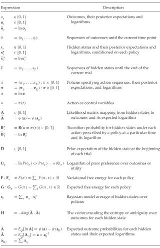
Table 1: Glossary of Expressions.

Expression Description

o_τ ∈ {0,1} Outcomes, their posterior expectations and logarithms

o_τ ∈[0,1]

o_τ =lno_τ

˜

o =(o₁, . . . ,o_t) Sequences of outcomes until the current time point

s_τ ∈ {0,1} Hidden states and their posterior expectations and logarithms, conditioned on each policy

sπ_τ ∈[0,1]

sπ_τ =lnsπ_τ

˜

s =(s₁, . . . ,s_T) Sequences of hidden states until the end of the current trial

π =(π1, . . . , πK):π∈ {0,1} Policies specifying action sequences, their posterior

expectations, and logarithms

π =(π1, . . . ,πK):π∈[0,1]

π =lnπ

u =π(t) Action or control variables

A ∈[0,1] Likelihood matrix mapping from hidden states to outcomes and its expected logarithm

A =ψ(a)−ψ(a₀)

Bπ_τ =B(u=π(τ ))∈[0,1] Transition probability for hidden states under each action prescribed by a policy at a particular time and its logarithm

Bπ_τ =lnBπ_τ

D ∈[0,1] Prior expectation of the hidden state at the beginning of each trial

U_τ =lnP(o_τ)⇔P(o_τ)=σ (U_τ) Logarithm of prior preference over outcomes or utility

F:F_π =F(π )=_τF(π, τ )∈R Variational free energy for each policy

G:G_π=G(π )=_τG(π, τ )∈R Expected free energy for each policy

s_t =_ππ_π·sπ_t Bayesian model average of hidden states over policies

H = −diag(A˘·A) The vector encoding the entropy or ambiguity over outcomes for each hidden state

A =E_Q[lnA]=ψ(a)−ψ(a₀) Expected outcome probabilities for each hidden states and their expected logarithms

˘

2.1 The Generative Model. The generative model is at the heart of (ac-tive) Bayesian inference. In simple terms, the generative model is just a way of formalizing beliefs about the way outcomes are caused. Usually a genera-tive model is specified in terms of the likelihood of each outcome, given their causes and the prior probability of those causes. Inference then corresponds to inverting the model, which means computing the posterior probability of (unknown or hidden) causes, given observed outcomes. In approximate Bayesian inference, this entails optimizing an approximate posterior so that it minimizes variational free energy. In other words, the difficult problem of exact Bayesian inference is converted into an easy optimization prob-lem, where the approximate posterior minimizes a (variational free energy) functional of observed outcomes, under a given generative model. We will see later that when variational free energy is minimized, it approximates the (negative) log evidence or marginal likelihood of the outcomes, namely, the probability of the outcomes under the generative model.

In our case, the generative model can be parameterized in a general way as follows, where the model parameters areη= {a,b,d, β}:

Po˜,s˜, π, η=P(π )P(η)T

t=1P(ot|st)P(st|st−1, π )

Po_t|s_t=Cat(A)

Ps_t+1|s_t, π=Cat(B(u=π(t))) Ps₁|s₀=Cat(D)

P(π )=σ (−γ·G(π )) (2.1)

P(A)=Dir(a) P(B)=Dir(b) P(D)=Dir(d) P(γ )=(1, β).

An approximate posterior over hidden states and parameters x=

(s˜, π, η)can be expressed in terms of its sufficient statistics, which are ex-pectationsx=(sπ₀, . . . ,sπ_T,π,η)andη=(a,b,d,β):

Q(x)=Q(s₁|π ) . . .Q(s_T|π )Q(π )Q(A)Q(B)Q(D)Q(γ )

Qs_t|π=Cat(sπ_t )

Q(π )=Cat(π) (2.2)

Q(D)=Dir(d) Q(γ )=(1,β)

In this model, observations depend only on the current state, while state transitions depend on a policy or sequence of actions. This sequential policy is sampled from a Gibbs distribution or softmax function of expected free energy, with inverse temperature or precision γ. Here G(π ) is the free energy expected under each policy (see below). The role of the model parameters will be unpacked later, when we consider model inversion.

Note that the policy is a random variable that has to be inferred. In other words, the agent entertains competing hypotheses or models of its behavior in terms of policies. This contrasts with standard formulations in which a single state-action policy returns an action as a function of each stateu=π(s), as opposed to time,u=π(t). Furthermore, the approximate posterior is parameterized in terms of expected states under each policy. In other words, we assume that the agent keeps a separate record of expected states—in the past and future—for each allowable policy.

The predictions that guide action are based on a Bayesian model av-erage of these policy-specific states. This means that expectations about policies (and their precision) also have to be optimized. All the posterior probabilities over model parameters, including the initial state, are Dirich-let distributions (FitzGerald, Dolan et al., 2015). The sufficient statistics of these distributions are concentration parameters that can be regarded as the number of occurrences encountered in the past. In what follows, we first describe how actions are selected, given beliefs about the hidden state of the world and the policies currently being pursued. We then turn to the more difficult problem of optimizing the beliefs on which action is based.

2.2 Behavior Action and Reflexes. We associate action with reflexes that minimize the expected difference between the outcomes predicted at the next time step and the outcome following an action. Mathematically, this can be expressed in terms of (outcome) prediction errors as follows:

u_t=min

u EQ[D[P(ot+1|st+1)||R(ot+1|st,u)]]

=min

u ot+1·ε u t+1

εu t+1=

o_t+1−ou_t+1 (2.3)

o_t+1=As_t+1 ou_t+1=AB(u)s_t

s_t=

π

This specification of action is considered reflexive by analogy to mo-tor reflexes that minimize the discrepancy between proprioceptive signals (i.e., primary afferents) and descending motor commands or predictions. Heuristically, action realizes expected outcomes by minimizing the ex-pected outcome prediction error (Adams et al., 2013). Expectations about the next outcome therefore enslave behavior. If we regard competing poli-cies as models of behavior, the predicted outcome is formally equivalent to a Bayesian model average of outcomes, under posterior beliefs about policies (last equality in equation 2.3).

For simplicity, we assume the agent has learned the consequences of ac-tion. More complete schemes would incorporate learning the consequences of action by analogy with learning transitions among hidden states.

Having specified action selection in terms of expected outcomes, we now consider how these expectations are optimized. In active inference, there are no stimulus-response links found in conventional formulations: choices or actions are separated from inference in the same way that peripheral reflexes are separated from processing in the central nervous system. This means all behavior rests on optimizing beliefs or expectations about the next state of the world. These expectations furnish predictions of the next outcome that action simply fulfills. Following action, a new observation becomes available, and the perception-action cycle starts again.

2.3 Free Energy and Expected Free Energy. In active inference, all the heavy lifting is done by minimizing free energy with respect to expectations about hidden states, policies, and parameters. Variational free energy can be expressed as a function of these posterior beliefs in a number of ways:

Q(x)=arg min

Q(x)F

≈P(x|˜o)

F=E_Q[lnQ(x)−lnP(x,o˜)]

=E_Q[lnQ(x)−lnP(x|˜o)−lnP(o˜)]

=E_Q[lnQ(x)−lnP(o˜|x)−lnP(x)] (2.4)

=D[Q(x)||P(x|˜o)]

relative entropy

− lnP(o˜)

log evidence

=D[Q(x)||P(x)]

complexity

−E_Q[lnP(o˜|x)]

accuracy

where o˜=(o₁, . . . ,o_t) denotes observed outcomes up until the current time.

Because KL divergences cannot be less than zero, the penultimate equality in equation 2.4 means that free energy is minimized when the approximate posterior becomes the true posterior. At this point, the free energy becomes the negative log evidence for the generative model (Beal, 2003). This means that minimizing free energy is equivalent to maximizing model evidence, which is equivalent to minimizing the complexity of accu-rate explanations for observed outcomes (the last equality in equation 2.4). With this equivalence in mind, we now turn to the prior beliefs about policies that shape posterior beliefs—and the Bayesian model averaging that determines action. Minimizing free energy with respect to expecta-tions of hidden states and parameters ensures that they encode posterior beliefs, given observed outcomes. However, beliefs about policies rest on outcomes in the future, because these beliefs determine action and action determines subsequent outcomes. This means that policies should, a priori, minimize the free energy of beliefs about the future. Equation 2.1 expresses this formally by making the log probability of a policy proportional to the expected free energy if that policy was pursued. The expected free energy of a policy follows from equation 2.4 (Friston, Rigoli et al., 2015):

G(π )= τ

G(π, τ ),

G(π, τ )=EQ˜[lnQ(sτ|π )−lnP(sτ,oτ|˜o, π )]

=EQ˜[lnQ(sτ|π )−lnP(sτ|oτ,o˜, π )−lnP(oτ)], (2.5)

≈EQ˜[lnQ(sτ|π )−lnQ(sτ|oτ, π )]

(−ve)mutualin f ormation

− EQ˜[lnP(oτ)]

expected log evidence

=EQ˜[lnQ(oτ|π )−lnQ(oτ|sτ, π )]

(−ve)epistemicvalue

−EQ˜[lnP(oτ)]

extrinsicvalue

=D[Q(o_τ|π )||P(o_τ)]

expected cost

+EQ˜[H[P(oτ|sτ)]]

expected ambiguity

,

whereQ˜=Q(o_τ,s_τ|π )=P(o_τ|s_τ)Q(s_τ|π )≈P(o_τ,s_τ|˜o, π )andQ(o_τ|s_τ, π )= P(o_τ|s_τ).

or prior preferences,U(o_τ)=lnP(o_τ), the expected free energy can also be expressed in terms of epistemic and extrinsic value (the penultimate equality in equation 2.5). This means that extrinsic value is the (log) evidence for a generative model expected under a particular policy. In other words, because our model of the world entails prior preferences, any outcomes that provide evidence for our model (and implicit preferences) have pragmatic or extrinsic value. In practice, utilities are defined only to within an additive constant, such that the prior probability of an outcome is a softmax function of utility:P(o_τ)=σ (U(o_τ)). This means prior preferences depend only on utility differences and are inherently context sensitive (Rigoli, Friston, & Dolan, 2016).

Epistemic value is the expected information gain (i.e., mutual

informa-tion) afforded to hidden states by future outcomes and vice-versa.1 _We

will see below that epistemic value can be thought of as driving curiosity and novelty-seeking behavior, by which we resolve uncertainty and ig-norance. A final rearrangement shows that complexity becomes expected cost—namely, the KL divergence between the posterior predictions and prior preferences—while accuracy becomes the accuracy expected under predicted outcomes (i.e., negative ambiguity). This last equality in equa-tion 2.5 shows how expected free energy can be evaluated relatively easily; it is just the divergence between the predicted and preferred outcomes plus the ambiguity (i.e., entropy) expected under predicted states.

In summary, expected free energy is defined in relation to prior beliefs about future outcomes. These define the expected cost or complexity and complete the generative model. It is these priors that lend inference and action a purposeful or goal-directed aspect because they represent prefer-ences or goals. These preferprefer-ences define agents in terms of characteristic states they expect to occupy and, through action, tend to frequent.

There are several interpretations of expected free energy that appeal to and contextualize/established constructs. For example, maximizing epis-temic value is equivalent to maximizing (expected) Bayesian surprise (Schmidhuber, 1991; Itti & Baldi, 2009), where Bayesian surprise is the KL divergence between posterior and prior beliefs. This can also be interpreted in terms of the principle of maximum mutual information or minimum re-dundancy (Barlow, 1961; Linsker, 1990; Olshausen & Field, 1996; Laughlin, 2001). This is because epistemic value is the mutual information between hidden states and observations:I(S_τ,O_τ|π )=H[Q(s_τ|π )]−H[Q(s_τ|o_τ, π )]. In other words, it reports the reduction in uncertainty about hidden states afforded by observations. Because the KL divergence or information gain

1_{Note that the negative mutual information (which is never positive) is not an expected}

cannot be less than zero, it disappears when the (predictive) posterior beliefs are not informed by new observations. Heuristically, this means that epistemic policies will search out observations that resolve uncertainty about the state of the world (e.g., foraging to locate a prey or fixating on informative part of a face, such as the eyes or mouth). However, when there is no posterior uncertainty and the agent is confident about the state of the world, there can be no further information gain, and epistemic value will be the same for all policies, allowing preferences to dictate action.

Conversely, with no preferences (i.e., all outcomes are deemed equally likely), the most likely policies maximize uncertainty over outcomes (i.e., keeping all options open), in accord with the maximum entropy principle (Jaynes, 1957), while minimizing the entropy of outcomes, given the state. Heuristically, this means agents will try to avoid uninformative (low en-tropy) outcomes (e.g., closing one’s eyes) while avoiding states that produce ambiguous (high-entropy) outcomes (e.g., a noisy discotheque) (Schwarten-beck, Fitzgerald, Dolan, & Friston, 2013). This resolution of uncertainty is closely related to satisfying artificial curiosity (Schmidhuber, 1991; Still & Precup, 2012) and speaks to the value of information (Howard, 1966). It is also referred to as intrinsic value (see Barto, Singh, & Chentanez, 2004) for a discussion of intrinsically motivated learning). In one sense, epistemic value can be regarded as the drive for novelty-seeking behavior (Wittmann, Daw, Seymour, & Dolan, 2008; Krebs, Schott, Sch ¨utze, & D ¨uzel, 2009; Schwarten-beck et al., 2013), in which we anticipate uncertainty that can be resolved (e.g., opening a birthday present: see also Barto, Mirolli, & Baldassarre, 2013).

The expected complexity or cost is exactly the same quantity minimized in risk-sensitive or KL control (Klyubin, Polani, & Nehaniv, 2005; van den Broek, Wiegerinck, & Kappen, 2010), and underpins related variational for-mulations of bounded rationality based on complexity costs (Braun, Ortega, Theodorou, & Schaal, 2011; Ortega & Braun, 2013). In other words, minimiz-ing expected complexity renders behavior risk-sensitive, while maximizminimiz-ing expected accuracy induces ambiguity-sensitive behavior. In short, expected free energy covers nearly all measures that have been proposed to explain adaptive behavior, and has each as a special case.

Although the expressions above may appear complicated, expected free energy can be expressed in a simple form in terms of the generative model:

G(π, τ )=D[Q(o_τ|π )||P(o_τ)]

expected cost

+E_Q˜[H[P(o_τ|s_τ)]]

expected ambiguity

=oπ_τ ·(oπ_τ −U_τ)

risk

+sπ_τ ·H

ambiguity

oπ_τ =A˘ ·sπ_τ

oπ_τ =lnoπ_τ

U_τ=U(o_τ)=lnP(o_τ) (2.6)

H= −diag(A˘ ·A),

A=E_Q[lnA]=ψ(a)−ψ(a₀)

˘

A=E_Q[A_{i j}]=a×a−1₀ :a_{0i j}=

i

a_{i j}.

The two terms in the first expression for expected free energy represent risk-and ambiguity-sensitive contributions, respectively, where utility is a vector of preferences over outcomes. This decomposition lends a formal meaning to risk and ambiguity: risk is the relative entropy or uncertainty about outcomes, in relation to preferences, while ambiguity is the uncertainty about outcomes given the state of the world. This is largely consistent with the use of risk and ambiguity in economics (Kahneman & Tversky, 1979; Zak, 2004; Knutson & Bossaerts, 2007; Preuschoff, Quartz, & Bossaerts, 2008), where ambiguity reflects uncertainty about the context (e.g., which lottery is currently in play).

In summary, the above formalism suggests that expected free energy can be carved in two complementary ways. First, it can be decomposed into a mixture of epistemic and extrinsic value, promoting explorative, novelty seeking, and exploitative, reward-seeking behavior, respectively (Friston, Rigoli et al., 2015). Equivalently, minimizing expected free energy can be formulated as minimizing a mixture of expected cost or risk and ambiguity. This completes our description of free energy. We now turn to belief updat-ing that is based on minimizupdat-ing free energy under the generative model we have described.

2.4 Belief Updating and Belief Propagation. Belief updating

medi-ates inference and learning, whereinferencemeans optimizing expectations about hidden states (policies and precision), whilelearningrefers to opti-mizing model parameters. This optimization entails finding the sufficient statistics of posterior beliefs that minimize variational free energy. These solutions are (see appendix A):

sπ_τ =σ (A·o_τ+B_τ−1π sπ_τ−1+Bπ_τ ·sπ_τ+1)

π=σ (−F−γ·G)

β=β+(π−π0)·G

⎫ ⎪ ⎪ ⎬ ⎪ ⎪

A=ψ(a)−ψ(a₀) a=a+_τo_τ⊗s_τ

B=ψ(b)−ψ(b₀) b(u)=b(u)+_{π(τ )=u}π_π·sπ_τ ⊗sπ_τ−1

D=ψ(d)−ψ(d₀) d=d+s₁

⎫ ⎪ ⎪ ⎪ ⎬ ⎪ ⎪ ⎪ ⎭ Learning. (2.7)

For notational simplicity, we have usedBπ_τ =B(π(τ )),D =Bπ₀sπ₀,γ=1/β, andπ₀=σ (−γ·G). Usually one would iterate the equalities in equation 2.7 until convergence. However, we can also obtain the solution in a robust and biologically more plausible fashion using a gradient descent on free energy (see appendixes B and C):

.

sπ_τ =∂

ss

π τ ·επτ

sπ_τ =σ (sπ_τ) .

β=γ2_εγ

επ τ =(

A·o_τ+Bπ_τ−1sπ_τ−1+Bπ_τ ·sπ_τ+1)−sπ_τ εγ_{=(β−β)+(π−π}

0)·G. (2.8)

This converts the discrete updates above into dynamics for inference that minimize state and precision prediction errors επ_τ = −∂_sF and εγ =∂_γF, where these prediction errors are free energy gradients.

Solving these equations produces posterior expectations that minimize free energy to provide Bayesian estimates of hidden variables. This means that expectations change over several timescales: a fast timescale that up-dates posterior beliefs about hidden states after each observation (to min-imize free energy over peristimulus time) and a slower timescale that updates posterior beliefs as new observations are sampled (to mediate evidence accumulation over observations): (see also Penny, Zeidman, & Burgess, 2013). Finally, at the end of each sequence of observations (i.e., trial of observation epochs), the expected (concentration) parameters are updated to mediate learning over trials (FitzGerald, Dolan, & Friston, 2015). These updates are remarkably simple and have intuitive (neurobiological) interpretations:

2.5 Belief Updating and Neuronal Dynamics. Updating hidden states

prior expectations about hidden states with the likelihood of the current observation (Kass & Steffey, 1989). However, the scheme does not use con-ventional forward and backward sweeps (Penny et al., 2013; Pezzulo, Rigoli, & Chersi, 2013), because all future and past states are encoded explicitly. In other words, representations always refer to the same hidden state at the same time in relation to the start of the trial, not in relation to the cur-rent time. This may seem counterintuitive, but this form of spatiotemporal (place and time) encoding finesses belief updating considerably and, as we will see later, has a degree of plausibility in relation to empirical findings.

The formulation in equation 2.8 is important because it describes dy-namics that can be related to neuronal processes. In other words, we move a variational Bayesian scheme toward a process theory that can predict neu-ronal responses during state estimation and action selection (e.g., Solway & Botvinick, 2012). This process theory associates the expected probabil-ity of a state with the probabilprobabil-ity of a neuron (or population) firing and the logarithm of this probability with postsynaptic membrane potential. This fits comfortably with theoretical proposals and empirical work on the accumulation of evidence (Kira, Yang, & Shadlen, 2015) and the neuronal encoding of probabilities (Deneve, 2008), while rendering the softmax func-tion a (sigmoid) activafunc-tion funcfunc-tion that converts membrane potentials to firing rates. The postsynaptic depolarization caused by afferent input can now be interpreted in terms of free energy gradients (i.e., state prediction errors) that are linear mixtures of firing rates in other neurons (or pop-ulations). These prediction errors play the role of postsynaptic currents, which drive changes in membrane potential and subsequent firing rates. This means that when there are no prediction errors, postsynaptic currents disappear and depolarizations (and firing rates) converge to the free energy minimum. Note that the above expressions imply a self-inhibition because prediction errors decrease when log expectations increase.

Technically, replacing the explicit solutions, equation 2.7, with a gradi-ent ascgradi-ent, equation 2.8, is exactly the same generalization of variational Bayes found in variational Laplace (Friston et al., 2007), namely, a gen-eralized coordinate descent. This is nice, because it means one can think about process theories for variational treatments of Markov decision pro-cesses as formally similar to equivalent process theories for state-space models, such as predictive coding (Rao & Ballard, 1999; Bastos et al., 2012). There are some finer, neurobiologically plausible details of the dynamics of expectations about hidden states that we will consider elsewhere. For

ex-ample, the modulation by∂

ss

π

τ implies activity-dependent (e.g., NMDA-R

dependent) depolarization that enforces an excitation-inhibition balance (see appendix B).

the free energy based on past outcomes and the expected free energy based on preferences about future outcomes. In other words, prior beliefs about policies in the generative model are supplemented or informed by the free energy based on outcomes. Policy selection also entails the optimization of expected uncertainty or precision. This is expressed above in terms of the temperature (inverse precision), which encodes posterior beliefs about precision:β=1/γ.

Interestingly, the updates for temperature are determined by the differ-ence between the expected free energy under posterior and prior beliefs about policies, that is, the prediction error based on expected free energy. This endorses the notion of reward prediction errors as an update signal that the brain might use, in the sense that if posterior beliefs based on current observations reduce the expected free energy, relative to prior beliefs, then precision will increase (FitzGerald, Dolan et al., 2015). This can be related to dopamine discharges that have been interpreted in terms of changes in expected reward (Schultz & Dickinson, 2000; Fiorillo et al., 2003) and marginal utility (Stauffer, Lak, & Schultz, 2014). We have previously con-sidered the intimate (monotonic) relationship between expected precision and expected utility in this context (see Friston et al., 2014, for a fuller dis-cussion). The role of the neuromodulator dopamine in encoding precision is also consistent with its multiplicative effect in equation 2.7, to nuance the selection among competing policies (Fiorillo et al., 2003; Frank, Scheres, & Sherman, 2007; Humphries, Wood, & Gurney, 2009; Humphries, Khamassi, & Gurney, 2012; Solway & Botvinick, 2012; Mannella & Baldassarre, 2015). We will return to this later.

2.7 Learning and Associative Plasticity. Finally, the updates for the parameters bear a marked resemblance to classical Hebbian plasticity (Ab-bott & Nelson, 2000). The parameter updates for state transitions comprise two terms: an associative term that is a digamma function of the accumu-lated coincidence of past (postsynaptic) and current (presynaptic) states (or observations under hidden causes) and a decay term that reduces each connection as the total afferent connectivity increases. The associative and decay terms are strictly increasing but saturating functions of the concen-tration parameters. Note that the updates for the connectivity parameters accumulate coincidences over time, because parameters are time invariant (in contrast to states that change over time). Furthermore, the parameters encoding state transitions have associative terms that are modulated by policy expectations.

trial or sequence of observations. This ensures that learning benefits from postdicted states, after ambiguity has been resolved through epistemic be-havior. For example, the agent can learn about the initial state even if the initial cues were completely ambiguous.

Collectively, the updates above constitute a formal description of percep-tion and learning. In what follows, we will associate electrophysiological responses with depolarization (i.e., state prediction error) driving changes in neuronal activity. For simplicity, we recover this from the rate of change of the associated expectation (see equation 2.8).

2.8 Summary. By assuming a generic (Markovian) form for the

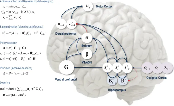
gen-erative model, it is fairly easy to derive Bayesian updates that clarify the relationships among perception, policy selection, precision, and action and how these quantities shape beliefs about hidden states of the world and subsequent behavior. In brief, the agent first infers the hidden states under each model or policy that it entertains. It then evaluates the evidence for each policy based on prior beliefs or preferences about future outcomes. Having optimized the precision or confidence in beliefs about policies, they are used to form a Bayesian model average of the next outcome, which is realized through action. The anatomy of the implicit message passing is not inconsistent with functional anatomy in the brain (see Friston et al., 2014, and Figures 1 and 2). Figure 1 reproduces the (solutions to) belief updating and assigns them to plausible brain structures. Figure 2 rehearses the belief updating in terms of the implicit computations. This functional anatomy rests on reciprocal message passing among expected policies (e.g., in the striatum) and expected precision (e.g., in the substantia nigra). Expecta-tions about policies depend on expected outcomes and states of the world for example, in the prefrontal cortex (Mushiake, Saito, Sakamoto, Itoyama, & Tanji, 2006) and hippocampus (Pezzulo, van der Meer, Lansink, & Pen-nartz, 2014). Crucially, this scheme entails reciprocal interactions between the prefrontal cortex and basal ganglia (Botvinick & An, 2009), in particu-lar, selection of expected motor outcomes by the basal ganglia (Mannella & Baldassarre, 2015).

Figure 1: Schematic overview of belief updates for active inference under dis-crete Markovian models. The left panel lists the solutions in the main text, associating various updates with action, perception, policy selection, precision, and learning. It assigns the variables (sufficient statistics or expectations) that are updated to various brain areas. This attribution should not be taken too se-riously but serves to illustrate a rough functional anatomy, implied by the form of the belief updates. In this simplified scheme, we have assigned observed outcomes to visual representations in the occipital cortex and state estimation to the hippocampal formation. The evaluation of policies, in terms of their (expected) free energy, has been placed in the ventral prefrontal cortex. Ex-pectations about policies per se and the precision of these beliefs have been attributed to striatal and ventral tegmental areas to indicate a putative role for dopamine in encoding precision. Finally, beliefs about policies are used to create Bayesian model averages over future states that are fulfilled by action. The blue arrows denote message passing, and the solid red line indicates a modulatory weighting that implements Bayesian model averaging. The broken red lines indicate the updates for parameters or connectivity (in blue circles) that depend on expectations about hidden states. This scheme is described heuristically in Figure 2. See the appendixes and Table 1 for an explanation of the equations and variables.

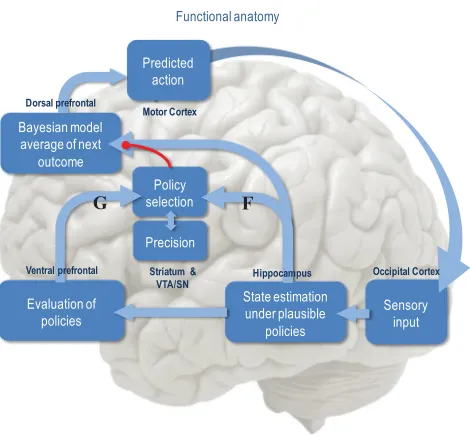
Figure 2: Summary of belief updates in terms of functional anatomy. Sensory evidence is accumulated to optimize expectations about the current state of the world, which are constrained by expectations of past and future states. This corresponds to state estimation under each policy the agent entertains. The quality of each policy is evaluated in the ventral prefrontal cortex, possibly in combination with ventral striatum (van der Meer, Kurth-Nelson, & Redish, 2012), in terms of its expected free energy. This evaluation and the ensuing policy selection rest on expectations about future states. Note that the explicit encoding of future states lends this scheme the ability to plan and explore. After the free energy of each policy has been evaluated, it is used to predict the subsequent hidden state through Bayesian model averaging (over policies). This enables an action to be selected that is most likely to realize the predicted outcome. Once an action has been selected, it generates a new observation, and the cycle begins again.

3 Simulations of Inference

the location of rewards. The basic structure of this problem can be trans-lated to any number of scenarios (e.g., saccadic eye movements to visual targets). The simulations use the same setup as in Friston et al. (2015) and is as simple as possible while illustrating some fairly complicated behav-iors. This example can also be interpreted in terms of responses elicited in reinforcement learning paradigms by unconditioned (US) and conditioned (CS) stimuli. Strictly speaking, our paradigm is instrumental, and the cue is a discriminative stimulus; however, we retain the Pavlovian nomenclature when relating precision updates to dopaminergic discharges.

3.1 The Setup. An agent, such as a rat, starts in the center of a T-maze, where either the right or left arms are baited with a reward (US). The lower arm contains a discriminative cue (CS) that tells the animal whether the reward is in the upper right or left arm. Crucially, the agent can make only two moves. Furthermore, the agent cannot leave the baited arms after they are entered. This means that the optimal behavior is to first go to the lower arm to find where the reward is located and then retrieve the reward at the cued location.

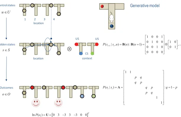
In terms of a Markov decision process, there are four control states that correspond to visiting, or sampling, the four locations (the center and three arms). For simplicity, we assume that each control state takes the agent to the associated location, as opposed to moving in a particular direction from the current location. This is analogous to place-based navigation strategies mediated by the hippocampus (e.g., Moser, Kropff, & Moser, 2008). There are eight hidden states (four locations by two contexts) and seven possible outcomes. The outcomes correspond to being in the center of the maze plus the (two) outcomes at each of the (three) arms that are determined by the context (the right or left arm is more rewarding).

Having specified the state-space, it is now necessary to specify the(A,B) matrices encoding contingencies. These are shown in Figure 3, where the

Amatrix maps from hidden states to outcomes, delivering an ambiguous

cue at the center (first) location and a definitive cue at the lower (fourth)

location. The remaining locations provide a reward with probability p=

98% depending on the context. TheB(u) matrices encode action-specific transitions, with the exception of the baited (second and third) locations, which are absorbing hidden states that the agent cannot leave.

In general treatments, we would consider learning contingencies by up-dating the prior concentration parameters(a,b)of the transition matrices, but we will assume the agent knows (i.e., has very precise beliefs about) the contingencies. This corresponds to making the prior concentration param-eters very large. Conversely, we will use small values ofdto enable context learning. Preferences in the vectorU_τ =lnP(o_τ)≤0 encode the utility of outcomes. Here, the (relative) utilities of a rewarding and unrewarding

out-come were 3 and−3, respectively (and zero otherwise). This means, that

Figure 3: The generative model used to simulate foraging in a three-arm maze (insert on the upper right). This model contains four control states that encode movement to one of four locations (three arms and a central location). These control the transition probabilities among hidden states that have a tensor prod-uct form with two factors: the first is place (one of four locations), and the second is one of two contexts. These correspond to the location of rewarding (red) out-comes and the associated cues (blue or green circles). Each of the eight hidden states generates an observable outcome, where the first two hidden states gen-erate the same outcome that just tells the agent that it is at the center. Some selected transitions are shown as arrows, indicating that control states attract the agent to different locations, where outcomes are sampled. The equations define the generative model in terms of its parameters(A,B), which encode mappings from hidden states to outcomes and state transitions, respectively. The lower vector corresponds to prior preferences—namely, the agent expects to find a reward. Here,⊗denotes a Kronecker tensor product.

a neutral outcome. Note that utility is always relative because the proba-bilities over outcomes must sum to one. As noted above, this means the prior preferences are a softmax function of utilityP(o_τ)=σ (U_τ). Associat-ing utility with log probabilities is important because it endows utility with the same measure as information, namely, nats (i.e., units of information or entropy based on natural logarithms). This highlights the close connection between value and information (Howard, 1966).

each context and zero otherwise. These concentration parameters can be regarded as the number of times each state, transition, or policy has been encountered in previous trials.

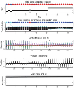
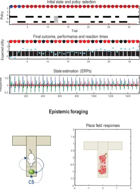
Figure 4 summarizes simulated behavioral and physiological responses over 32 successive trials using a format that will be used in subsequent figures. Each trial comprises two actions following an initial outcome. The first panel shows the initial states on each trial (as colored circles) and sub-sequent policy selection (in image format) over the 10 policies considered. These correspond to staying at the center and then moving to each of the four possible locations (policies 1–4; ending in the center, left, right, or lower arm), moving to the left or right arm and staying there (policies 5 and 6), or moving to the lower arm and then to each of the four locations (policies 7–10). The second panel reports the final outcomes (encoded by colored circles) and performance. Performance is reported in terms of preferred (i.e., utility of) outcomes, summed over time (black bars) and reaction times (cyan dots). Note that because utilities are log probabilities, they are always negative, and the best outcome is zero. The reaction times here are based on the actual processing time in the simulations (using the Matlabtic-toc facility) and are shown after normalization to a mean of zero and standard deviation of one.

In this example, the first couple of trials alternate between the two con-texts with rewards on the right and left. After this, the context (indicated by the cue) remained unchanged. For the first 20 trials, the agent selects epistemic policies—first going to the lower arm and then proceeding to the reward location (i.e., left for policy 8 and right for policy 9). After this, the agent becomes increasingly confident about the context and starts to visit the reward location directly. The differences in performance—between these epistemic and pragmatic behaviors—are revealed in the second panel as a decrease in reaction time and an increase in the average utility. This increase follows because the average is over trials and the agent spends two trials enjoying its preferred outcome when seeking reward directly, as opposed to one trial when behaving epistemically. Note that on trial 12, the agent received an unexpected (null) outcome that induces a degree of posterior uncertainty about which policy it was pursuing, indicated by the red dot. This is seen as a nontrivial posterior probability for three policies: the correct (context-sensitive) epistemic policy and the best alternatives that involve staying in the lower arm or returning to the center. This loss of cer-tainty is accompanied by a low-utility outcome and a suppression of phasic dopamine responses reporting the confidence in behavior.

Neurobiologically, this would entail a selective suspension of belief up-dating, mediated by neuromodulatory projections (omitted from Figure 1). When the agent becomes increasingly confident about the context, the precision of competing policies increases, enabling it to focus on a smaller number and select one quickly and efficiently.

The third panel shows a succession of simulated event-related potentials following each outcome. These are the rates of change of neuronal activity, encoding expectations about hidden states. The fourth panel shows pha-sic fluctuations in posterior precision that can be interpreted in terms of dopamine responses. Here, the phasic component of simulated dopamine responses corresponds to the rate of change of precision (multiplied by eight) and the tonic component to the precision per se (divided by eight; see appendix 5). The phasic part reflects the precision prediction error (cf. reward prediction error: see equation 2.8). These simulated responses re-veal a phasic response to the cue (CS) during epistemic trials that emerges with context learning over repeated trials. This reflects an implicit transfer of dopamine responses from the US to the CS. When the reward (US) is ac-cessed directly, there is a profound increase in the phasic response relative to the response elicited after it has been predicted by the CS.

The final panel illustrates learning in terms of the accumulated posterior expectations about the initial state. The implicit learning reflects an accu-mulation of evidence that the reward will be found in the same location. In other words, initially ambiguous priors over the first two hidden states come to reflect the agent’s experience that it always starts in the first hid-den state. It is this context learning that underlies the pragmatic behavior in later trials. We talk about context learning (as opposed to inference) be-cause, strictly speaking, Bayesian updates to model parameters (between trials) are referred to as learning, while updates to hidden states (within trial) correspond to inference.

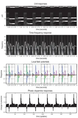
movements in visual exploration (Srihasam, Bullock, & Grossberg, 2009) and the rate at which syllables are articulated in normal speech (Gross et al., 2013). Furthermore, it corresponds to the timescale of neuronal dynamics in the hippocampus (e.g., the duty cycle of theta activity).

Note the changes in activity after each new outcome is observed. For example, the two units encoding the first two hidden states in the first epoch (circled) maintain their firing rate at equivalent levels, reflecting uncertainty about which of the two hidden states are occupied. However, after observing the cue, their activity diverges to properly infer that the first state was the central location under the second context. In other words, representations of the past are informed by current outcomes. The implicit postdiction enables the agent to update its representation (i.e., memory) of the initial state (i.e., past), which it can call on for context learning (see below).

The upper right panel plots the same information, highlighting two units (in solid lines), encoding the upper left and right location on the third epoch. These are the chosen and unchosen states, respectively. Initially, both units encode the same uncertain beliefs about the state that will be occupied, which are resolved in the second epoch and confirmed in the third. The en-suing pattern of firing reflects a saltatory or stepwise evidence accumulation in which expectations about occupying the chosen and unchosen states di-verge as the trial progresses. This belief updating is formally identical to evidence accumulation described by drift diffusion or race-to-bound mod-els (Solway & Botvinick, 2012; Zhang & Maloney, 2012; de Lafuente et al., 2015; Kira et al., 2015) and nicely recapitulates the emergence of a choice as evaluation of options proceeds (Hunt et al., 2012). Furthermore, the separa-tion of timescales implicit in variasepara-tional updating reproduces the stepping dynamics seen in parietal responses during decision making (Latimer et al., 2015).

return to this; however, we first consider the place coding responses of units representing hidden states.

3.3 Theta-Gamma Coupling and Place Cell Activity. The lower right

panel of Figure 5 shows the same firing rate responses above but highlights units encoding the three locations visited (the thick green blue and red lines). These responses reflect increases in activity (during the second theta epoch) in the same sequence that the locations are visited. Empirically, this phenomenon is called a theta sequence: short (3–5) sequences of place cells that fire sequentially within each theta cycle, as if they were encoding time-compressed trajectories (Lisman & Redish, 2009).

In our setting, theta-gamma coupling is a straightforward consequence of belief updating every 250 ms (i.e., theta), where each observation induces phasic updates that necessarily possess high-frequency (i.e., gamma) com-ponents. This is illustrated in the middle left panel of Figure 5, which shows

the response of the second (rewarded hidden state) unit before (dotted line) and after (solid line) filtering at 4 Hz. These responses are superimposed on a time frequency decomposition of the local field potential averaged over all units. The key observation here is that depolarization in the theta range coincides with induced responses, including gamma activity. The implicit theta-gamma coupling during navigation can be seen more clearly in Fig-ure 6. This figFig-ure reports simulated electrophysiological responses over the first eight trials, with the top panel showing the responses of units encoding hidden states and the second panel showing the associated time frequency response (and depolarization of the first unit, after filtering at 4 Hz). The final two panels show the simulated local field potentials and dopamine responses using the same format as the previous figure. The key observa-tion in this here is that fluctuaobserva-tions in gamma power (averaged over all units) are tightly coupled to the depolarization in the theta range (of single units).

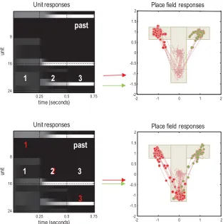
Phase precession and theta-gamma coupling are typically observed in the context of place cell activity, in which units respond selectively when an animal passes through particular locations. This sort of response is easy to demonstrate under the current scheme. Figure 7 (upper right panel) plots the activity of two units encoding the rewarded locations at the right (green dots) and left (red dots) arms as a function of the location in the maze over the first eight trials. The trajectories (dotted lines) were constructed by adding random displacements (with a standard deviation of an eighth) to the trajectory prescribed by action. The dots indicate times at which the unit approached its maximal firing rate (i.e., greater than 80%) and illustrate place cell activity that is specific to the locations they encode. However, this response profile is unique to the units encoding the final location: units encoding the location in the second epoch fire maximally at both the target location and the preceding (cue) location (lower right panel).

Figure 7: Place cell responses. The upper right panel plots the activity of two units encoding the rewarded locations at the right (green dots) and left (red dots) arms, as a function of the location in the maze, over the first eight trials. The trajectories (dotted lines) were constructed by adding (smooth) random displacements (with a standard deviation of an eighth) to the trajectory pre-scribed by action. The dots indicate times at which the unit exceeded 80% of its maximum activity and illustrate place cell activity that is specific to the locations encoded. However, this response profile is unique to the units encoding the final location: units encoding the location in the second epoch fire maximally at both the target location and the preceding (cue) location (lower right panel). The left panel reproduces the neural activity in raster format for two trials to indicate expectations about hidden states that are plotted.

sπ_τ(t+t)=σ (sπ_τ(t)−t·(sπ_τ(t)−. . .−B(π(τ ))·sπ_τ+1(t))),

sπ_τ(t+t)=σ (sπ_τ(t)−t·(sπ_τ(t)−. . .−B(π( t +τ ))·sπ_τ+1(t))). (3.1)

The key difference between these formulations is that in the moving frame of reference, the connectivity changes from epoch to epoch, whereas in a fixed frame of reference, the connectivity remains the same. In light of this, we have elected to simulate responses assuming a fixed frame of reference, which suggests that a subset of hippocampal (or parietal) units should show extraclassical place cell activity, encoding trajectories over multiple locations (Grosmark & Buzsaki, 2016).

4 Context Learning

Having established that the Bayesian updates of expected hidden states and parameters have a degree of biological plausibility, we now turn to the correlates of parameter learning. In this article, the only parameters that are updated are those encoding prior beliefs about the initial state or context. These are the concentration parametersd. In what follows, we look at the effects of context learning on electrophysiological responses and what would happen if we removed prior preferences to reveal purely epistemic behavior.

Figure 8: Repetition suppression and transfer of dopamine responses. This figure uses the same format as Figure 6; however, here we compare two (oddball and standard) trials that are indicated by the arrows on the insert from Figure 4 (upper right). The only difference between these trials is that the agent has become familiar with the context. This means it is more efficient and confident in its inference. This is expressed in terms of a slightly faster and lower-amplitude belief updating about hidden states and increases in expected precision when sampling the cue. The familiarity effects due to repetitions of the standard trials suppress evoked responses in units encoding the first state (cyan circles). This can be seen clearly in the right panel, when we subtract the responses during the standard trial from the equivalent updates during the oddball trial (at the point of anticipation, in the second epoch). The result is a negative difference wave that peaks at around 80 ms (or 180 ms, allowing 400 ms conduction delays). Inspection of the (simulated) phasic dopamine responses shows that the large-amplitude responses to the reward (US) in the first trial are transferred to the cue (CS) after the context has been learned. This pattern corresponds to the transfer of dopamine responses observed in reinforcement learning paradigms.

during learning (Schultz, Apicella, & Ljungberg, 1993; Bromberg-Martin & Hikosaka, 2009). In this instance, the learning corresponds to increasing confidence about the context in which choices are made (Fiorillo et al., 2003). This translates into a higher precision of beliefs about competing policies once the CS has resolved residual uncertainty. Note that this transfer from the US to the CS is direct and does not require any representation of inter-vening states (see (FitzGerald, Dolan et al., 2015) for a fuller discussion). The differences in responses in these two trials can be explained only by differences in prior beliefs about context, because the actions and outcomes were identical. But what about responses when outcomes are unpredicted?

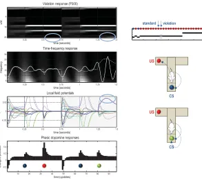
4.2 Violation Responses and Simulated P300 Waveforms. Figure 9

uses the same format as Figure 6 but focuses on consecutive trials after a degree of context learning (the trials indicated by the arrows above the insert from Figure 4). The first trial is a standard one in which the agent interrogates the cue location and then acquires the reward from the appro-priate arm. In the subsequent trial, we forced the agent to stay at the cue location (by preventing it from moving), thereby inducing protracted be-lief updating about hidden states. This is most evident in the hidden state encoding the true location in the third (final) epoch (blue circles). These violation responses reach peak amplitude at about 100 ms—or 200 ms in peristimulus time (allowing for 100 ms conduction delays). Although earlier than classical P300 and N400 responses, this protracted and late response is reminiscent of violation responses in event-related potential (ERP) studies when the outcome is inconsistent with the preceding succession of states, such as semantic violations in sentence processing and action observation (Friederici, 2005; Maffongelli et al., 2015). These late violation responses contrast with the early mismatch responses in the previous figure. Finally, note that the phasic dopamine response to the unexpected outcome is at-tenuated although not abolished. This may reflect the fact that the agent finds it difficult to believe it has not secured its reward. In other words, the agent partly believes it has pursued the epistemic policy despite evidence to the contrary (see upper panel).

4.3 Foraging for Information. One might ask what would happen if

Figure 9: Violation responses and simulated P300 waveforms. This figure uses the same format as the previous figure but focuses on consecutive trials in-dicated by the arrows above the insert. The first trial is an epistemic trial in which the agent interrogates the cue location and then acquires the reward. In the subsequent trial, we forced the agent to stay where it was, thereby induc-ing protracted and high-amplitude belief updatinduc-ing about hidden states. This is most evident in the hidden states encoding the (cue) location in the third (final) epoch (cyan circles). Assuming each epoch lasts 250 ms, these responses reach peak amplitude at about 150 ms—or 250 ms in peristimulus time (allowing for 100 ms conduction delays).

principle, be used to simulate foraging for information using saccadic eye movements.