City, University of London Institutional Repository
Citation:
Brunovsky, P., Černý, A. and Komadel, J. (2018). Optimal Trade Execution Under Endogenous Pressure to Liquidate: Theory and Numerical Solutions. European Journal of Operational Research, 264(3), pp. 1159-1171. doi: 10.1016/j.ejor.2017.07.054This is the accepted version of the paper.
This version of the publication may differ from the final published
version.
Permanent repository link:
http://openaccess.city.ac.uk/17877/Link to published version:
http://dx.doi.org/10.1016/j.ejor.2017.07.054Copyright and reuse: City Research Online aims to make research
outputs of City, University of London available to a wider audience.
Copyright and Moral Rights remain with the author(s) and/or copyright
holders. URLs from City Research Online may be freely distributed and
linked to.
Optimal Trade Execution Under Endogenous Pressure to
Liquidate: Theory and Numerical Solutions
Pavol Brunovsk´ya, Aleˇs ˇCern´yb,∗, J´an Komadela
a
Department of Applied Mathematics and Statistics, Comenius University Bratislava, 84248 Bratislava, Slovakia
b
Cass Business School, City, University of London, 106 Bunhill Row, London EC1Y 8TZ, UK
Abstract
We study optimal liquidation of a trading position (so-called block order or meta-order) in a market with a linear temporary price impact (Kyle, 1985). We endogenize the pressure to liquidate by introducing a downward drift in the unaffected asset price while simultaneously ruling out short sales. In this setting the liquidation time horizon becomes a stopping time determined endogenously, as part of the optimal strategy. We find that theoptimal liquidation strategy is consistent with the
square-root law which states that the average price impact per share is proportional to the
square root of the size of the meta-order (Bershova and Rakhlin, 2013; Farmer et al., 2013; Donier et al., 2015; T´oth et al., 2016).
Mathematically, the Hamilton–Jacobi–Bellman equation of our optimization leads to a severely singular and numerically unstable ordinary differential equation initial value problem. We provide careful analysis of related singular mixed boundary value problems and devise a numerically stable computation strategy by re-introducing time dimension into an otherwise time-homogeneous task.
Keywords: optimal liquidation, price impact, square-root law, singular boundary
value problem, stochastic optimal control
2010 MSC: 34A12, 49J15, 91G80
1. Introduction
We study optimal liquidation of an infinitely divisible asset when the execution price is subject to adverse price impact in proportion to the amount of the asset sold per unit of time, in line with Kyle (1985). The optimal liquidation strategy
∗
Corresponding author
Email addresses: brunovsky@fmph.uniba.sk(Pavol Brunovsk´y),ales.cerny.1@city.ac.uk
trades off expediency against the adverse price impact caused by a precipitous sale. However, our focus on liquidation is not fundamental; mutatis mutandis one can replace optimal liquidation with optimal acquisition in what follows. The novelty in our approach is that we rule out short sales in a falling market. This seemingly small change has a profound impact on the economics and mathematics of the problem. How and why this happens is the subject of the ensuing analysis.
Modelling of optimal execution with market impact is relatively new in the lit-erature, going back to Almgren and Chriss (2000), Bertsimas and Lo (1998) and Subramanian and Jarrow (2001). Classical models Almgren and Chriss (2000), Bert-simas and Lo (1998), envisage a world where the unaffected price of the asset is a martingale and hence there is no pressure to trade quickly for an agent with linear utility. In these circumstances the incentive to trade is given by fiat – it is assumed that there is a fixed time limit by which the entire position must be liquidated.
The literature finds that optimal liquidation gives rise to ‘implementation short-fall’ (Perold, 1988) defined as the gap between the initial market value of the inven-tory and the expected revenue of the liquidation strategy; the latter always being lower due to the price impact. The shortfall itself is formed of two components, one due to ‘permanent price impact’ and another caused by ‘temporary impact’. The former cannot be influenced by the trading strategy, while the latter determines the optimal strategy and can be made arbitrarily small by making the liquidation time horizon longer. In this sense having more time is unambiguously beneficial to the trader.
A second strand of literature, Brown et al. (2010), Chen et al. (2014), Chen et al. (2015), identifies the motive to liquidate with a change in market conditions whereby tighter margin requirements lead to lower permitted amount of leverage. The change in market conditions occurs at discrete time points, while the optimal liquidation (deleveraging) is implemented continuously in time. Here for reasons of tractability the unaffected price is assumed constant during liquidation, although one could in principle use the results from the first strand of literature to make the modelling of the deleveraging phase more realistic.
In this paper we focus on the liquidation phase. Specifically, we study a situation where the unaffected price may be falling on average, which is highly plausible in a market with contracting liquidity. One expects that with the asset price decreasing the implementation shortfall should be more severe than in the martingale case. Surprisingly, the current literature finds that far from exhibiting a shortfall the optimal liquidation strategy may in this case record an expected surplus, see Schied (2013). On closer inspection one observes that the surplus arises due to short sale of the asset with subsequent acquisition at deflated price near the end of the allotted time horizon.
While strategic short sales in a bear market are not entirely implausible we feel it is important to examine a situation where such short sales are ruled out. The
simplest way to achieve this is to stop the trading once the entire position has been liquidated. In doing so we recover the classical outcome from the martingale case whereby the price impact invariably leads to implementation shortfall. However, in a falling market without short sales it is no longer true that the shortfall can be made arbitrarily small by extending the liquidation time horizon.
Introduction of a stopping time is a novel feature in the optimal liquidation lit-erature with a perfectly divisible asset. Previously, optimal stopping has appeared only in the context of optimal liquidation of an indivisible asset, see Mamer (1986) and Henderson and Hobson (2013). Although stopping on liquidation automati-cally precludes short sales, it does leave open the possibility of further intermediate acquisition. Ex-post it turns out that intermediate acquisition is not optimal, see Proposition 7.1 and Theorem 7.2. We show that the presence of the stopping time dramatically changes mathematical properties of the Hamilton-Jacobi-Bellman equa-tion and leads to a severely singular and numerically unstable initial value problem. Part of our research contribution is in providing a comprehensive theoretical and nu-merical analysis of this HJB equation and related singular boundary value problems. The paper is organized as follows. In Section 2 we survey related literature and present our model. In Section 3 we discuss reduction of our HJB partial differential equation (PDE) to an ordinary differential equation (ODE). Section 4 offers a prob-abilistic and control-theoretic interpretation of this reduction. Section 5 describes the singularity of the initial value problem (IVP) for the ODE of Section 3, while Section 6 shows how to obtain uniqueness from a related boundary value problem (BVP). In Section 7 we characterize the optimal strategy and its value function by means of the BVP of Section 6. In Section 8 we introduce and theoretically analyze a related PDE BVP which leads to a stable numerical scheme and present numerical results. Section 9 concludes.
2. Our model and related literature
We take the point of view of a trader with inventoryZwhose initial valueZ(0)> 0 is given. The modelling is based on the premise that there is some price processS– often called the ‘unaffected price’ – with exogenously given dynamics that governs the evolution of the asset price in the absence of our trading. In our case the unaffected priceS is a geometric Brownian motion
dS(t) =λS(t)dt+σS(t)dB(t), (2.1)
whereB is a Brownian motion in its natural filtration.
The inventory attracts interest rate r, which becomes a storage cost when r < 0. We assume that the inventory is sold off continuously at a (stochastic) rate v := −dZ/dt so that v represents the amount of inventory sold per unit of time.
Consequently, the inventory dynamics read
dZ(t) = (rZ(t)−v(t))dt. (2.2)
Let T(Z = 0) be the first time when the entire inventory is disposed of. For a given pair of initial values
s=S(0), z=Z(0), (2.3)
the expected discounted revenue from the disposal of the asset is given by
J(s, z, v) =Es,z "
Z T(Z=0)
0
e−ρt(S(t)−ηv(t))v(t)dt
#
, (2.4)
whereS−ηvis the ‘affected price’ of the asset. In our settingηmeasures the strength of ‘temporary impact’ the selling speed v has on the price. The discount factor ρ captures the opportunity cost of not holding alternative assets. The entire model is based on ˇCern´y (1999).
The task is to find optimal liquidation strategy v that maximizes
V(s, z) := sup
v∈A
J(s, z, v). (2.5)
We say that v is an admissible control, and writev ∈ A, if processv is predictable,
E
Z t
0
|v(s)|mds
<∞for all t >0 andm= 1,2, . . . , (2.6)
and
E
Z T(Z=0)
0
e−ρs|v(t)(S(t)−ηv(t))|dt
!
<∞. (2.7)
The optimization in our model can be seen, for specific parameter choices, as a special case of Ankirchner and Kruse (2013), Forsyth et al. (2012) and Schied (2013), with the crucial difference that in our case the liquidation time horizon is endogenous. We make a standing assumption that the time discounting is stronger than the expected appreciation and the interest on the asset combined,
ρ > λ+r. (2.8)
To conclude this section we wish to make several observations that justify the choice of our modelling framework. The extant literature contains a number of variations on the model presented above. The trading may be discrete, rather than continuous, the unaffected priceS may be specified differently and the optimization criterion may involve a utility function. In common, existing models assume T is fixed and exogenously given.
The most commonly considered specification for the affected price reads
˜
S :=S−γ(Z(0)−Z−−1
2∆Z)−η1v+η2∆Z, (2.9) where γ(Z(0)−Z−−1
2∆Z) is the ‘permanent’ price impact
1 while η
1v and η2∆Z,
respectively, are known as ‘temporary’ price impacts in the continuous-time and discrete-time literature, respectively. It is assumed either that there is a finite number of fixed dates{ti}Ni=1 where Z is allowed to jump (discrete-time models) or that Z
changes continuously at a stochastic time rate−v(continuous-time models). In each case Z is taken to be a predictable semimartingale with left limit process Z− and jumps ∆Z = Z −Z−. Models in this category include Ankirchner et al. (2016), Brown et al. (2010), Chen et al. (2014), Gatheral and Schied (2011), Schied (2013), Schied and Sch¨oneborn (2009) Ting et al. (2007) in continuous time and Almgren and Chriss (2000), Bertsimas and Lo (1998) in discrete time. Other impact specifications can be found, for example, in Chen et al. (2015), Cheridito and Sepin (2014), Forsyth (2011), Lorenz and Almgren (2011), Subramanian and Jarrow (2001) and Ting et al. (2007).
The revenue R(T) from liquidation over a fixed time horizon T is given by R(T) := RT
0 −S(t)dZ(t). When the unaffected asset price process˜ S is a
martin-gale, integration by parts together with suitable boundedness of Z and boundary condition Z(T) = 0 yields
E[R(T)] =Z(0)S(0)−γ
2Z(0)
2−η 1
Z T
0
v2(t)dt−η2
N X
i=1
(∆Z(ti))2.
This equality offers several important insights:
1. Permanent impact (as defined here) has no strategic influence and in the ab-sence of temporary impact (η1 = η2 = 0) any strategy Z is optimal. The expected implementation shortfall Z(0)S(0)−E[R(T)] = γ2Z(0)2 is strictly
positive.
2. With temporary impact it is optimal to liquidate at a constant rate, regard-less of the strength of the permanent impact. The additional implementation shortfall equalsη1Z(0)2/T in continuous time andη
2Z(0)2/N in discrete time,
respectively.
These observations suggest that temporary impact is responsible for the major-ity of strategic interaction also in the drifting market and we conjecture that the
1Note that this classification of permanent impact differs subtly from the one used in Almgren
and Chriss (2000) and subsequent literature. In our classification permanent impact has no strategic effect on optimal execution whenS is a martingale.
optimalstrategy will therefore not change dramatically when the permanent impact is included. This is not to say that the implementationshortfall would be unaffected by the presence of permanent impact. Given the complexity of analysis to follow and the likely marginal gains to our understanding from the presence of permanent impact on the optimal trading strategy we feel justified in leaving out the permanent impact from our analysis.
More recent studies, excellently summarized in Gatheral (2010), consider an in-termediate form of impact where the execution price is given by the formula
St− Z t
0
f(vu)G(t−u)du.
KernelGis called theresiliency of the market and the two extreme cases, permanent impact and temporary impact, correspond toGbeing constant orGbeing the Dirac delta function, respectively. In Gatheral (2010) a case is made for a combination of power impact function,f(v) =vδ, with power law resiliencyG(x) =x−γ,δ+γ ≥1, the latter tending to a Dirac delta function as γ & 0. We note that our setup corresponds to the limiting caseδ= 1, γ= 0 and we leave the analysis of the general impact function f with general resiliency G in the setup of this paper to future research.
3. HJB equation and dimension reduction
The value functionV defined in (2.5) formally solves the Hamilton-Jacobi-Bellman partial differential equation
sup
v
{1
2s
2σ2V
ss+λsVs+ (rz−v)Vz−ρV +v(s−ηv)}= 0, s >0, z >0,
with formal optimal control
v∗ = s−Vz 2η ,
giving rise to a quasilinear second order PDE
1 2s
2σ2V
ss+λsVs+rzVz−ρV +
(s−Vz)2
4η = 0, (3.1)
with an initial condition
V(s,0) = 0. (3.2)
The self-similarity
reduces (3.1, 3.2) to an initial value problem (IVP) for an ordinary differential equa-tion (ODE)
x2u00=axu0+bu−(u0−1)2/2, x >0, (3.4)
u(0) = 0, (3.5)
where
a:= 2(λ−r+σ2)/σ2, b:=−2(2λ−ρ+σ2)/σ2. (3.6) The self-similarity reduces a problem with 7 independent parametersρ, λ, r, σ, η, s≡
S(0) andz≡Z(0) to a problem with just three parameters: a, band x:=ησ2z/s.
4. Probabilistic interpretation of self-similarity
We begin by restating the HJB equation (3.1) in its variational form,
sup
v(0)
drift0 e−ρtV(S, Z)
+v(0) (S(0)−ηv(0)) = 0.
Plug in the self-similarity form of the value functionV(S, Z) =S2u ησ2Z/S/(ησ2) and rearrange to obtain
sup
v(0)
drift0
e−ρt S
2
S(0)2u
ησ2Z S
+ησ2v(0) S(0)
1−ηv(0) S(0)
= 0.
The next steps involve i) changing measure to ˆP given by dPˆt
dPt =
S(t)2 S(0)2e
−(2λ+σ2)t
where ˆPt and Pt are restrictions of ˆP and P toFt; ii) defining a new state variable
X:=ησ2Z/S; and iii) reparametrizing the control to g:=ηv/S,which yields sup
g(0)
n
d
drift0
e(2λ+σ2−ρ)tu(X)
+σ2g(0) (1−g(0))
o
= 0. (4.1)
The It¯o formula for X reads
dX = rX−σ2g
dt+X
−dS
S +
d[S, S] S2
,
while from the Girsanov theorem we obtaindrift (d L(S)) =λ+ 2σ2, which implies
dX = (r−λ−σ2)X−σ2g
dt+σXdB,ˆ (4.2)
where ˆB :=−L(S)/σ+(λ+2σ2)t/σis a Brownian motion under ˆP andL(S) denotes
the stochastic logarithm of S, dL(S) = dS/S. In the final step we perform a time
change fromt toσ2t, defining ˆX(t) :=X(t/σ2) and ˆW(t) :=σB(t/σˆ 2). This yields the dynamics
dXˆ =
r−λ−σ2 σ2 Xˆ −g
dt+ ˆXdW ,ˆ (4.3)
while (4.1) changes to
sup g(0) d drift0 exp
2λ+σ2−ρ σ2 t
u( ˆX)
+g(0) (1−g(0))
= 0. (4.4)
With (4.3) in hand the optimality condition (4.4) explicitly reads
0 = 1 2x
2u00(x) +r−λ−σ2 σ2 xu
0(x)
+2λ+σ
2−ρ
σ2 u(x) +
1 4 1−u
0(x)2
,
and the (formal) optimal control equals g = (1−u0( ˆX))/2. It is furthermore clear that (4.4) itself is a HJB equation of an optimal control problem
u(x) = sup
g b
Ex= ˆX(0)
"
Z T( ˆX=0)
0
exp
−ρ−2λ−σ
2
σ2 t
g(t)(1−g(t))dt
#
, (4.5)
with ˆP-dynamics of ˆX given by (4.3).
Note that the time in the transformed problem (4.5) is measured in terms of cumulative variance of the log return of the unaffected price, that is in ‘variance years’. One variance year corresponds to the physical timetit takes to makeσ2t= 1. With σ = 0.2 one variance year is therefore equal to 25 calendar years. The new state variable ˆX = ησ2Z/S corresponds to the size of temporary price impact as a percentage of current price, assuming inventory Z is completely liquidated at a constant rate over one variance year.
5. Singular initial value problem IVP0
Hereafter we refer to the IVP (3.4, 3.5) as IVP0. Notea+b >0 if and only if our
standing assumption (2.8) ρ > r+λholds. It has been shown in Brunovsk´y et al. (2013) that IVP0 is highly degenerate at 0.For a+b >0 IVP0 has infinitely many
solutions with identical asymptotics near 0 given by the formal power series
hn(x) =x−
2 3
p
2(a+b)x3/2+
n X
i=2
kix1+i/2, n∈N, (5.1)
whereki are obtained recursively from
kn+1 =
1 3 (n+ 3)k1
kn((n+ 2) (2a−n) + 4b)
−1
2
n−1
X
j=1
(3 +j)(n−j+ 3)kj+1kn−j+1
.
The series itself has zero radius of convergence for
6a+ 4b−3 =:K1 >0> K2 := 6a+ 2b−9,
see (Quittner, 2015, Remark 2). Asymptotic expansion of derivatives of u(x) is obtained by formal differentiation of the series in (5.1), ibid Theorem 1. Whenever K1= 0 orK2 = 0 the power series ends at the 3rd element and constitutes a genuine
solution of IVP0. This solution, however, is just one from a continuum and does not
represent the optimal value function.
The highly degenerate nature of IVP0 does not stem from the singularity of the
linear terms in the ODE, which is well known and rather innocuous in the context of the Black-Scholes model, but from the singularity of the non-linear term. Liang (2009) studies singular IVPs of the form u00 =x−1f(x, u, u0) wheref is continuous. Note that the linear part of our ODE,ax−1u0,belongs to Liang’s category, but the non-linear termx−2(u0−1)2/2 does not.
Liang, too, observes multiplicity of solutions, but this multiplicity is less pro-nounced than in our case. In Liang’s work u(0) and u0(0) uniquely determine the firstdγederivatives of the solution, whereγ := ∂u∂0f(0, u(0), u0(0))>0, and, for
non-integerγ, the solution becomes unique once the coefficient byxγ has been specified. Therefore, in Liang’s case all solutions differ asymptotically by a multiple ofxγ near 0.
In contrast, IVP0 has a continuum of solutions that differ asymptotically by
xαexp −β/√x, where
α:= 2−2
3b, β:=
p
8(a+b),
see (Quittner, 2015, Theorems 2-5). These solutions invariably share their power series asymptotics to an arbitrary order as x &0. A uniqueness result relevant for the current paper can be summarized as follows:
Proposition 5.1. Under the assumption a+b > 0 there is a unique solution of
IVP0 denoted by u∞ satisfying u∞∈ C0([0,∞))∩ C2((0,∞)),
0≤u∞(x)≤x for x >0. (5.2)
The solution u∞ further satisfies u0∞(0) = 1, u0∞(x) >0, u00∞(x) < 0, u000∞(x)> 0 for
Proof. See Proposition 5.1 in Brunovsk´y et al. (2013).
Proposition 5.2 reveals certain qualitative characteristics of solutions of IVP0
which can be observed empirically whenever an unstable numerical scheme is em-ployed.
Proposition 5.2. Any solution of (3.4) on (α, β) with 0 ≤ α < β ≤ ∞ falls into one and only one of the following categories:
i) u is constant;
ii) u is strictly concave on (α, β);
iii) u is strictly convex on (α, β);
iv) there is x0 ∈(α, β) such that u is strictly concave on (α, x0), strictly convex
on(x0, β) andu0(x)≥u0(x0)>0 for allx∈(α, β);
v) there is x0 ∈ (α, β) such that u is strictly convex on (α, x0), strictly concave
on(x0, β) andu0(x)≤u0(x0)<0 for allx∈(α, β).
Proof. The conclusions follow readily from Brunovsk´y et al. (2013), Lemma 4.1,
applied to the equation
x2y00= (1 + (a−2)x−y))y0+ (a+b)y, (5.3) withy=u0, obtained by differentiation and re-arrangement of (3.4).
6. Boundary value problem BVP[0,∞)
In the context of the present paper it turns out to be advantageous to view Proposition 5.1 as a solution to a certain boundary value problem (BVP). We write u0(∞) := limx→∞u0(x) whenever the limit on the right-hand side exists and comple-ment the Dirichlet-type boundary conditionu(0) = 0 with a Neumann-type bound-ary condition
u0(∞) = 0. (6.1)
Hereafter we refer to the mixed boundary value problem (3.4, 3.5, 6.1) as BVP[0,∞).
It is seen below that the right-hand boundary condition (6.1) uniquely determines the solution found in Proposition 5.1.
Proposition 6.1. Under the assumption a+b >0 BVP[0,∞) has a unique solution
which additionally satisfiesu0(0) = 1,u0>0,u00<0, u000>0, as well as0≤u(x)≤
x.
Proof. BVP[0,∞) possesses at least one solution, namely the solution identified in
Proposition 5.1. Below we will prove uniqueness by showing that any solution of BVP[0,∞) must also satisfy 0≤u(x)≤x. By Lemma 3.1 in Brunovsk´y et al. (2013)
any local solution of the IVP0 satisfies limx→0+u
0(x) = u0(0) = 1. Consider now
the alternatives in Proposition 5.2 with α = 0 and β = ∞. Since any solution of BVP[0,∞) also solves IVP0 it cannot fall into the constant alternative i). Similarly,
it cannot fall into category iii) withu00>0 sinceu0(0) = 1 then implies u0(∞)≥1. Alternatives iv) and v) also implyu0(∞)6= 0. Therefore only category ii) remains as a possible alternative. One thus obtains u00 < 0 globally, therefore u0 is decreasing and u0(∞) = 0 implies u0 ≥ 0.We have thus proved 0 ≤u0 ≤1 and on integrating one obtains 0≤u≤x. This shows uniqueness by Proposition 5.1.
The paper Brunovsk´y et al. (2013) left two questions open. The first is whether the value function V generated by the solution u∞ of BVP[0,∞) from Proposition
5.1 via equation (3.3) is indeed the value function of the optimization problem (2.5). The second question concerns numerical computation of the solution to BVP[0,∞).
We address both questions in turn, the former in Section 7 and the latter in Section 8.
7. Optimality
In this section we establish the precise connection between the boundary value problem BVP[0,∞) and the optimal control and value function for the liquidation
problem (2.5). We begin by formulating a natural sufficient condition for admissi-bility and investigate under what circumstances it is admissible to pursue further acquisition of the asset to be liquidated,v <0.
Proposition 7.1. Under the assumption (2.8) any predictable control v satisfying
S(t)/η ≥v(t)≥0 is admissible. If additionally
ρ > λ++r+, (7.1)
wherex+ := max(x,0),then any predictable controlv satisfyingS(t)/η ≥v(t)≥ −K
for some K >0 is also admissible.
Proof. i) We have |v(t)|m ≤ (S(t)/η)m +Km and since S is a GBM this implies
EhRt
0|v(s)|
mdsi<∞ for any finitet and anym∈
Nwhich proves (2.6).
ii) To prove (2.7) first note that v(t)≥ −K implies
Z(t)≤zert+Ke
rt−1
r . (7.2)
To show integrability of the value function we first obtain an estimate of the integrand
|v(t)(S(t)−ηv(t))| ≤ v(t)++v(t)−
S(t) +ηv(t)−
≤ K+v(t)+
(S(t) +ηK),
which for any bounded stopping timeτ yields
E
Z τ
0
e−ρt|v(t)(S(t)−ηv(t))|dt
≤K
Z τ
0
e−ρt(E[S(t)] +ηK)dt+E
Z τ
0
e−ρtv(t)+(S(t) +ηK)dt
≤K
Z ∞
0
e−ρt(seλt+ηK)dt
| {z }
C<∞
+E
Z τ
0
e−ρtv(t)+(S(t) +ηK)dt
.
Continue with the integral inside the expectation in the second term, lettingW(t) =
Rt
0v(s)
+ds, and integrating by parts. In preparation note dZ(t) = (rZ(t)−v(t))dt
which together with (7.2) implies for any bounded stopping time τ ≤T
0 ≤ W(τ) =
Z τ
0
v(t)+dt=
Z τ
0
v(t)−dt+
Z τ
0
rZ(t)dt+z−Z(τ)
≤ Kτ+
Z τ
0
r
zert+Ke
rt−1
r
dt+z=:g(τ). (7.3)
Integration by parts yields
Z τ
0
e−ρtv(t)+(S(t) +ηK)dt = e−ρτW(τ) (S(τ) +ηK) +ρ
Z τ
0
e−ρtW(t) (S(t) +ηK)dt−
Z τ
0
e−ρtW(t)dS(t).
We continue with the second term on the right-hand side. LetdM(t) =e−ρtW(t)S(t)dB(t)
then E[[M, M]t] = E h
Rt
0e
−2ρlW2(l)S2(l)dli ≤s2Rt
0 g
2(l)e2(λ+σ2−ρ)l
dt < ∞ with g from (7.3) which implies thatM is a (square-integrable) martingale. Hence for any bounded stopping timeτ
E
Z τ
0
e−ρtW(t)dS(t)
=E
Z τ
0
e−ρtλW(t)S(t)dt
.
Pulling everything together
E
Z τ
0
e−ρt|v(t)(S(t)−ηv(t))|dt
≤C+E
Z τ
0
e−ρtv(t)+(S(t) +ηK)dt
.
The right-hand side is bounded for K = 0 under the standing assumption (2.8). This is also true for K > 0 if additionally ρ > 0, ρ > λ and ρ > r. The last three inequalities together with the standing assumption (2.8) are equivalent to (7.1). Lettingτ increase to T we have by monotone convergence
E
Z T
0
e−ρt|v(t)(S(t)−ηv(t))|dt
<∞.
The next theorem characterizes the optimal liquidation strategy and the corre-sponding value function. The inequality V(s, z) ≤ sz confirms the initial intuition that without short sales the implementation shortfallsz−V(s, z) must be positive. We note that due to 0≤u0∞(x)≤1 we havev∗(t)≥0,i.e. it isnot optimal to buy more of the liquidated asset, even when (for ρ > λ++r+) strategies that involve further purchases are admissible.
Theorem 7.2. Assume (2.8). Let u∞ be the unique solution of BVP[0,∞), with
a, b given by (3.6). Then the function V(s, z) := ησs22u∞ ησ2zs
≤ sz is the value
function of the optimization (2.5) and
v∗(t) := 1
2η(S(t)−Vz(S(t), Z
∗(t))) = S(t) 2η
1−u0∞
ησ2Z ∗(t)
S(t)
≥0 (7.4)
is the optimal control among all admissible controlsA defined in equations (2.6,2.7).
Proof. To prove the theorem we apply the ‘Verification’ Theorem IV.5.1 of Fleming
and Soner (2006). To this end, we have to check the following:
(i) V(s, z) isC2((0,∞)×(0,∞))∩ C0([0,∞)×[0,∞)) and satisfies
|V(s, z)| ≤K(1 +|(s, z)|m)
for somem >0, K >0; (ii) lim supt→∞E(s,z)
It≤T(Z=0)e−ρtV(S(t), Z(t))
≥ 0 for all admissible controls, wheres:=S(0) andz:=Z(0);
(iii) For deterministict
lim
t→∞e −ρtE
(s,z)
It≤T(Z∗=0)V(S(t), Z∗(t))= 0,
(S(t), Z∗(t)) being the solution of
dS(t) =λS(t)dt+σS(t)dB(t),
dZ∗(t) =
rZ∗(t)−S(t)
2η
1−u0
ησ2Z ∗(t)
S(t)
dt.
The regularity properties as well as the estimates of (i) and (ii) are immediate consequences of the properties ofu∞, which in particular imply
0≤V(s, z)≤sz. (7.5)
The estimate (7.2) givesZ∗(t)≤zertwhich in combination with inequality (7.5) and standing assumption (2.8) yields
0 ≤ e−ρtE(s,z)
It≤T(Z∗=0)V(S(t), Z∗(t))
≤ e−ρtzertE(s,z)[S(t)] =sze(r+λ−ρ)t&0. This proves item (iii).
Observe that the optimal control deviates from the myopic strategy of maximizing the integrand of the objective function vmyopic(t) := S(t)/(2η). In addition to the
instantaneous impact on the execution price the current liquidation rate also affects future levels of the inventory Z. In (7.4) the optimal strategy at time t differs from vmyopic(t) by the amount −Vz(S(t), Z∗(t)), which is the marginal value of the
optimal revenue with respect to the size of the remaining inventory. It follows that taking proper account of the role of future inventory level reduces the selling rate. By Proposition 5.1, u0∞ is positive and decreasing to zero and so is Vz(s, z) in z
and therefore for large values of Z∗(t) the selling rate is very close to the myopic strategy. For small values ofZ∗(t) the optimal rate of trading is non-linear, roughly proportional to √Z as can be seen from the asymptotic expansion (5.1) and the formula for the optimal trading rate (7.4).
We remark that the classical martingale case with ρ=λ=r = 0 and fixed time horizon T yields constant optimal liquidation speed v∗ = Z(0)/T. The resulting price impact per share, for fixed T, is proportional to Z(0) which is not consistent with broad empirical evidence that indicates power dependence roughly proportional topZ(0).
When estimating price impact empirically, an assumption has to be made about the rate of trading. In Almgren et al. (2005) this rate is assumed to be constant and the temporary impact of individual trades is estimated proportional to v0.6 which yields per-share temporary price impact proportional to Z(0)0.6. Here, in contrast, the temporary impact is linear, proportional tov, but the optimal rate of trading is non-linear, roughly proportional to√Z for small values. ‘Small’ must be understood in context; we find that √Z asymptotics is perfectly compatible with meta-orders whose optimal execution lasts several days, see Section 8.4.
We can also make qualitative conclusions about the optimized implementation shortfall by studying the asymptoptic expansion (5.1) whereby we find that for small Z(0) the per-share price impact equals
I(S(0), Z(0)) = S(0)Z(0)−V(S(0), Z(0))
S(0)Z(0) =
4 3
p
η(ρ−λ−r)Z(0)/S(0)+O(Z(0)3/2), which means that the price impact is proportional to the square root of the total trade size. There is a strong empirical evidence to support the square root law for meta-orders, see Bershova and Rakhlin (2013), Farmer et al. (2013), Donier et al. (2015) and T´oth et al. (2016) and references therein.
8. Computation of the solution
To make BVP[0,∞) amenable to numerical treatment we first truncate the spatial
interval to x ∈ [ε, L] with ε ≥ 0, L < ∞ and solve the ODE (3.4) with mixed boundary conditions u(ε) = 0 and u0(L) = 0. We refer to the truncated boundary
value problem as BVP[ε,L]. In section 8.1 we prove that the solutionuL of BVP[0,L]
is unique and that it converges pointwise upwards to the desired solution u∞ as L% ∞.
Numerical solutions of BVPs for ordinary differential equations with singular co-efficients have a well established literature, see for example Jamet (1969), Weinm¨uller (1984), Weinm¨uller (1986), and Auzinger et al. (1999) who consider BVPs with ODE of the form
u00=x−1A(x)u0+x−2B(x)u+F(x, u, u0), (8.1) where A, B and F are continuous at x = 0 and one of the boundaries is x = 0. Numerical solution of (8.1) can be computed by means of the Matlab functionbvp5c
after transformationy(x) = [u(x) xu0(x)], see Weinm¨uller (1986), equation (2.1a). However, as we have mentioned already in the connection with IVP0, our problem
BVP[0,L]is substantially more singular. This is not due to the singularity in the linear terms of ODE (3.4), which in fact can be accommodated in the ansatz (8.1), but because the non-linear part F(x, u, u0) = 12x−2(u0 −1)2 is not continuous in x at zero. Attempts to compute the solution of BVP[0,L] by some kind of shooting fail – both at x → 0 and x → ∞ the trajectories blow up. Algorithm bvp5c is able to produce, with careful tuning of input parameters, a stable solution of BVP[ε,L]forε
not too close to zero. However, the quality of this solution near zero is poor, as can be seen in panel (b) of Figure 1.
To bypass the troublesome singularity at zero we introduce a time dimension into BVP[0,L] in a strategy akin to thevalue function iteration method known from
financial economics. This approach is also common in linear-quadratic optimal con-trol problems where, however, it is not motivated by the presence of singularities, see Anderson and Moore (1989, Section 3.1).
We consider a parabolic PDE that corresponds to a finite horizon version of the time-homogeneous optimization (2.5). We formulate suitable boundary conditions on a finite spatial intervalx∈[0, L] to obtain a parabolic problem BVPt[0,L]and show that its solution converges monotonically to the solution of BVP[0,L]ast→ ∞. This is done in section 8.2. Unfortunately, BVPt[0,L] does not correspond to an optimal control problem due to the choice of boundary conditions.
In section 8.3 we formulate a finite difference scheme to solve BVPt[0,L] numer-ically. This scheme is well behaved with respect to the singularity at x = 0 and produces a reliable approximation to uL, which for large enough L is arbitrarily
close to the desired solution u∞.
8.1. Problem BVP[0,L]
Theorem 8.1. Let a+b >0. For given L >0 BVP[0,L] has a unique solutionuL∈
C2((0, L])∩C0([0, L]) such that0≤uL(x)≤x for allx∈[0, L]. The solutionuL is
strictly increasing, concave and satisfies uL1(x)≤uL2(x) for L1 ≤L2, 0≤x≤L1,
and limL→∞uL(x) = u∞(x) for 0 ≤ x < ∞, where u∞ is the unique solution of
BVP[0,∞).
Proof. Step 1)For anyε >0 such thatε < Lthe functionα(x) := 0, resp. β(x) :=x
is a lower (resp. upper) solution of BVP[ε,L] in the sense of Definition II.1.1 in
De Coster and Habets (2006), which crucially allows for the Neumann boundary condition at L. Therefore by Theorem II.1.3 ibid the solution uε of the mixed
boundary value problem BVP[ε,L] satisfies
0≤uε(x)≤x for everyε >0. (8.2)
From here the proof proceeds as in Proposition 2.2 of Brunovsk´y et al. (2013). From Bernstein’s condition Bernstein (1904) (see also Section I.4.3 of De Coster and Habets (2006) for related Nagumo condition) fixing ˜ε > 0 we obtain a uniform (in ε) a-priori bound on the derivative u0ε on [˜ε, L]. Together with (8.2) this yields via (3.4) an a-priori bound on u00ε on [˜ε, L] which means {u0ε}ε>0 (as well as {uε}ε>0) are
equicontinuous on [˜ε, L] which in turn implies equicontinuity of {u00ε}ε>0 via (3.4). One can thus extract a convergent subsequence of u1/k which convergences with its first two derivatives to some function u on (0, L] with u(0) = 0 and such that u solves (3.4).
Step 2) By Brunovsk´y et al. (2013), Lemma 3.1,u0L(0) = 1. This, together with
the conditions 0≤uL(x)≤x andu0L(L) = 0 excludes all alternatives of Proposition
5.2 except for ii). Therefore any solution of BVP[0,L]must be concave and increasing
on [0, L].
Step 3)To prove uniqueness of the solution assume thatuandvare two solutions
of BVP[0.L]. Thenp:=v−u solves
x2p00=axp0+bp−p0(u0−1)−1
2 p 02
, (8.3)
on (0, L) which on differentiation yields
x2p000 = (a−2)x+ 1−u0−p0
p00+ (a+b−u00)p0. (8.4)
Applying Lemma 4.1 of Brunovsk´y et al. (2013) to (8.4) with y = p0, g(x, y) = (a+b−u00(x))y and y∗ = 0, one obtains thatp obeys the same alternatives asu in Proposition 5.2.
By construction we have p(0) = p0(0) =p0(L) = 0, therefore alternatives (ii)-(v) of Proposition 5.2 are excluded and p must be constant and thus necessarily equal to zero. Thus BVP[0,L] has a unique solution which we denote byuL.
Step 4) Now we prove that the solutions uL grow withL. Take 0< L < K and
let u :=uL,v := uK. Consider p:= v−u on (0, L) which satisfies (8.3), (8.4) and
therefore obeys the alternatives of Proposition 5.2.. As before we have p0(0) = 0.
Since v0(L) > 0 while u0(L) = 0 we also have p0(L) > 0. Hence in Proposition 5.2 (iii) is the only possible alternative,pis strictly convex on (0, L) and thereforep0 >0 on (0, L] which impliesu0K > u0L anduK > uL on (0, L].
Step 5) It remains to be proved that for L → ∞, uL converges pointwise to
the solution of BVP[0,∞). Step 2) implies 0 ≤ uL(x) ≤ x and by step 4) uL(x) is
increasing in Ltherefore for fixed xthe limit limL→∞uL(x) =: ˜u(x) is well defined.
Likewise 0≤u0L(x)≤1 andu0L is increasing inL hence we have a well-defined limit limL→∞u0L(x) =: ˜v(x). Picking arbitrary x and x0 in (0,∞) we rewrite (3.4) in
integral form
uL(x) =uL(x0) +
Z x
x0
u0L(ξ)dξ, (8.5)
u0L(x) =u0L(x0) +
Z x
x0
fξ, uL(ξ), u0L(ξ)
dξ (8.6)
with
f(x, u, v) =av x +b
u x2 −
1 2
(v−1)2
x2 . (8.7)
Passing to the limitL→ ∞ in (8.5, 8.6) and using dominated convergence yields
˜
u(x) = ˜u(x0) +
Z x
x0
˜ v(ξ)dξ,
˜
v(x) = ˜v(x0) +
Z x
x0
f
ξ,u(ξ),˜ v(ξ)˜
dξ,
which on differentiation shows that ˜u solves ODE (3.4) on (0,∞). Since 0≤u(x)˜ ≤
x,by Propositions 5.1 and 6.1 ˜u solves BVP[0,∞).
8.2. BVP[0,L] as a limit of finite horizon problems BVPt[0,L]
At this point the singularity of BVP[0,L] at zero is still a major obstacle in
ob-taining a reliable numerical solution. To bypass the singularity we will consider a parabolic PDE generated by the ODE (3.4),
wt=x2wxx−axwx−bw+
1
2(wx−1)
2, (8.8)
with the boundary conditions
w(t, ε) = 0, (8.9)
wx(t, L) = 0, (8.10)
and initial condition
w(0, x) = 0. (8.11)
We refer to the boundary value problem (8.8-8.11) on [0,∞)×[ε, L] as BVPt[ε,L]. When the initial condition (8.11) is replaced with
w(0, x) =x, (8.12)
we speak of BVPt[ε,L].
Three related difficulties have to be mastered. First, the parabolicity of PDE (8.8) degenerates at x= 0, so basic theory of semilinear parabolic equations is not applicable directly. Second, the truncation to finite spatial interval breaks the link between the BVP and the optimal control problem (2.5), so we cannot appeal to results from optimal control literature. Third, standard existence theorems do not cover mixed boundary conditions (Dirichlet on the left, Neumann on the right) since most of this theory is developed in higher dimensions where boundary is a connected set. We prove,
Theorem 8.2. For given L the problems BVPt[0,L] and BVPt[0,L] have a unique
so-lution inC1,2((0,∞)×(0, L])∩ C([0,∞)×[0, L]). These solutions, denoted byw and
w respectively, satisfy
0 ≤ w(t, x)≤uL(x)≤w(t, x)≤x, (8.13)
∂w(t, x)
∂t ≤ 0≤
∂w(t, x)
∂t , (8.14)
and limt→∞w(t, x) = limt→∞w(t, x) =uL(x).
We only spell out the proof for BVPt[0,L], the other case being analogous. We tackle the proof by studying a spatially symmetric version of BVPt[ε,L]on the interval [ε,2L−ε],denoted by SBVPt[ε,2L−ε]. The symmetric problem has boundary condi-tions of Dirichlet type at both ends which allows us to refer to the literature more comfortably. Moreover, L is in the interior of the spatial domain of the symmetric problem, and this gives us access to uniform a-priori estimates of the spatial deriva-tive nearL, making the limiting procedure for ε→0 less involved. The conclusions of Theorem 8.2 become a simple corollary of the results for SBVPt[0,2L]. The price we have to pay for taking the symmetrization route is discontinuity of coefficients at x=L.
Definition 8.3. A function wε∈C1,2((0,∞)×(ε,2L−ε))∩C([0,∞)×[ε,2L−ε])
is said to be a solution of SBVPt[ε,2L−ε], if i) it is symmetric with respect to L, i.e.
wε(t, x) =wε(t,2L−x); ii) it satisfies
wtε=M(x)wxxε −A(x)wεx−bwε+C(x, wεx) (8.15)
on(0,∞)×(ε,2L−ε), (8.9), and (8.11) for x∈[ε,2L−ε],where
M(x) =
(
x2 for 0≤x≤L (2L−x)2 for L≤x≤2L A(x) =
(
ax for 0≤x≤L
−a(2L−x) for L < x≤2L. C(x, p) = 1
2(sign(L−x)p−1)
2
Remark 8.4. Function A is discontinuous at x =L. The same is true of C(x, p)
unless p = 0. In what follows we will employ a-priori estimates from Lieberman
(1996), Ladyzhenskaya et al. (1968) that ostensibly assume continuity of the data of the equation. Nevertheless, a close inspection of the arguments reveals that one only needs continuity of the terms obtained by composition of the data with the solutions,
that is continuity of M(x)wε
xx, A(x)wεx, and C(x, wεx). This holds true in our case
because any smooth spatially symmetric function wε(t, x) has wxε(t, L) = 0.
To establish existence and uniqueness of solutions to SBVPt[ε,2L−ε] forε >0 we apply the theory of analytic semigroups Henry (1981).
Lemma 8.5. For given0< ε < L,SBVPt[ε,2L−ε] has a unique solutionwε satisfying
0≤wε(t, x)≤min{x,2L−x} on [0,∞)×[ε,2L−ε], (8.16)
and for 0< ε1 < ε2 < L
wε1 ≥wε2 on[0,∞)×[ε
2,2L−ε2]. (8.17)
Proof. Denote X = L2(ε,2L−ε)∩ {y : y(x) = y(2L−x)}. Further, define M :
D(M) =X∩H01(ε,2L−ε)∩H2(ε,2L−ε)→X by (My)(x) =−M(x)y00(x)
M is a linear unbounded densely defined operator D(M) → X. From the Sturm-Liouville theory of linear boundary value problems for second order linear ordinary differential equations it follows that the spectrum of M consists of a sequence of real eigenvalues with the only accumulation point ∞. Consequently,M is sectorial (Henry (1981), Definition 1.3.1) and, thus, the infinitesimal generator of an analytic semigroup (Henry (1981), Definition 1.3.3). As such, it admits the fractional power
M1/2 (Henry (1981), Definition 1.4.1) which is a densely defined linear operator
D(M1/2)→X,X1/2 =D(M1/2)∈X (Henry (1981), Definition 1.4.7). For our M
on the set{0,2L}with derivatives inL2(0,2L) (Henry (1981), Example 6 of Section
1.4).
Following Henry (1981) we write our problem as an abstract differential equation
dy/dt+My=f(y) (8.18)
fory∈X and f :X1/27→X given by
f(y)(x) =−A(x)y0(x)−by(x) +C(x, y0(x)).
Sincef is locally Lipschitz continuous, local existence and uniqueness of the solution of the problem (8.18),y(0) = 0, is provided by Henry (1981), Theorem 3.3.3.
Inequality (8.16) follows from the fact that 0 is a subsolution and min{x,2L−x}
is a supersolution of the problem SBVPt[ε,2L−ε]. From Lieberman (1996), Theorem 10.17 it follows thatwxε is bounded as well, the bound depending only on the bound ofwε. That is, the local solutiony(t) is bounded inX1/2 =H1
0. From Henry (1981),
Theorem 3.3.4 it thus follows that the solution extends tot∈[0,∞). The inequality (8.17) follows similarly, since the function wε2 extended by 0 to [0,∞)×[ε
1, ε2]∪
[2L−ε2,2L−ε1] is a subsolution for SBVP[tε1,2L−ε1].
We now describe the limiting procedure for ε→0.
Proposition 8.6. For given L the problem SBVPt[0,2L] has a unique solution w ∈
C1,2((0,∞)×(0,2L))∩ C([0,∞)×[0,2L]). This solution satisfies
0 ≤ w(t, x)≤min{x,2L−x}, (8.19) ∂w(t, x)
∂t ≥ 0. (8.20)
Proof. Step 1) Denote by wε the unique solution of SBVPt[ε,2L−ε]. By Lemma 8.5
the family of functions wε is bounded from above and increasing as ε&0 . Hence it has a pointwise limitwwhich satisfies (8.19) thanks to (8.16). Trivially, w(t, x) = w(t,2L−x) andw(t,0) = 0. We will show thatwis in fact a solution of SBVPt[0,2L].
Step 2) Choose ε < x1 < x2 < 2L−ε, 0 < τ < T and denote G = (τ , T)×
(x1, x2). Because the nonlinear termC satisfies the Bernstein condition of quadratic
growth, by Theorem 12.2 of Lieberman (1996), the functionswxεare uniformly H¨older continuous inG. Therefore, we can find a sequenceεn→0 such that bothwεn and
wεn
x converge uniformly inG tow, wx, respectively.
Step 3) We will now show that w is a weak solution of PDE (8.8) on G. Take
any function φ∈ C∞(G) which vanishes with all its derivatives at the boundary of Gand nso large that [0,∞)×[εn, L]⊃G. Sincewεn solves (8.8) in G, one has
Z
G
[wεn
t −M(x)wxxεn+A(x)wxεn+bwεn−C(x, wxεn)]φdtdx= 0,
or equivalently,
Z
G
[(wεn
t −(M(x)wxεn)x+N(x, wε, wεx)]φdtdx= 0
where
N(x, w, p) =
(
(−2 +a)xp+bw−1
2(p−1)
2 for 0≤x≤L
(2−a)(2L−x)p+bw−12(−p−1)2 forL < x≤2L. Integrating the first two terms by parts we obtain
−
Z
G
wεnφ
tdxdt+ Z
G
M(x)wεn
x φxdxdt+ Z
G
N(x, wε, wxε)φdtdx= 0.
Because of uniform convergence of the sequences{wεn}
nand{wxεn}n we can pass to
the limit to obtain
−
Z
G
wφtdxdt+
Z
G
wxM(x)φxdxdt+ Z
G
N(x, w, wx)φdtdx= 0.
Step 4) Since both 0< x1 < x2 <2L, 0< τ < T andφare arbitrary this means
thatwis a weak solution and consequently, a classical solution as well on any interior subdomain (Ladyzhenskaya et al., 1968, VI.1). As such, it is C1,2((0,∞)×(0,2L)).
Step 5) Since the functions wε satisfy (8.11), to prove that w satisfies (8.11) as
well, it suffices to prove that for fixedx0 ∈(0, L),wis equicontinuous ont, uniformly
with respect to εand x ∈ [x1, x2], t ∈ [0, T], 0 < x1 < x < x2 < L, T > 0. This,
however, follows from Ladyzhenskaya et al. (1968), Theorem V.3.1, according to which kwε
tkL2[0,T] is bounded uniformly with respect to (t, x)∈[0, T]×[x1, x2] and
ε >0.
Step 6)Uniqueness of the solution follows from the parabolic maximum principle
Lieberman (1996), Theorem 2.10, applied to the difference of solutions.
Step 7) In a straightforward way one can verify that function v =wt is a weak
solution of the problem
vt = M(x)vxx−bv−(A(x)−C(t, x))vˆ x (8.21)
v(t,0) = 0, v(t,2L) = 0, v(0, x) = 1
2; (8.22)
where
ˆ
C(t, x) =
(
wx(t, x)−1 for 0≤x≤L
wx(t, x) + 1 forL < x≤2L;
the initial condition forvfollowing from (8.15) following by substitution ofw(t,0) = 0 into (8.15). By Ladyzhenskaya et al. (1968), VI.2 and Remark 8.4 v is a classical solution. Since 0 is a subsolution of the problem (8.21), (8.22), its solutionv = wt
is nonnegative.
Finally, we prove convergence for t→ ∞.
Proposition 8.7. For t → ∞ the solution of the problem SBVPt[0,2L] converges
to a (stationary) solution of SBVP[0,2L], defined as time-independent solution of
SBVPt[0,2L] without the boundary condition (8.9).
Proof. Step 1)Since the solution wof SBVPt[0,2L] is increasing in tand bounded by
Proposition 8.6, fort→ ∞it converges pointwise to a functionuon [0,2L] satisfying
0≤u(x)≤min{x,2L−x}. (8.23)
We wish to show thatu solves SBVP[0,2L].
Step 2) From Lieberman (1996), Theorem 12.2 it follows that for any fixed
0 < l < L, T > 0, wx is bounded on (T,∞)×[l,2L−l]. Therefore, the family of
functions w(t,·) is equicontinuous on [l,2L−l]. Because by (8.19) it is uniformly bounded, its convergence touon [l,2L−l] is uniform. Consequently, uis continuous on (0,2L). Because of (8.19) its continuity extends to [0,2L].
Step 3) By Lieberman (1996), Theorems 12.25 and 12.2, for fixedl, the problem
Wt = M(x)Wxx−A(x)Wx−bW +C(x, Wx)) for l≤x≤2L−l (8.24)
W(0, x) =u(x), W(t, l) =W(t,2L−l) =u(l) (8.25)
has a unique solution W ∈ C1,2((0,∞)×(l,2L−l))∩C0([0,∞)×[l,2L−l]) and, for fixed τ >0,Wx is bounded on [τ ,∞). We wish to show thatW(t, x)≡u(x) for
each lwhich immediately implies thatu solves SBVP[0,2L].
Fix τ , T >0 and for 0≤t≤τ , l≤x≤2L−l denote
YT(t, x) =W(t, x)−w(T+t, x). (8.26)
The function YT solves the linear problem
YtT = M(x)YxxT −(A(x)−Q(t, x))YxT −bYT (8.27) 0 ≤ YT(0, x) =u(x)−w(T, x)≤ε(T) (8.28) 0 ≤ YT(t, l) =u(l)−w(T+t, l)≤ε(T) (8.29) 0 ≤ YT(t,2L−l) =u(l)−w(T+t,2L−l)≤ε(T), (8.30)
where
Q(t, x) =
(
1
2(Wx(t, x) +wx(t, x)−2) for 0≤x≤L 1
2(Wx(t, x) +wx(t, x) + 2) forL < x≤2L,
andε(T)→0 forT → ∞. For fixedτ >0,wx(T+t, x), Wx(t, x) are both uniformly
of M. By the maximum principle for parabolic PDE (Lieberman (1996), Theorem 2.4), one obtains 0≤YT(t, x)≤eβτε(T),or equivalently,
W(t, x) = lim
T→∞w(T+t, x) =u(x) for all 0≤t≤τ .
Proof of Theorem 8.2. Let w be the unique solution of SBVPt[0,2L] established in
Proposition 8.6. Because of symmetry its restriction w|[0,L] solves BVPt[0,L]. Con-versely, since the symmetric extension of any solution of BVPt[0,L] is a solution of SBVPt[0,2L] and the latter is unique, w|[0,L] is the unique solution of BVPt[0,L]. By Proposition 8.7 w|[0,L] converges to a stationary solution of BVPt[0,L], i. e. to a solution of BVP[0,L] known to be unique by Theorem 8.1.
8.3. Finite difference scheme for BVPt[0,L]
For the spatial variablex we employ a non-equidistant partition defined byxj =
eξj−1−ξ
j+ξ
3/2
j ,j= 0,1, . . . , N, where the points{ξj}Nj=0 are equidistant,x0 = 0
and xN = L. We use a uniform time grid with M points and step h = T /M. In
vector notation the explicit finite difference scheme reads
wi,1:N−1=wi−1,1:(N−1)+h(Awi−1,·+F(wi−1,·)) fori= 1, . . . , M, (8.31)
where the non-zero terms of matrixA∈R(N−1)×(N+1) are given by
Aj,j−1 =
2x2j
(xj+1−xj−1)(xj−xj−1)
+ a xj xj+1−xj−1
,
Aj,j =−
2x2j xj+1−xj−1
1 xj+1−xj
+ 1
xj−xj−1
−b,
Aj,j+1=
2x2j
(xj+1−xj−1)(xj+1−xj)
− a xj
xj+1−xj−1
,
forj= 1,2, . . . , N−1.
The non-linear termF is given by
F(wi,·)>=
1 2
h w
i,2−wi,0 x2−x0 −1
2
· · · wi,j+1−wi,j−1 xj+1−xj−1 −1
2
· · · wi,N−wi,N−2 xN−xN−2 −1
2 i
,
the boundary values are given by
wi,0 = 0, wi,N =wi,N−1, (8.32)
and the initial condition isw0,·= 0 for BVPt[0,L] orw0,·=x in the case of BVP
t
[0,L].
0 1 2 3 4 5 6 7 8 9 10 x 0 0.1 0.2 0.3 0.4 0.5 0.6 w ( t; x )
t= 0 t= 0
t= 0:5 t= 0:5
t= 1 t= 1
t= 2
(a)
0 0.01 0.02 0.03 0.04 0.05 0.06 0.07 0.08 0.09 0.1
x 0 0.01 0.02 0.03 0.04 0.05 0.06 0.07 0.08 0.09 0.1 1 ! u ( < 2x ) = ( < 2x ) Our solution Second order power series bvp5c
(b)
Figure 1: (a) Solutions of BVPt[0,L](dotted) and BVPt[0,L](dashed) forL= 10 and different values
of t. Solid line represents solution of BVP[0,L].(b) Comparison of BVP[0,L] solution to solution
from Matlab routine bvp5c. The displayed quantity 1−uL(σ2x)/(σ2x) represents approximate implementation shortfall.
Given L, N, time step h and an initial condition for w(0, x) we are able to calculate an approximation ofw(ti+1, x) from the currently known time layerw(ti, x)
using (8.31) and (8.32). As proposed earlier the solutions of BVPt[0,L] and BVPt[0,L] converge monotonically from below, resp. from above, touL, the solution of BVP[0,L].
Their convergence is demonstrated in panel (a) of Figure 1 and occurs numerically for t= 2. In panel (b) we contrast our solution with the one produced by Matlab solverbvp5c designed to solve a less singular problem (8.1).
We aim to computeu∞with sufficient precision on the interval [0,1]. The proce-dure has four nested loops. In the innermost loop, for a chosen time steph, length of the spatial intervalL ≥1, and number of partition points of the spatial interval N ≥ 10 we determine the time horizon T (and thus also the number of time steps M =T /h) in the following way. We consider two time layers,T1 < T2 and the
corre-sponding numerical solutions ui(x) :=w(Ti, x) fori= 1,2, which we reparametrize
in terms of relative implementation shortfall fi(x) := 1−ui(x)/x. We distinguish
between two regions for x: X ={x >0 :f2(x)≤0.01} and its complement in [0,1]
denoted byXc.
For smallx, we consider relative difference infi. Specifically, we aim to attain
sup
x∈X
|1−f2(x)/f1(x)| ≤0.1. (8.33)
For the remaining values of x in the interval [0,1] we target the absolute difference infi
sup
x∈Xc
|f2(x)−f1(x)| ≤10−4. (8.34)
[image:25.595.114.492.139.308.2]We start withT1 = 0.1, T2 = 0.2 and increase Ti by 0.1 until conditions (8.33) and
(8.34) are satisfied.
One level up, for given L, h we start with N1 = 10, N2 = 20, denoting the
corresponding solutions obtained in the innermost loop by u1 and u2. We increase
Ni by 10 until conditions (8.33) and (8.34) are met again.
Two levels up, for fixed h we start with L1 = 1 and L2 = 1.1. We improve
computational efficiency by using u1 extended to the interval [0, L2] by a constant
value, as the initial condition when computing u2. We keep increasing Li by 0.1
until conditions (8.33) and (8.34) are met.
In the outermost loop we check that the time stephis sufficiently small so as not to have any effect on the final solution. We start withh1 = 10−5 andh2 = 0.5×10⁻⁵
and denote corresponding solutions determined by the previous loop by u1 and u2.
We keep halving the time step until conditions (8.33) and (8.34) are met. Whenever possible we use previously computed values ofuas an initial guess for the next step of the procedure. When passing from a coarser to a finer mesh we perform this by cubic spline interpolation.
8.4. Numerical results
Recall from (3.3) that the value function satisfies
V(s, z) = s
2
ησ2u∞(ησ 2z
s) =sz
u∞(σ2x) σ2x ,
x = ηz
s. (8.35)
Here u∞ is the solution of BVP[0,∞) which in practice will be approximated by
solution BVPt[0,L] for sufficiently hightand L as described in Section 8.3.
Breen et al. (2002) estimate linear impact of the sale of 1000 shares in a 5-minute window at around 0.18% of unaffected price. If we let z= 1 represent 1000 shares, T = 1 one year withn= 250×8×60 trading minutes and set the initial stock price tos= 100 the implied value of η turns out to be
η= 0.0018×s× 5
n ≈7.5×10 −6.
The slightly higher estimated figure of 0.3% price impact from Hasbrouck (1991, Figure IV) results in η≈1.25×10⁻⁵. We setσ = 0.2 in all examples.
Variablexin equation (8.35) measures percentage drop in execution price assum-ing complete liquidation over one calendar year at a constant speed (and no accruassum-ing interest). Since sz is the revenue from selling the entire inventory z at price s im-mediately and without any price impact,I(s, z) := 1−u∞(σ2x)/(σ2x) measures the percentage drop of average per-share realized price V(s, z)/z relative to pre-trade prices. The quantityI(s, z) is colloquially known as the ‘price impact’.
[image:26.595.203.409.411.463.2]σ η s, z λ r ρ a b Parametrization 1 0.2 7.5×10⁻⁶ 100 0 0 0.05 2 0.5 Parametrization 2 0.2 7.5×10⁻⁶ 100 −0.1 0 0 −3 8 Parametrization 3 0.2 7.5×10⁻⁶ 100 0.03 0.01 0.05 3 −2.5
Table 1: Parameter values used in numerical examples.
From (7.4) the agent’s optimal selling strategy in the original coordinates is given by
v(s, z) = s−Vz(s, z) 2η =s
1−u0∞(ησ2zs)
2η .
The time to liquidation, assuming constant liquidation speed (and no accruing in-terest), equals
τ(s, z) := z v(s, z) =
2x 1−u0
∞(σ2x) .
However, the actual liquidation speed is far from constant – the asymptotic expansion (5.1) shows it to be proportional to √z. Therefore, as a rule of thumb, τ(s, z) is roughly half of the actual average time to liquidation. This can be seen in Figure 3. Table 1 shows three combinations of parameter values used in numerical exam-ples. Parametrization 1 has λ=r = 0, meaning that the pressure to liquidate only stems from discounting future revenues at the rate of ρ = 0.05. Parametrization 2 has r =ρ = 0 and the pressure to liquidate in this case stems from the unaffected asset price having a negative drift ofλ=−0.1. The last parametrization has positive values of all parameters. Note that the three parametrizations also cover the three possible combinations of signs ofa andb which allow fora+b >0 to be satisfied.
Part (a) of Figure 2 shows the per-share price impactI(s, z) = 1−u(σσ22xx) for the
three examples. Part (b) of the same figure shows the time to liquidation τ(s, z) =
2x
1−u0(σ2x).
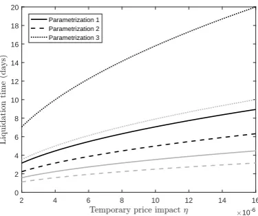
Figure 3 compares the time to liquidation assuming constant liquidation speed and no accruing interest,τ(s, z), with the actual average time to liquidation,T(Z = 0), which was computed based on 10,000 simulations. The initial block order size is fixed at z= 100 corresponding to 100,000 shares. The time to liquidation increases with stronger temporary price impactη and the actual actual time to liquidation is longer thanτ(s, z).
Figure 4 shows 10,000 simulations of the liquidation with s = z = 100 and η = 7.5×10⁻⁶ calibrated from Breen et al. (2002). All lines are shown until the (stochastic) time of liquidation,T(Z = 0), is reached. In the first column, we observe that, with each of the parameter sets, the execution time increases when the asset price is falling. On average, the execution takes 6.17, 4.36 and 13.80 days for the three parametrizations in Table 1, respectively.
0 0.01 0.02 0.03 0.04 0.05 0.06 0.07 0.08 0.09 0.1 x 0 0.02 0.04 0.06 0.08 0.1 0.12 0.14 I ( s; z ) = 1 ! u1 ( < 2x ) = ( < 2x ) Parametrization 1 Parametrization 2 Parametrization 3 (a)
0 0.01 0.02 0.03 0.04 0.05 0.06 0.07 0.08 0.09 0.1
x 0 0.5 1 1.5 2 2.5 3 3.5 = ( s; z ) = 2 x = (1 ! u
0 1(
< 2x )) Parametrization 1 Parametrization 2 Parametrization 3 (b)
Figure 2: (a) Relative implementation shortfall; (b) Time to liquidation assuming constant liquida-tion speed and no accruing interest, for three parametrizaliquida-tions in Table 1.
9. Conclusions
We have analyzed optimal liquidation of an asset whose unaffected price drifts downwards, while assuming that short sales of the asset are ruled out and the liqui-dation causes a linear temporary adverse price impact. In this setting the liquiliqui-dation time horizon becomes stochastic and is determined endogenously as part of the op-timal liquidation strategy. We have recovered a classical result from the martingale case whereby optimal liquidation always leads to implementation shortfall, in con-trast to previous studies using a fixed time horizon. While the ‘raw’ impact is linear the optimized impact is asymptotically proportional to the square root of the total volume of the order. This conclusion is well supported by empirical evidence.
The HJB equation of the new optimization gives rise to a boundary value problem whose degree of singularity is not covered in the existing literature. We have proposed a numerical scheme that overcomes the singularity and we have provided detailed theoretical analysis of the mixed boundary singular PDE our numerical scheme is based on.
For simplicity our work leaves out permanent impact and considers only linear utility. We have shown in Section 2 that in the martingale case with linear utility function the temporary and permanent impacts do not interact. In a drifting market there will be some degree of interaction, but for reasons given in Section 2 we suspect it to be rather weak. The precise nature of this interaction remains an intriguing area for future research.
Acknowlegements: We would like to thank M. Fila, P. Pol´aˇcik, P. Quittner and M. Winkler for advice concerning Sections 7 and 8. We are grateful to two anonymous referees for detailed comments and to participants of the London
[image:28.595.109.494.140.312.2]2 4 6 8 10 12 14 16
Temporary price impact2 #10-6
0 2 4 6 8 10 12 14 16 18 20
L
iq
u
id
a
ti
o
n
ti
m
e
(d
ay
s)
[image:29.595.207.395.139.296.2]Parametrization 1 Parametrization 2 Parametrization 3
Figure 3: Actual average time to liquidation,T(Z = 0), based on 10,000 simulations (black lines) and approximate time to liquidation, assuming constant liquidation speed,τ(z, s), (grey lines), for three parametrizations in Table 1 and changing values of the temporary price impact parameterη.
ematical Finance Seminar for their feedback. P. Brunovsk´y thankfully acknowledges support of VEGA grant Nr. 1/0319/15. Thanks also go to V ´UB Foundation for its support of A. ˇCern´y’s semester visit of Comenius University in Bratislava during which this research was initiated.
References
Almgren, R., Chriss, N., 2000. Optimal execution of portfolio transactions. Journal of Risk 3, 5–39. URLhttp://dx.doi.org/10.21314/JOR.2001.041
Almgren, R., Thum, C., Hauptmann, E., Li, H., 2005. Equity market impact. Risk 18 (7), 57–62. Anderson, B. D. O., Moore, J. B., 1989. Optimal Control: Linear Quadratic Methods. Prentice-Hall
International.
Ankirchner, S., Blanchet-Scalliet, C., Eyraud-Loisel, A., 2016. Optimal portfolio liquidation with additional information. Mathematics and Financial Economics 10 (1), 1–14.
URLhttp://dx.doi.org/10.1007/s11579-015-0147-3
Ankirchner, S., Kruse, T., 2013. Optimal trade execution under price-sensitive risk preferences. Quantitative Finance 13 (9), 1395–1409.
URLhttp://dx.doi.org/10.1080/14697688.2012.762613
Auzinger, W., Koch, O., Kofler, P., Weinm¨uller, E., 1999. The application of shooting to singular boundary value problems. Technical Report 126/99, Vienna University of Technology.
Bernstein, S., 1904. Sur certaines ´equations diff´erentielles ordinaires du second ordre. Comptes Rendus de l’Acad´emie des Sciences 138, 950–951.
Bershova, N., Rakhlin, D., 2013. The non-linear market impact of large trades: evidence from buy-side order flow. Quantitative Finance 13 (11), 1759–1778.
URLhttp://dx.doi.org/10.1080/14697688.2013.861076
Bertsimas, D., Lo, A. W., 1998. Optimal control of execution costs. Journal of Financial Markets 1 (1), 1–50. URLhttp://doi.org/10.1016/S1386-4181(97)00012-8
Breen, W. J., Hodrick, L. S., Korajczyk, R. A., 2002. Predicting equity liquidity. Management Science 48 (4), 470–483. URLhttp://www.jstor.org/stable/822546
(a) (b) (c)
(d) (e) (f)
[image:30.595.117.485.144.486.2](g) (h) (i)
Figure 4: Each row shows 10,000 simulations of the unaffected price S(t) (first column), inven-tory Z∗(t) (second column) and the optimal strategy v∗(t) (third column), for one of the three parametrizations in Table 1.
Brown, D. B., Carlin, B. I., Lobo, M. S., 2010. Optimal portfolio liquidation with distress risk. Management Science 56 (11), 1997–2014.
URLhttp://dx.doi.org/10.1287/mnsc.1100.1235
Brunovsk´y, P., ˇCern´y, A., Winkler, M., 2013. A singular differential equation stemming from an optimal control problem in financial economics. Applied Mathematics and Optimization 68 (2), 255–274.
URLhttp://dx.doi.org/10.1007/s00245-013-9205-5
Chen, J., Feng, L., Peng, J., 2015. Optimal deleveraging with nonlinear temporary price impact. European Journal of Operational Research 244 (1), 240–247.
URLhttp://dx.doi.org/10.1016/j.ejor.2014.12.034
Chen, J., Feng, L., Peng, J., Ye, Y., 2014. Analytical results and efficient algorithm for optimal portfolio deleveraging with market impact. Operations Research 62 (1), 195–206.
URLhttp://dx.doi.org/10.1287/opre.2013.1222
![Figure 1: (a) Solutions of BVPt[0,L] (dotted) and BVPt[0,L] (dashed) for L = 10 and different valuesof t](https://thumb-us.123doks.com/thumbv2/123dok_us/1367104.90087/25.595.114.492.139.308/figure-solutions-bvpt-dotted-bvpt-dashed-dierent-valuesof.webp)