Vector magnetometry exploiting phase-geometry effects in a double-resonance alignment magnetometer

Alignment Magnetometer

Stuart J. Ingleby,∗ Carolyn O’Dwyer, Paul F. Griffin, Aidan S. Arnold, and Erling Riis

Department of Physics, SUPA, Strathclyde University, 107 Rottenrow East, Glasgow, UK

(Dated: February 27, 2018)

Double-resonance optically pumped magnetometers are an attractive instrument for unshielded magnetic field measurements due to their wide dynamic range and high sensitivity. Use of linearly polarised pump light creates alignment in the atomic sample, which evolves in the local static magnetic field, and is driven by a resonant applied field perturbation, modulating the polarisation of transmitted light. We show for the first time that the amplitude and phase of observed first- and second-harmonic components in the transmitted polarisation signal contain sufficient information to measure static magnetic field magnitude and orientation. We describe a laboratory system for experimental measurements of these effects and verify a theoretical derivation of the observed signal. We demonstrate vector field tracking under varying static field orientations and show that the static field magnitude and orientation may be observed simultaneously, with experimentally realised resolution of 1.7 pT and 0.63 mrad in the most sensitive field orientation.

INTRODUCTION

Unshielded magnetic field measurements are a key technique in applications ranging from mineral survey-ing [1] to archaeology [2], and the development of com-pact fT-sensitivity magnetometers [3] may lead to signifi-cant advances in these applications. The measurement of gradients and curvature in an arbitrarily oriented static magnetic field are of critical importance. The practi-cal difficulties associated with developing portable cryo-genic systems for SQUID-based magnetometers makes the development of optically pumped atomic magne-tometers attractive. Unshielded optically-pumped gra-diometers have been demonstrated recently [4], using a double-resonance magnetometry scheme. In this work we demonstrate a technique for measurement of the full mag-netic field vector through the observation of geometry-dependent phase variations in the first- and second-harmonic components of the double-resonance signal.

In a double-resonance magnetometer, the evolution of atomic spins in a static fieldB~0is interrogated by

modu-lation at a frequencyωRF, with resonant response when

ωRFis equal to the atomic Larmor frequencyωL=γ|B0|,

whereγ is the gyromagnetic ratio for the probed atomic ground state. Modulation may take the form of oscil-lating pump light amplitude [5] polarisation [6] or fre-quency [7], or a small oscillating applied field B~RF [8].

For alkali metal vapour magnetometers operating in the geophysical field rangeωRF ≈ O(2π·100 kHz), a

conve-nient frequency range for digitization and software signal analysis, making double-resonance magnetometry a use-ful technique for uncompensated, portable, unshielded magnetometry, combining high dynamic range and high sensitivity. In order to develop techniques for compact sensors of low cost and power consumption, we use a single monochromatic pump-probe laser beam and

ap-ply a small magnetic field perturbation to resonantly drive atomic spin precession. The precessing atomic spins modulate the optical activity of the atomic cell and are detected by measurement of the polarisation of transmit-ted light.

Double-resonance sensors have been used widely in scalar field measurements for many years [9, 10]. Lock-ingωRF toωLusing the dispersive component of the de-modulated signal response allows|B0| to be determined

readily. However, this technique requires that the demod-ulation phase be seta priori and yields only information on the magnitude ofB~0. In addition, signal amplitude

in double-resonance magnetometry is highly dependent on the orientation ofB~0 relative toB~RF and the axis of

light propagation. Orientations of B~0 with zero signal

amplitude are known asdead-zones. We note that mea-surement schemes for dead-zone reduction or dead-zone free magnetometry have been demonstrated successfully [11]. In this paper we demonstrate a sensor configuration and analysis scheme for determination ofB~0 orientation

from the measured phases of the signal contributions ob-served at ωRF and 2·ωRF. We show that the detected

signal can be analysed using an atomic alignment model to determine the magnitude and orientation ofB~0,

allow-ing the full field vector to be inferred.

Various other schemes for vector atomic magnetom-etry have been demonstrated, including zero-field sen-sors [12, 13], orthogonal probe lasers [14], orthogonal pump lasers [15], measurement of EIT (electromagneti-cally induced transparency) resonances [16] and applica-tion of significant slowly varying B~0 perturbations [17–

19]. The scheme demonstrated here complements these approaches by addressing some of their practical draw-backs. Zero-field techniques are well-suited for shielded measurements, but lack the dynamic range required for portable unshielded measurements, and additionally

FIG. 1. Schematic showing the geometry of the optical sys-tem and the laboratory (Lab), rotating-wave (RW) and anal-yser reference frames. The orientation of the static magnetic fieldB0~ is described by the spherical polar anglesθV andθL, and the oscillating magnetic field applied on thez-axis. The dashed lines show the linear light polarisation decomposed into orthogonal analysis components, whose intensity differ-ence is measured using a differential photodetector.

quire full-field compensation. The use of compensation coils, additional light frequencies or beams and addi-tional B~0 perturbations add significant hardware

over-heads and power requirements. We also wished to avoid vector magnetometry schemes requiring sequential mea-surements under varying field conditions, or observation of free induction decay signals, as these methods require longer sampling times and impose stringent upper limits on the achievable sensor bandwidth.

THEORY

A simple single-beam Mxmagnetometer configuration

is used, but the geometry of the static and modulating magnetic fields, atomic sample and analysis optics is crit-ical to the analysis technique and is shown in detail in Figure 1. A half-waveplate is used to balance the de-tector by rotating the linear polarisation of transmitted light by 45◦, meaning that light which is x-polarised at the atoms is equally split by the analyser. The observed differential signal is equal to the difference in transmis-sion of the two orthogonal analysis components separated by the polarising beam splitter.

The absorption of linear polarisation states by the atomic sample varies with the evolution of polarisation alignment moments in the sample. If the light polari-sation axis defines the quantipolari-sation axis, then the light

absorption coefficient is proportional to

κ∝√A0 3m0,0−

r

2

3A2m2,0, (1)

where the analysing powers A0 and A2 depend on the

hyperfine states coupled by the light, and the multipole moments mk,q describe the polarisation of the atomic sample [20, 21].

We can therefore write the observed signal as the dif-ference between the absorption of the two analyser lin-ear polarisation states, as shown in Figure 1. Since the terms inm0,0are invariant under rotations, and cancel in

subtraction, the observed differential signal f(t) is pro-portional to

f(t) =m02,0(t)−m002,0(t), (2)

wherem0 and m00 denote multipole moments describing atomic polarisation alignment in the two orthogonal anal-ysis frames. Rotation [22] of these moments into the lab-oratory frame yields

f(t) =

q

3

2(m2,−1(t)−m2,1(t)). (3)

The dynamic evolution of multipole moments under the static fieldB~0 and perturbing fieldB~RF can be

de-rived from the Lioville Equation [23]. Steady-state os-cillating solutions can be found by setting ˙mk,q = 0 in a frame co-rotating with the perturbing field B~RF (the

rotating wave frame, denotedmRW

k,q). If the RW frame is chosen such that B~RF(t = 0) is in the−xdirection, we

can follow the method of [20], finding solutions formRW 2,q using

i

Γm˙

RW

2,q =Mqq0mRW_2,q0+im¯RW_2,q, (4)

where Γ is an isotropic spin relaxation rate, ¯mRW 2,q are moments describing equilibrium magnetisation in the ab-sence of the RF field, and

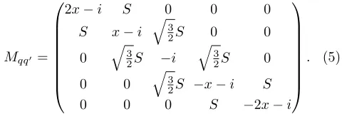
Mqq0 =         

2x−i S 0 0 0

S x−i q3₂S 0 0

0

q

3 2S −i

q

3

2S 0

0 0 q3₂S −x−i S

0 0 0 S −2x−i

         . (5)

For convenience we define the dimensionless quantities

x= (ωRF−ωL)/Γ andS =γBRF⊥ /Γ, where BRF⊥ is the

component ofB~RF perpendicular toB~0 andγ is the

gy-romagnetic ratio for the Cs 62_S

1/2(F = 4) ground state.

and the equilibrium magnetisation ¯mRW_k,q is aligned with the static field vector B~0 (i.e. m¯RWk,q = ¯m for q = 0,

¯

mRW

k,q = 0 otherwise). The magnitude of ¯m is propor-tional to the projection of mRW2,0 onto mPUMP2,0 , where

mPUMP

k,q are defined in a frame where the quantisation axis is parallel to the polarisation axis of the pump light.

Steady-state ˙mRW

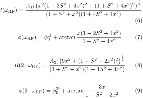
2,q = 0 solutions for mRW2,q can be found, and so m2,q(t) found by rotation [22]. Substi-tution into (3) yieldsf(t), with terms ine0·iωRFt_,e1·iωRFt

ande2·iωRFt_{. Similarly to [20], we write the amplitudeR}

and phase φ of the oscillating responses to B~RF in the

following form;

R(ωRF) =

A1f x2(1−2S2+ 4x2)2+ (1 +S2+ 4x2)2

12

(1 +S2_+x2_{)(1 + 4S}2_{+ 4x}2₎

(6)

φ(ωRF) =φ1f0 + arctan

x(1−2S2_{+ 4x}2₎

1 +S2_{+ 4x}2 (7)

R(2·ωRF) =

A2f 9x2+ (1 +S2−2x2)2

1₂

(1 +S2_+x2_{)(1 + 4S}2_{+ 4x}2₎ (8)

φ(2·ωRF) =φ2f0 + arctan

3x

1 +S2_−2x2. (9)

The on-resonance amplitudeAand phaseφ0of the signal

vary withθL andθV as given in Equations 10-13.

A2_1f= ¯m2S2 (cosθV cosθL)2+ (cos 2θV sinθL)2 (10)

A2_2f= ¯m2S4 1

2sin 2θV sinθL

2

+ (sinθV cosθL)2

(11)

tanφ1f₀ = −mS¯ cosθV cosθL ¯

mScos 2θV sinθL

(12)

tanφ2f₀ = 2 ¯msinθVcosθL −m¯ sin 2θV sinθL

(13)

TEST SYSTEM

In order to obtain accurate data on the relation of double-resonance signal phase to B~0 orientation, a

shielded test system was used, reducing the effect of back-ground magnetic field noise and allowing fine control of

~

B0 orientation. The use of magnetic shielding also

al-lowed us to operate in a low-field regime (|B0| ≈200 nT),

in which the non-linear Zeeman splitting, which leads to systematic shifts in the observed magnetic resonance, is negligible compared to the natural linewidth of the mag-netic resonance.

FIG. 2. Schematic of the experimental system, showing ex-ternal cavity diode laser (ECDL), Glan-Thompson linear po-lariser (GT), magnetometer cell, five-layer mu-metal shield, three-axis Helmholtz coils, half-wave plate (λ/2), polaris-ing beam splitter (PBS), differential photodetector (DPD), low-noise coil driver (LNCD) and data acquisition system (DAC/ADC). The data acquisition system is controlled us-ing a PC (not shown).

Figure 2 shows the test system used, and a detailed hardware description can also be found in [25]. A spher-ical room temperature cell of 28 mm diameter contain-ing133_{Cs [26] is contained within a five-layer mu-metal}

shield. Optical access is via a 10 mm diameter axial port and the local static magnetic field at the cellB~0 is

controlled using three pairs of Helmholtz coils driven by six independent software-controlled current supplies. A Helmholtz coil pair on the z-axis is used to apply the oscillating perturbation field B~RF. A 1.4 MHz 16-bit

DAC/ADC (National Instruments PCIe-6353) is used to generateB~RF and digitise the differential photodetector

signal. Demodulation is carried out in software.

An external-cavity diode laser (New Focus Vortex 6800) provides optical pump/probe light resonant with the 62_S

1/2 (F = 4) to 62P1/2 (F = 3) transition of an

external 133_{Cs reference cell. This light is linearly}

po-larised along the x-axis prior to the magnetometry cell using a Glan-Thompson polariser.

A single magnetic resonance measurement is conducted as follows; following the establishment of the desired

~

B0 using the calibrated coil system, an RF modulation

signal is generated using the digital-analogue converter. The RF modulation frequency ωRF is chirped in finite

steps. The detector signal response to the modulation signal is synchronously digitised, and a sample segment from eachωRF step demodulated to obtain the in-phase

X(ωRF),X(2·ωRF) and quadratureY(ωRF),Y(2·ωRF)

responses. The sample segments are timed such that each commences in phase withB~RF and contains an

in-teger number ofB~RF periods. Sample segment length is

kept approximately constant for allωRF, and each

FIG. 3. A measured and fitted magnetic resonance, taken with |B0| = 200 nT applied at θV = 118◦ , θL = 101◦ and |BRF| = 1.5 nT. A total of 150 segments of data are taken, with segment sample time 20 ms. Left: amplitude (R) and phase (φ) components of the first-harmonic de-modulated signal. Right: amplitude (R) and phase (φ) of the second-harmonic demodulated signal. The data are fit-ted with Equations 6 - 9, yielding ωL = 2π· 699.60(2) Hz, Γ = 12.1(1) Hz, A1f = 107.4(7) mV, φ1f0 = 0.9672(9) π.rad, φ2f0 =−0.383(6)π.rad and Ω = 2.89(8) Hz.

duration, to allow the steady-state oscillating response toB~RF(ωRF) to be measured.

Figure 3 shows measured signal amplitude R ≡ √

X2_+Y2 _{and phaseφ≡arctan(X/Y) for data}

demod-ulated at ωRF and 2·ωRF. Least-squares fits of

Equa-tions 6 - 9 (these resonance shapes and the underlying physical model are described in detail below) are used to estimate the Larmor frequency ωL, spin relaxation rate Γ, on-resonance signal amplitude A and phase φ0, and

magnetic Rabi rate Ω.

STATIC FIELD CALIBRATION

To achieve precise control ofB~0, allowing measurement

of orientational effects, the static field generating coils are calibrated by measurement of the Larmor frequency un-der varying orientations of the applied field. The method for initial coil calibration is described in [25]. For a given application of the applied fieldB~APP_{, the magnitude of}

the measured field|BMEAS|=ωL/γ is determined by fit-ting Equations 6 - 9 to the demodulated data R(ωRF)

andφ(ωRF).

Following the initial calibration, fine coil calibration is carried out by orienting B~APP _{in 1646 orientations,}

spaced with equal angular coverage over the full solid angle, and performing a weighted fit to the observed dis-tribution of|BMEAS|with

|BMEAS|=

s X

i

(i+aiBiAPP)2, (14)

where is the background field andais a dimensionless coil calibration factor. The calibration and offset of each

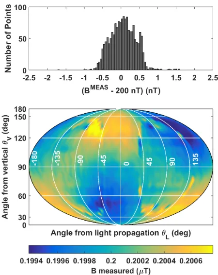
FIG. 4. Measured magnitude ofB0~ , determined from mea-surements ofωLat 1646 differentB0~ orientations, evenly cov-ering the full solid angle. Top: distribution of measured|B0|

around desired field magnitude of 200 nT. The RMS spread of|B0|is 302 pT.Bottom: angular distribution of|B0|.

coil can then be corrected by the best-fit parametersai and i. The uncertainties in the fit δa and δ can be used to estimate the tolerances in the magnitude and orientation ofB~0,δB0andδθ, by assuming that the total

field uncertainty, estimated byδB0 = |δ|+|B0||δa|, is

perpendicular toB~0, yieldingδθ≈δB0/|B0| forδB0

|B0|.

Table I gives the calibration parameter uncertainties for the final coil calibration, and Figure 4 shows the mea-sured value of|B0| over the full solid angle for the

sub-sequent field vector measurements. In order to render heading-error effects due to non-linear Zeeman splitting negligible, a field magnitude of |B0| ≈ 200 nT is used

throughout. From the calibration uncertainties we esti-mate tolerances of δ|B0| = 54 pT and δθ = 0.27 mrad.

The RMS spread of observed magnitudesδ|B0|RM S from

Figure 4 is 302 pT. Although the difference between

δ|B0|andδ|B0|RM S is indicative of some remaining

non-normal (i.e. anisotropic, systematic) contributions toB~0

discrepancies, we can still be confident that B~0 can be

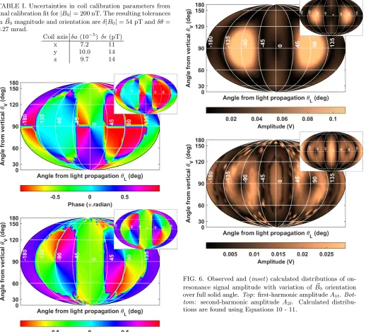
TABLE I. Uncertainties in coil calibration parameters from final calibration fit for|B0|= 200 nT. The resulting tolerances inB0~ magnitude and orientation areδ|B0|= 54 pT andδθ= 0.27 mrad.

Coil axis δa(10−5_{) δ(pT)}

x 7.2 11

y 10.0 14

z 9.7 14

FIG. 5. Observed and (inset) calculated distributions of on-resonance signal phase with variation of B0~ orientation over full solid angle. Top: first-harmonic phase φ1f0.

Bot-tom: second-harmonic phase φ2f

0. Calculated distributions are found using Equations 12 - 13.

VECTOR FIELD MEASUREMENTS

Equations 10 - 13 indicate a strong dependency be-tween the on-resonance signal components and the orien-tation ofB~0. Using the calibrated field control described

above, automated scans of B~0 were carried out. Each

scan consists of 1646 orientations ofB~0, spread over the

FIG. 6. Observed and (inset) calculated distributions of on-resonance signal amplitude with variation ofB0~ orientation over full solid angle. Top: first-harmonic amplitudeA1f. Bot-tom: second-harmonic amplitudeA2f. Calculated distribu-tions are found using Equadistribu-tions 10 - 11.

full solid angle with approximately even angular distribu-tion. At eachB~0 orientation, a magnetic resonance

mea-surement was carried out, and a fit to the resulting data using Equations 6 - 9 used to obtain best-fit values and uncertainties forφ1f0,φ2f0,A1fandA2f. The results of this

measurement are shown in Figures 5 - 6. Good agreement was found between the on-resonance signal components in the measured data and Equations 10 - 13.

We note the dependence of the first- and second-harmonic on-resonance signal phasesφ1f

0 andφ2f0 on the

orientation ofB~0. From Equations 12 - 13 we can derive

Equations 15 - 16 forθV andθL.

tan2θV = 1− tanφ2f

0

tanφ1f 0

FIG. 7. Measured and set magnetic field magnitude and orientation for a wide range ofB0~ orientations. Observed values and uncertainties forθV andθLare calculated fromφ1f0 andφ2f0 using Equations 15 and 16. The point of best angular resolution is measured at (|B0|= 199.8445(17) nT , θV = 100.986(27)◦,θL= 118.198(24)◦). The inset in the lower left corner shows the contour described by successiveB~APPorientations, plotted using the same projection as Figures 5 and 6.

tanθL=

−cosθV cos 2θV tanφ1f0

(16)

By measuring the resonant response of the detector signal, demodulating to obtain the first- and second-harmonic signal amplitude and phase, and fitting to de-termine the Larmor frequency and on-resonance phases, we can calculateθV andθL and make a full-vector mea-surement ofB~0.

Figure 7 shows calculatedθV andθL for a range ofB~0

orientations defined using the calibrated Helmholtz coil system. The range of orientations is shown as an inset to Figure 7 and was chosen to scan over the zone of high signal amplitude around the light polarisation (x-) axis. At each point the first- and second-harmonic resonance responses are measured for a range ofxand fitted using Equations 6 - 9. The on-resonance phasesφ1f

0 andφ2f0 are

free parameters in this model, and the fit uncertainties are propagated through Equations 15 - 16 to give the uncertainties inθV andθL. The point of highest observed angular resolution has uncertainties of δ|B0| = 1.7 pT,

δθV = 0.027◦, δθL = 0.024◦, giving an overall angular resolution at this point ofδθ= 0.036◦ (0.63 mrad).

CONCLUSIONS

The measurement of complementary field orienta-tion informaorienta-tion using a hitherto-scalar double-resonance magnetometry technique has clear potential for impact in practical measurements of arbitrarily oriented fields. Ex-isting three-axis magnetometer data is often transformed to derive data on field magnitude, declination and incli-nation. In this work we demonstrate a scheme for inde-pendent measurement of the field vector in this spher-ical polar basis, while also exploiting the precise and accurate measurement of field magnitude possible with the double-resonance technique. The single-beam, RF-modulated detection scheme used is imminently suitable for scalable, portable devices.

The data shown in Figure 7 demonstrate resolution of the magnetic field magnitude at the pT-level and mag-netic field orientation at the sub-mrad level. The vari-ation of the measured field magnitude and orientvari-ation from the expected field magnitude (200 nT) and orien-tation (solid lines) exposes residual calibration errors in the Helmholtz coil system, which can setB~0 with

the-ory and observed in Figure 5 are not called into question, but a more stringent test of the absolute accuracy of the field orientation measurement will require improvements to the hardware of the Helmholtz coil system, including improved design tolerances on the coil geometry (cur-rently at the 100-micron level), improved linearity of the coil current drivers and associated DACs and increased detector signal-to-noise, which would also improve the resolution of both the calibration and vector field data.

The double-resonance scheme presented also has some drawbacks in the implementation of practical sensors, which may form the context for further work. We ob-serve dead-zones, both where signal amplitude falls to zero (dark regions in Figure 6) and angular dead-zones; orientations for which the observed signal phase has no variation with field orientation∂φ0/∂θ= 0. These

angu-lar dead-zones do not necessarily coincide with the signal-amplitude dead-zones, and can be seen in Figure 7 as angular data points with very high uncertainties. A fur-ther drawback of this technique is the requirement that magnetic detuning x be measured independently from phases-on-resonance φ1f₀ and φ2f₀. In this work we met this requirement at the expense of bandwidth by mea-suring and fitting a ωRF frequency sweep at each data

point.

To conclude, we have demonstrated a new analysis technique for double-resonance alignment try that can be used to implement vector magnetome-try using a scalar device. No additional lasers or field-generating coils are required, and the vector field sen-sitivity achieved using this technique could be further enhanced by rapid independent measurement of x, φ1f0

andφ2f

0, allowing the field vectorB~0(t) to be determined

with high bandwidth.

ACKNOWLEDGEMENTS

The authors would like to thank Prof. Antoine Weis and Dr. Victor Lebedev of Fribourg University for supplying the Cs vapour cell used in this work. This work was funded by the UK Quantum Technology Hub in Sensing and Metrology, EPSRC (EP/M013294/1). The data shown in this paper is available for download at http://dx.doi.org/10.15129/5f63cec2-e674-4e42-b923-7550e28d860f.

∗

[email protected]

[1] M. N. Nabighian, V. J. S. Grauch, R. O. Hansen, T. R. LaFehr, Y. Li, J. W. Peirce, J. D. Phillips, and M. E. Ruder, Geophysics70, 33ND (2005).

[2] E. Ben-Yosef, M. Millman, R. Shaar, L. Tauxe, and O. Lipschits, Proceedings of the National Academy of Sciences114, 2160 (2017).

[3] D. Sheng, A. R. Perry, S. P. Krzyzewski, S. Geller, J. Kitching, and S. Knappe, Applied Physics Letters 110, 031106 (2017).

[4] G. Bevilacqua, V. Biancalana, P. Chessa, and Y. Dancheva, Applied Physics B: Lasers and Optics122, 103 (2016), arXiv:1601.06938 [physics.ins-det].

[5] S. Pustelny, W. Gawlik, S. M. Rochester, D. F. J. Kim-ball, V. V. Yashchuk, and D. Budker, Phys. Rev. A74, 063420 (2006), arXiv:0606257 [physics].

[6] E. Breschi, Z. D. Gruji´c, P. Knowles, and A. Weis, Appl. Phys. Lett. 104 (2014), 10.1063/1.4861458, arXiv:arXiv:1312.3567v1.

[7] R. Jim´enez-Mart´ınez, W. C. Griffith, Y. J. Wang, S. Knappe, J. Kitching, K. Smith, and M. D. Prouty, IEEE Trans. Instrum. Meas.59, 372 (2010).

[8] T. Zigdon, A. D. Wilson-Gordon, S. Guttikonda, E. J. Bahr, O. Neitzke, S. M. Rochester, and D. Budker, Opt. Express18, 25494 (2010), arXiv:1008.3000.

[9] W. E. Bell and A. L. Bloom, Phys. Rev. Lett. 6, 280 (1961).

[10] A. L. Bloom, Appl. Opt.1, 61 (1962).

[11] A. Ben-Kish and M. V. Romalis, Phys. Rev. Lett.105, 193601 (2010).

[12] S. Pradhan, Review of Scientific Instruments87, 093105 (2016).

[13] S. J. Seltzer and M. V. Romalis, Applied Physics Letters 85, 4804 (2004).

[14] S. Afach, G. Ban, G. Bison, K. Bodek, Z. Chowd-huri, Z. D. Gruji´c, L. Hayen, V. H´elaine, M. Kasprzak, K. Kirch, P. Knowles, H.-C. Koch, S. Komposch, A. Kozela, J. Krempel, B. Lauss, T. Lefort, Y. Lemi`ere, A. Mtchedlishvili, O. Naviliat-Cuncic, F. M. Piegsa, P. N. Prashanth, G. Qu´em´ener, M. Rawlik, D. Ries, S. Roc-cia, D. Rozpedzik, P. Schmidt-Wellenburg, N. Severjins, A. Weis, E. Wursten, G. Wyszynski, J. Zejma, and G. Zsigmond, Opt. Express23, 22108 (2015).

[15] B. Patton, E. Zhivun, D. C. Hovde, and D. Budker, Phys. Rev. Lett.113, 013001 (2014).

[16] K. Cox, V. I. Yudin, A. V. Taichenachev, I. Novikova, and E. E. Mikhailov, Phys. Rev. A83, 015801 (2011). [17] A. J. Fairweather and M. J. Usher, Journal of Physics E:

Scientific Instruments5, 986 (1972).

[18] L. Lenci, A. Auyuanet, S. Barreiro, P. Valente, A. Lezama, and H. Failache, Phys. Rev. A 89, 043836 (2014).

[19] A. K. Vershovskii, M. V. Balabas, A. ´E. Ivanov, V. N. Kulyasov, A. S. Pazgalev, and E. B. Aleksandrov, Tech-nical Physics51, 112 (2006).

[20] A. Weis, G. Bison, and A. S. Pazgalev, Phys. Rev. A74, 033401 (2006).

[21] M. Auzinsh, D. Budker, and S. Rochester,Optically Po-larized Atoms (Oxford University Press, 2010).

[22] M. A. Morrison and G. A. Parker, Australian Journal of Physics40, 465 (1987), arXiv:arXiv:1011.1669v3. [23] S. J. Ingleby, C. O’Dwyer, P. F. Griffin, A. S. Arnold,

and E. Riis, Phys. Rev. A96, 013429 (2017).

[24] S. M. Rochester, M. P. Ledbetter, T. Zigdon, A. D. Wilson-Gordon, and D. Budker, Phys. Rev. A 85, 022125 (2012).

[25] S. J. Ingleby, P. F. Griffin, A. S. Arnold, M. Chouliara, and E. Riis, Rev. Sci. Instrum.88, 043109 (2017). [26] N. Castagna, G. Bison, G. Di Domenico, A. Hofer,