City, University of London Institutional Repository
Citation:
Rajarajan, M. & Yogachandran, R. (2017). Efficient Privacy-Preserving Facial
Expression Classification. IEEE Transactions on Dependable and Secure Computing, 14(3),
pp. 326-338. doi: 10.1109/TDSC.2015.2453963
This is the accepted version of the paper.
This version of the publication may differ from the final published
version.
Permanent repository link:
http://openaccess.city.ac.uk/12198/
Link to published version:
http://dx.doi.org/10.1109/TDSC.2015.2453963
Copyright and reuse: City Research Online aims to make research
outputs of City, University of London available to a wider audience.
Copyright and Moral Rights remain with the author(s) and/or copyright
holders. URLs from City Research Online may be freely distributed and
linked to.
Efficient Privacy-Preserving Facial Expression
Classification
Yogachandran Rahulamathavan,
Member, IEEE
, and Muttukrishnan Rajarajan,
Senior Member, IEEE
Abstract—This paper proposes an efficient algorithm to perform privacy-preserving (PP) facial expression classification (FEC) in the client-server model. The server holds a database and offers the classification service to the clients. The client uses the service to classify the facial expression (FaE) of subject. It should be noted that the client and server are mutually untrusted parties and they want to perform the classification without revealing their inputs to each other. In contrast to the existing works, which rely on computationally expensive cryptographic operations, this paper proposes a lightweight algorithm based on the randomization technique. The proposed algorithm is validated using the widely used JAFFE and MUG FaE databases. Experimental results demonstrate that the proposed algorithm does not degrade the performance compared to existing works. However, it preserves the privacy of inputs while improving the computational complexity by120times and communication complexity by31percent against the existing homomorphic cryptography based approach.
Index Terms—Privacy, security, facial expression, classification, encrypted domain.
F
1
I
NTRODUCTIONFacial expression classification (FEC) forms a critical capability desired by human-interacting systems that aim to be responsive to variations in the human’s emotional state [1]–[3]. Automatic recognition of FaEs can be an important component in human-machine interfaces, human emotion analysis and medical care. However, the task of automatically recognizing the various FaEs is challenging [4]–[6].
The FEC could be automated by establishing a com-puting infrastructure capable of executing machine learning algorithms and building a database of facial images with different expressions. These requirements may not achievable by small organizations. Even if we assume that the requirement can be met by organiza-tions, then they need a dedicated team to maintain the infrastructure which may not be necessary when cheaper computational power and services can be obtained from cloud providers. Hence, it is reasonable to assume that any organization can obtain the FEC as a service from cloud provider or any other modern computing infrastructure.
If the FEC is outsourced to modern computing in-frastructures then it involves third party servers who deliver FEC as a service via the Internet. Initially, the server sets up a database with training facial images from various expression classes and extracts the dis-criminative features of these images that correspond to each class in order to simplify the classification.
• Y. Rahulamathavan and M. Rajarajan are with the Information Secu-rity Group, School of Engineering and Mathematical Sciences, City University London, EC1V 0HB, London, U.K. (e-mails: [email protected] and [email protected]).
A client requesting the service would supply a test image whose expression it desires to recognize. In re-sponse the server extracts the discriminative features from the test image and compares them against the features of training images in order to find the test image’s expression.
However, due to privacy concerns, the client re-questing the service may not wish to disclose the contents of the facial image or the classification results (i.e., which expression is present in the current test facial image) to the server; while the server desires that the service does not leak out information to the client on the reference facial images that it holds in its database. As an example, a doctor may wish for her patients’ emotions to be automatically recognized (rather than manually as this will be time-consuming), through the aid of a FaE database hosted on a remote server. In order to address any privacy concerns that may result from revealing patient images without explicit consent, this should be performed without leaking the contents of the patients’ face images nor even the classification results to the server.
C1: develop a lightweight solution for FEC without
using computationally intensive cryptographic techniques
C2: at the same time achieve classification accuracy
equivalent to the accuracy of the conventional non-PP algorithm
The remainder of this paper is organized as follows: We review the related works in Section 2. Notation and mathematical tools required for our algorithm are given in Section 3. In Section 4, we describe the conventional FEC algorithm (i.e., without privacy requirements). In Section 5, we propose the efficient algorithm to achieve privacy during the classifica-tion followed by security and privacy analysis. Per-formance of the proposed algorithm is analyzed in Section 6. Conclusions are discussed in Section 7.
2
R
ELATED WORKSThere are several classification algorithms developed in pattern recognition and machine learning for var-ious applications [7]. Few of them in the literature have been redesigned for PP classification ( [8]–[15], [29] and references therein). Majority of these are de-veloped for distributed setting where different parties hold parts of the training database and securely train a common classifier without each party needing to disclose its own training data to other parties [9], [10]. The work in [9] proposed for the first time a strongly privacy-enhanced protocol for support vec-tor machine (SVM) using cryptographic primitives whereas the authors assumed that the training data is distributed. Hence, in order to preserve the privacy they developed a protocol to perform secure kernel sharing, prediction and training using secret sharing and homomorphic encryption techniques. At the end of the training, each party will hold a share of the secret. In the testing phase, all parties collaboratively perform the classification using their shared secrets. At the end of the protocol, each party will hold the share of the predicted class label.
PP data classification algorithms suitable for client-server model were studied in [8], [11]–[15], [29]. The client-server model substantially reduces the compu-tational and communication overhead to the client since s/he needs to interact with only one server compared to the distributed setting. The work in [8] proposes a PP face recognition algorithm using cryptographic techniques. Outsourcing the clinical decision support system to the third-party server without violating the client’s privacy was studied in [15]. Similarly several plain domain classification algorithms were redesigned in [11]–[14] to perform PP classifications.
The PP algorithm for FEC algorithm was studied in [29]. The work in [29] is a variant of [8]. Even though, at high level, there are similarities between [8] and [29] in the PP computation part, there are significant
differences between both the schemes. The scheme in [8] uses principal component analysis (PCA) for feature extraction and then nearest neighbor (NN) classifier. One problem that can be associated with PCA is that it is very sensitive to variations in expres-sion, illumination, occlusion etc. In order to overcome this drawback, Belhumeur et. al proposed a technique called Fisher Linear Discriminant Analysis (FLDA) in [23] and showed that the method in [23] has lower error rates that than PCA based technique. However, FLDA tends to give undesired results if image sam-ples in a particular class have many local means (i.e., a multimodal class). In that case FLDA cannot preserve the discriminative features of that particular class. Local Fisher discriminant analysis (LFDA) has been proposed to overcome drawbacks of FLDA [25]. Due to this, [29] considers LFDA instead of PCA.
The work in [29] achieves the privacy requirements by masking the test image and results using Paillier homomorphic encryption [16]. Homomorphic cryp-tosystems such as Paillier are public key cryptosys-tems and use large keys for encryption and decryption [16]. This involves computationally intensive opera-tions such as exponentiation of very large numbers. On the other hand, the homomorphic encryption used for data classification schemes only perform limited number of operations in the encrypted domain (either addition or multiplication). Hence, more number of interactions between the client and server is required to obtain the result.
In contrast to all of these works, we propose a lightweight PP FEC protocol based on randomization technique. The protocol relies only on multiplication and addition. However, we show later in this pa-per that the new protocol achieves the privacy re-quirements without degrading the classification per-formance while improving the computational and communication complexity compared to the existing work.
3
PRELIMINARIES
We use boldface upper and lower case letters for matrices and vectors;(.)T denotes the transpose oper-ator;∥.∥2 the Euclidean norm; ⌊.⌉ the nearest integer
approximation;⊗denotes the Kronecker product. The modular reduction operator is denoted by mod. vec
denotes vectorization operation which converts the matrix into a column vector.
3.1 Kronecker product and identities
In mathematics, the Kronecker product, denoted by ⊗, is an operation on two matrices of arbitrary size resulting in a block matrix. This product satisfies the following two identities [17] (notations A, B, C, D, andXto be used to define matrices with appropriate sizes):
2. (A⊗B)(C⊗D) = (AC)⊗(BD)
3.2 Information-theoretic security
A security algorithm is information-theoretically se-cure if its security is derived purely from information theory. The concept of information-theoretically se-cure communication was introduced in1949by Amer-ican mathematician Claude Shannon, who used it to prove that the one-time pad system archives perfect security subject to the following two conditions [18]:
1. the key which randomizes the data should be random and should be used only once
2. the key length should be at least as long as the length of the data
If any algorithm randomizes its parameter and sat-isfies the above conditions then the parameters can-not be unmasked by an adversary even when the adversary has unlimited computing power e.g., if the message space and random space are equal to 1024−bits thenpriorprobability (probability for a par-ticular message out of 21024 possible messages) and posteriorprobability (probability of inferring/mapping a message in random domain to a message domain) are equal i.e., there is no advantage for an adversary to get higher posterior probability than prior probability.
3.3 Privacy-preserving secure two-party compu-tation
This computation will be exploited to perform secure operation between two parties. Let us assume one party i.e., client knows a vectora and another party i.e., server knows a vectorband scalarr. Both want to interact with each other to computeaTb+r. However, the outcomeaTb+rmust be known only to the client.
To compute r +aTb in private, we extend the PP
scalar multiplication algorithm in [19] . The complete algorithm is presented in Table 1.
Let us assume that the client’s inputais composed of integers while the server’s inputbis composed of floating points. Since we use integer random numbers, the server converts the elements inbinto integers by scaling and nearest integer approximation operation. This is a valid operation since we scale the vector,b, and r by a large scalar, s, before computation (i.e.,
s.r+aT⌊sb⌉) and divide the outcome by the same
scaling factor s (i.e., 1
s(s.r +a
T⌊sb⌉) ≈ r+ aTb).
Initially, the client adds different random values to each of the elements in a as shown in Steps 7 to 10 in Table 1. Now the server executes the Steps from14 to 21 and returns the outcome to the client. In Step 21, the server adds random numbers.r.α2to∑l
i=1Di.
[image:4.567.289.525.42.496.2]Theorem 1: The above two-party protocol is information-theoretically secure i.e., the server cannot infer the elements in client’s input vector a and the client will only learn the final result but not the elements in sever’s input vectorbnorr.
TABLE 1
PP Secure Two-party Computation Algorithm to Computer+aTbPrivately.
1.Input by Client:a= [a1, . . . , al]T, wherel <216,
{(ai)∀i} ∈Zo1 witho1≤2 10
Input by Server:r,⌊s.b⌉= [⌊s.b1⌉, . . . ,⌊s.bl⌉]T,
where{s.r, (bi)∀i} ∈Zo2 witho2≤240
2.Output:r+1
s(⌊sa⌉ Tb)
(known only to the client)
Client first performs the following operations
3. choose primesα,β, where|α|= 80bits and
β>(l.o1.o2+o2+ 1).α2, e.g.,|β|>226bits ifl= 216
4. setK= 0 and chooselpositive
random integers(c1, . . . , cl)
such thato2.
∑l
i=1ci< α−o2.land|ci|<24bits
5. foreach elementbi∈bdo
6. choose random integerzi, computezi.βsuch that
|zi.β| ≈1024bits, and calculateki=zi.β−ci
7. ifbi>0thencompute
8. Ci=ai.α+ci+zi.β,K=K+ki
9. else ifbi= 0thencompute
10. Ci=ci+zi.β,K=K+ki
11. end if
12. end for
13. send(α, C1, C2, . . . , Cn)to the server
Now server executes the following operations
14. foreach elementbi∈bdo
15. if⌊s.bi⌉>0thencompute
16. Di=⌊s.bi⌉.α.Cii.e., ifai>0
→Di=⌊s.bi⌉.ai.α2+⌊s.bi⌉.α.ci+⌊s.bi⌉.α.zi.β
ifai= 0→Di=⌊s.bi⌉.α.ci+⌊s.ai⌉.α.zi.β
17. else ifbi= 0thencompute
18. Di=Cii.e., ifai>0→Di=ai.α+ci+zi.β
ifai= 0→Di=ci+zi.β
19. end if
20. end for
21. computeD=s.r.α2+∑li=1Di and
returnD to the client
Now client performs the following operations
22. computeE=D+K mod β
23. return E−(E mod αs.α2 2) which is equal to
r+1 s(⌊sb⌉
Ta)≈aTb+r
24.end procedure
Proof: To validate the security we consider both the client and server are honest-but-curious i.e., they will follow the procedures but try to learn about each other’s input, intermediate values and result. Let us show that the algorithm in Table 1 is information-theoretically secure for the following two cases.
Case I–Honest-but-curious Server
In Table 1, the client randomizes his inputs ai, i =
1, . . . , lby 712-bits of freshly generated random inte-gers zi, i = 1, . . . , l and sends Ci, i = 1, . . . , l to the
server (see Steps3to13). The server is curious to infer the clients data ai from Ci. The server can compute
theprioriprobabilities of random integerzi and data ai based on the underlying stochastic process as well
as the posteriori probabilities of the various possible
ai and keysci+ziβ which might have produced Ci.
integers are fresh, then the server can only compute identical priory and posteriori probabilities, hence the client’s data is information-theoretically secure. In Section 5.3 we show that the size of the client’s input data is always less than1024−bits.
Case II–Honest-but-curious Client
As shown in the Steps 14 to 21 in Table 1, the server’s input datas.bi, i= 1, . . . , lis multiplied with
corresponding ai and then the results were added
to get ∑li=1s.bi.ai in the randomized domain. The
curious client wants to infer∑li=1s.bi.aior the servers
input from the result. The outcome is randomized by
s.r where r is freshly generated random value (we avoided α2 in here for brevity). In fact the server
hides∑li=1bi.ai usings.rfrom the curious client. As
explained previously, the server can secure∑li=1bi.ai
information-theoretically if the size of the random integer r is greater than the size of the outcome ∑l
i=1bi.ai. In Section 5.3, we show that the server can
determine the size of∑li=1bi.aiso that it can generate
larger integers.rin order to achieve the information-theoretic security.
Theorem 2: The algorithm in Table 1 is not vulnera-ble to overflow errors.
Proof: Let us assume that elements in vectors a, ⌊s.b⌉, ands.ri take maximum possible values. Let us
denote elements in a can take maximum value of o1
and elements in⌊s.b⌉ands.rican take maximum
val-ues ofo2. Hence, if number of elements inaand⌊s.b⌉
are equal tol, then output of the algorithm in Table 1 should be at most o2+l.o1.o2
s . In order to verify this, let
us go through the Steps8,16,21,22, and23in Table 1: Step8 ⇒Ci=o1.α+ci+zi.β, i= 1, . . . , l.Step16 ⇒ Di=o2αCi=o2.o1.α2+o2.α.ci+o2.α.zi.β, i= 1, . . . , l.
Step21 ⇒D=o2.α2+
∑l
i=1Di=o2.α 2+l.o
1.o2.α2+ o2.α.
∑l
i=1ci+o2.
∑l
i=1α.zi.β.SinceK=
∑l
i=1(zi.β− ci), and from Step 22 ⇒ E = D +K mod β = o2.α2+l.o1.o2.α2+o2.α.
∑l
i=1ci +o2.
∑l
i=1α.zi.β+
∑l
i=1(zi.β−ci)mod β =o2.α2+l.o1.o2.α2+ (o2.α−
1).∑li=1ci.There is no further modulo reduction since β >(l.o1.o2+o2+ 1).α2(Step3),o2.
∑n
i=1ci< α−o2.l
(Step4), and
E= o2.α2+l.o1.o2.α2+ (o2.α−1). l
∑
i=1 ci,
< o2.α2+l.o1.o2.α2+o2.α. l
∑
i=1 ci
< o2.α2+l.o1.o2.α2+ (α2−α.o2.l)
< o2.α2+l.o1.o2.α2+α2
= l.o1.o2.α2+ (o2+ 1).α2< β.
From Step 23, E mod α2 = o2.α2 + l.o1.o2.α2 +
(o2.α−1).
∑l
i=1ci mod α2= (o2.α−1).
∑l
i=1ci.There
is no further modulo reduction since om.
∑n i=1ci < α − om.l (Step 4) and E mod α2 = (o2.α −
1).∑li=1ci < om.α.
∑l
i=1ci < α2. Hence, from Step
23, E−(E mod αs.α2 2) =
o2.α2+l.o1.o2.α2
s.α2 . The two-party computation algorithm always output correct result.
4
F
ACIALE
XPRESSIONC
LASSIFICATIONA FEC involves two different phases: facial feature extraction and classification. Facial feature extraction involves extracting features of facial images; the re-sulting feature vectors can then be used to project the facial image from the higher dimensional image space into a lower dimensional feature space while preserving the discriminative features. Discriminative features separate the facial images of one class from facial images of other classes in the lower dimensional feature space [20]. Better separation among classes in the lower dimensional space leads to higher classifi-cation rate.
PCA is one of the most widely used feature extrac-tion (i.e., dimensionality reducextrac-tion) methods in image recognition and compression [20]–[22]. PCA aims to obtain a set of mutually orthogonal bases that describe the global information of the data points in terms of variance. The drawback in PCA is that the scatter being maximized is due not only to the between-class scatter that is useful for between-classification, but also to the class scatter. Maximization of within-class scatter includes unwanted information to the classification process [23].
The Fisher linear discriminant analysis (FLDA) [7], [23], [24] has been proposed as alternative method to overcome the drawbacks of PCA. In fact FLDA preserves the discriminative features of images while reducing dimension on the image space. FLDA ob-tains the transformation matrix by maximizing the between-class scatter matrix while minimizing the within-class scatter matrix. However, it tends to give undesired results if image samples in a particular class have many local means (i.e., a multimodal class). In that case FLDA cannot preserve the discriminative features of that particular class. Local Fisher discrimi-nant analysis (LFDA) has been proposed to overcome drawbacks of FLDA [25]–[28]. Within this context, we consider LFDA in the paper for feature extraction.
4.1 Local Fisher Discriminant Analysis
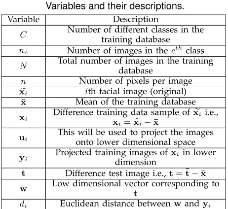
Suppose we have C number of expression classes, let nc be the number of facial images for cth class,
where c ∈ {1, . . . , C} denotes the class index (refer Table 2 for more notations). The total number of facial images can thus be denoted asN =∑Cc=1nc.
TABLE 2
Variables and their descriptions.
Variable Description
C Number of different classes in the
training database
nc Number of images in thecthclass
N Total number of images in the training
database
n Number of pixels per image e
xi ith facial image (original)
¯
x Mean of the training database xi Difference training data sample of e
xi i.e.,
xi=xei−x¯
ui This will be used to project the images
onto lower dimensional space
yi Projected training images of
xiin lower
dimension
t Difference test image i.e.,t=˜t−x¯ w Low dimensional vector corresponding to
t
di Euclidean distance betweenwandyi
into a long vector. Denote xei ∈ Zn×1 as a vector
representation of theith facial image.
Let us start with a training set of facial images e
xi = [xg1,i, . . . ,xgn,i]T ∈ Zn×1, i = 1, . . . , N.
A classifier can be trained using the training data samples to classify an unlabeled test sample. To do this, let us denote the difference training data samples asxi ∈ Rn×1,i= 1, . . . , N where,
xi=˜xi−¯x,∀i, (1)
where¯x= 1 N
∑N
i=1˜xidenotes the mean of the training
data samples.
Let us denote the projected image in the lower dimensional feature space corresponding to the im-age xi = [x1,i, . . . , xn,i]T ∈ Rn×1 as yi =
[y1,i, . . . , ym,i]T ∈Rm×1, wherem≪n. Hence,yi can
be obtained by the following linear projection using the LFDA transformation matrixU:
yi = UTxi, i= 1, . . . , N, (2)
yk,i = uTkxi, k= 1, . . . , m. (3)
In LFDA, the transformation matrixUmaximizes the local-between-class-scatter-matrix SB while
minimiz-ing the local-within-class-scatter-matrix SW:
U= argmax
V
|VTSBV|
|VTS
WV|
, (4)
where,V represents the possible transformation ma-trices i.e., the optimal V which maximizes the argu-ment is equal toU,
SB =
1 2
N
∑
i,j=1
Bi,j(xi−xj)(xi−xj)T, (5)
SW =
1 2
N
∑
i,j=1
Wi,j(xi−xj)(xi−xj)T, (6)
whereBi,jandWi,j are tuning parameters for LFDA.
Interesting readers can refer [25], [29] for more details.
4.2 Classification
In this paper, we consider 1-NN [31]. However, our algorithm can be extended to k-NN and Hamming distance based classifiers since these techniques and 1-NN are mathematically similar.1-NN classifier pre-dicts the matching class of the test image based on the closest training image. Squared Euclidean dis-tance calculation can be used to obtain the disdis-tances between the test image and training images (i.e., in the lower dimension). In order to explain the classification phase, let us denote a test image as ˜t = [te1, . . . ,ten]T ∈ Zn×1 and difference test image
ast = [t1, . . . , tn]T ∈Rn×1, where
t=˜t−¯x. (7)
Denote the low dimensional vector corresponding to tasw = [w1, . . . , wm]T ∈Rm×1 wherem≪n. Now
tis projected by the projection matrix as
w = UTt, (8)
wk = uTkt, k= 1, . . . , m. (9)
The squared Euclidean distance, di, between w and
yi, i= 1, . . . , N is
di= ∥(w−yi)∥22 = ∥(U
Tt−UTx i)∥22,
=
m
∑
k=1
(
uTkttTuk−2uTktukTxi+uTkxixTiuk
)
.(10)
The decision rule of the 1-NN classifier is that the training imagex∗ is said to have same expression of the test image if
d∗=min{d1, . . . , dN}, (11)
whered∗ is smaller than a given threshold T. So far we have discussed the traditional approach in which both the training phase (i.e., feature extraction) and the testing phase (i.e., classification) are carried out by the same party. In the next section, we propose an ef-ficient protocol where the training phase is performed by one-party (i.e., server) whereas the testing phase is collaboratively carried out between two-parties (i.e., between the client and server).
5
P
RIVACY-
PRESERVINGF
ACIALE
XPRES-SION
C
LASSIFICATIONIn this section, we extend the algorithm explained in Section 4 to perform PP FEC. The new algorithm satisfies the following three requirements:
R1: without using highly computationally intensive
public-key homomorphic encryption schemes such as Paillier cryptographic system [16]
R2: hide the client’s input data sample and the
R3: hide the server side classification parameters such
as feature vectors and mean of the database from the client
In order to explain the new algorithm, let us split the testing phase of the traditional approach in Section 4 into four steps as follows:
S1: obtain difference test image i.e., (7)
S2: projecting the difference test image onto lower
dimension i.e., (8)
S3: Euclidean distance calculation i.e., (10)
S4: minimum distance calculation to match the test
image to a known class i.e., (11)
TABLE 3
Variables and their description. We useX(X) to denote if the corresponding variable is known
(unknown) to one party.
Vari-ables
Known only
to the Client Known only to the Server e
xi,¯x,
xi,yi,
ui
X X (see Table 2)
t X (see
Table 2) X
˜ η
X (Noise vector, same dimension as
˜t)
X
η X X (Difference noisevector)
γ
X (differ-ence vector)
X
¯
w X vector corresponding toX (Lower dimensionalη)
¯
di X X (Euclidean distance
between betweenw¯ andyi
mi=
¯
di−di X X
ri X
X (Random integer generated by the server to
hided¯i)
e
di=
¯
di+ri X X
rki,1,
rki,2,
rki,3,
ri,4k
X
X (Random integers generated by the server to
use during the secure two-party computations)
In the following subsections, we explain how each of these steps can be computed without violating the above three requirements (R1–R3). Since our method
preserves the privacy, we add the term “private” to those four steps in order to distinguish our method from the traditional approach. Definitions for the vari-ables used in the following subsections are provided in Table 3.
5.1 Obtain the difference test image in private
Initially, the difference test image needs to be obtained for the classification. However, the client cannot send
the test image,˜t, due to the privacy concerns. Hence, the client only sends noise vector, ˜η ∈ Zn×1, with
same dimension as test image. Since server receives only the noise vector, it cannot get any information about the test image vector. As shown in (7), the server obtain the difference noise vector, ˜η, instead of difference noise vector,η, as follows:
η=η˜−¯x. (12)
However, only the client knows the difference be-tween the test image and the noise image. Let us denote the difference asγ where
γ=η˜−˜t=η−t ∈ Zn×1. (13)
5.2 Projecting the difference noise vector onto the lower dimension space in private
As shown in (8), the server projects the differ-ence noise vector (instead of differdiffer-ence test im-age) and obtains lower dimension vector, w¯ = [ ¯w1,w¯2, . . . ,w¯m] ∈ Rm×1, as follows:
¯
w = UTη, (14)
¯
wk = uTkη, k= 1, . . . , m. (15)
However, using (12), (13),t=˜t−¯x, (9) and (15), we can derivew¯k in terms ofwk,k= 1, . . . , mas follows:
¯
wk = uTk(˜η−¯x) =uTk[(˜t+γ)−x]¯,
= uTk[(˜t−¯x) +γ] =uTk(t+γ),
= wk+uTkγ, k= 1, . . . , m. (16)
The scalar uT
kγ in (16) is unknown to the server.
Hence, the server uses only thew¯k, k= 1, . . . , m
ob-tained in (15) for the distance calculation step instead ofwk, k = 1, . . . , m. We show in Section 5.5 that the
server cannot inferwk from (16).
5.3 Euclidean distance calculation in private
Since the server has only computedw, let us denote¯ the Euclidean distance between w¯ and the low di-mensional training imageyi asd¯i, i= 1, . . . , N.
Sim-ilar to (10), we can compute the Euclidean distances ¯
di, i= 1, . . . , N as
¯
di=∥(¯w−yi)∥22 = ∥(U
Tη−UTx i)∥22,
=
m
∑
k=1
(
uTkηηTuk−2uTkηu T
kxi+uTkxixTiuk
)
.(17)
Since, η=t+γ, we can writed¯i in terms of di, i =
1, . . . , N as
¯
di =
m
∑
k=1
[
uTk(t+γ)(t+γ)Tuk−2uTk(t+γ)u T kxi
+uTkxixTiuk
]
,
= di+ m
∑
k=1
[
uTk (2tγT +γγT−2γxTi)uk
]
[image:7.567.35.274.268.592.2]It is shown in Section 5.5 that the server cannot infer
difrom (18). In the next subsection, we elaborate how
the distances obtained in (18) can be used to obtain the matching training image.
5.4 Minimum distance calculation to match the test image to a known class in private
Let us denote the difference between di
and d¯i in (18) as mi, i = 1, . . . , N (i.e.,
mi =
∑m k=1
[ uT
k(2tγ
T +γγT−2γxT i)uk
] ). Let us rewrite (18) as follows:
¯
di=di+mi, i= 1, . . . , N. (19)
In order to find the minimum distance, the server needs to removemifromd¯i. Since the server does not
know the vectorsγandt, it is infeasible for the server to obtain a true distance valuedifromd¯i, i= 1, . . . , N.
Hence, the server cannot find the matching training image corresponding to the test image using (19). In order to obtain the matching image, the server needs to interact with the client by sending all the
¯
di, i= 1, . . . , N. Before sending d¯i, i= 1, . . . , N, the
server generates random valuerifor eachd¯iand send
e
di to the client where
e
di= ¯di+ri=di+mi+ri, i= 1, . . . , N. (20)
Now the client must interact with the server to com-putemi+ri, i= 1, . . . , N. Usingmi+ri, i= 1, . . . , N,
the client can compute the actual Euclidean distances
di, i= 1, . . . , N as follows:
di=dei−(mi+ri), i= 1, . . . , N, (21)
where
mi+ri= m
∑
k=1
uTk(2tγT +γγT −2γxTi )uk+ri.
Sincet=˜t−x,¯
mi+ri= m
∑
k=1
uTk[2(˜t−¯x)γT +γγT −2γxTi ]uk+ri,
=
m
∑
k=1
uTk(2˜tγT−2¯xγT+γγT −2γxTi)uk+ri,
=
m
∑
k=1
uTk[(2˜t+γ)γT]uk
−
m
∑
k=1
uTk(2¯xγT+ 2γxTi)uk+ri.(22)
It should be noted that mi, i = 1, . . . , N should
only be known to the client. Otherwise, if they are known to the server, then the server can compute the actual Euclidean distances between the test and training images, and eventually the server can obtain the expression corresponding to the test image which violates the client’s privacy. In (22), the vectors˜tandγ
are only known to the client and the vectorsuk,xi,¯x
and the random scalarriare known only to the server.
The vectors and scalars known to the server and client are coupled with each other in (22) and it requires large number of interactions between the client and server to privately computemi+ri. If we reorder (22)
such that, the variables known to the server to be on one side while the variables known to the client to other side then the algorithm in Table 1 can be used to compute (22).
5.4.1 Solve (22) using the Algorithm in Table 1
In order to exploit the algorithm in Table 1, we must rearrange variables in (22). In order to do this, let us now process the first term in (22) (i.e.,∑mk=1u
T k[(2˜t+
γ)γT]u
k) using Kronecker identities as follows:
uTk[(2˜t+γ)γT]uk=vec
{
uTk[(2˜t+γ)γT]uk
}
,
= (uTk ⊗uTk)[γ⊗(2˜t+γ)] = (uTkγ)⊗[uTk(2˜t+γ)],
= (uTkγ)×[ukT(2˜t+γ)]. (23)
Let us assume that the server generates random in-tegers rk
i,1, rki,2, ri,k3, and ri,k4, ∀k to randomize the
scalar product output. If we incorporate these random variables within (23) then (23) becomes equal to (24) (shown in the top of the next page).
In (24), the server knows uk, rki,1, r k i,2, r
k i,3,
and rk
i,4 while the client knows γ and 2˜t + γ.
Hence, the client and server collaboratively compute [
uT kγ+r
k i,1
] ,[uT
k(2˜t+γ) +r k i,2
] , [(rk
i,2uk
)T
γ+rk i,3
] ,
and [(rk i,1uk
)T
(2˜t+γ) +rk i,4
]
using the algorithm in Table 1. In order to balance the equation, the server subtracts (rki,1rki,2−rki,3−rki,4) in (24) in the next computation. Now let us process the remaining terms in (22) (i.e.,−∑mk=1u
T k(2¯xγ
T+ 2γxT
i )uk+ri) as
follows: [second term in (22)-(ri,k1rki,2−rki,3−rki,4)] = −∑m
k=1u T
k(2¯xγT+2γxTi)uk+ri−
(
rk
i,1rki,2−ri,k3−rki,4
)
can be transformed into (25) using Kronecker identi-ties (shown in the top of the next page).
In (25), the server knows
2[(uTk ⊗uTkx) + (u¯ Tkxi⊗uTk)
]
andri+ (rki,1r k i,2−r
k i,3− rk
i,4) and the clients knows γ. Hence, the algorithm
in Table 1 can be exploited by both the client and server in order to compute the [−∑m
k=1u T k(2¯xγ
T +
2γxT
i)uk +ri −
(
rk
i,1ri,k2−rki,3−ri,k4
)
]. Hence, using (24), (25), and Table 1, the client can obtain (mi+ri)
(uTkγ)×
[
uTk(2˜t+γ)
]
+
(
ri,1k r k i,2−r
k i,3−r
k i,4
)
=
[ uTkγ+r
k i,1
]
×[uTk(2˜t+γ)+r k i,2
]
−[(ri,2k uk
)T
γ+ri,3k
]
−[(rki,1uk
)T
(2˜t+γ)+rki,4
]
.
(24)
−uTk(2¯xγ T
+2γxTi)uk+ri−(rki,1r k i,2−r
k i,3−r
k
i,4) = −2vec(u T k¯xγ
T
uk)−2vec(uTkγx T
iuk) +ri−(ri,1k r k i,2−r
k i,3−r
k i,4),
= −2
[
(uTk ⊗u T k¯x)+(u
T
kxi⊗uTk)
]
vec(γ) +ri−(rki,1r k i,2−r
k i,3−r
k
i,4). (25)
5.4.2 Privacy-preserving Expression Finding
Let us define a binary vector db ∈ {0,1}N×1. If nth
Euclidean distance is the smallest distance then, the client generates a binary vector db by setting nth
element to1 while setting all other elements to0. Let us denote the expression ofnth training image asidn
and define another vector called expression vector as dexp= [exp1, exp2 , . . . , expN]T. Client must keep the
binary vector db away from the server in order to
protect the privacy of the test image. However, the client could exploit the algorithm in Table 1 to obtain the expression of the test image without revealing the db as follows: The expression of the training
image which is corresponding to the smallest Euclidean distance (i.e., lets assume nth training image) could be obtained by computing dT
bdexp (i.e.,
[0 0. . .0 1 0 . . . 0].[exp1 . . . , expn, expn+1, . . . , expN]T = expn). It should be noted that the algorithm in Table
1 but with different inputs can be used to obtain the correct expression of the matching training image. If the client feeds the binary vector db instead of aand
if the server feeds the expression vectordexp instead
of s.b and 0 for r to the algorithm in Table 1, then the output of the algorithm should be equivalent to the expression of the matching training image.
5.5 Privacy Analysis
In this section, we analyse whether our algorithm is vulnerable to any privacy leakage. Our algorithm is based on two-party computation and the only possibility that the privacy leakage can happen is during the interaction between two-parties. We use the following O. Goldreich’s privacy definition to proof that our method doesn’t leak any unintended information to client or server:
Privacy definition for the secure two-party computation: A secure two-party protocol should not reveal more information to a semi-honest party than the informa-tion that can be induced by looking at that partys input and output. The formal proof of the definition can be found in [40].
Let us verify whether the proposed two-party com-putation satisfies the privacy definition. As described in Section 5, the proposed algorithm is composed of four sub-algorithms. In the following we show what are the inputs and outputs to and from the client and server, respectively. This will clearly highlight what is already known to client and server. Hence if we
can prove that nothing else can be inferred other than the known input and output with higher posterior probability than prior probability then the proposed algorithm satisfies the privacy definition.
The ultimate aim for client is to keep the test image and the classification result away from the server while the server wants to keep the classification parameters away from the client. Initially (Section 5.1, Section 5.2, and Section 5.3), the client was just sending the noise vector η˜ ∈ Zn×1 to the server
instead the true test image˜t ∈ Zn×1. From these
inputs, the server only know the size of the test image. This is not a privacy leakage since the server knows the size of the images when training the classifier.
In return the server sends the randomized Eu-clidean distances back to the client. As shown in Sec-tion 5.4, the server hides the Euclidean distanced¯i by
random integerriwhere|ri|>|d¯i|in order to achieve
information-theoretic security. The upper bound of |d¯i| for an256×256image is 256×256×(28)2<248,
hence |ri| = 48-bits is sufficiently enough to achieve
the information-theoretic security.
In Section 5.4.1, the client and server interact with each other using the algorithm in Table 1 in order to compute the true Euclidean distances. The clients inputs are γ and (2˜t+γ). As proved in Theorem 2, information-theoretic security can be achieved when the client’s input data is less than 1024-bits. Hence, the server cannot learn any unindented knowledge.
Similarly for the server, if |rk
i,1| > |uTkγ| ∀i, k,
|rk
i,2| > |uTk(2˜t+γ)| ∀i, k, |r k i,3| > |
(
rk i,2uk
)T
γ| ∀i, k, |rk
i,4| > |
(
rk i,1uk
)T
(2˜t+γ)| ∀i, k, and |rk
i,1rki,2−rki,3− rk
i,4| > | −2
[ (uT
k ⊗uTkx)+(u¯ Tkxi⊗uTk)
]
vec(γ), ∀i, k|
then the client cannot learn any additional knowledge from individual scalar products. Below we show that client and sever knows the required size of random number to randomize the inputs.
The client’s inputs areγ and 2˜t+γ where|γ|= 8 -bits and |2˜t+γ| = 10-bits. Since the client’s inputs i.e., |γα| = 88−bits and |(2˜t+γ)α| = 90−bits, are substantially smaller than 1024-bits, the clients data is information-theoretically secure. Since the server knows the size of the clients input data as well as the sizes of the elements inuk, andx¯, the server can
compute the required sizes of the random integersrk i,1, ri,k2,rki,3, andrki,4to information-theoretically secure its parameters. Based on the experiment we obtained that |rk
i,1|= 45>|uTkγ| ∀i, k,|r k
Angry(AN) Disgust(DI) F ear(F E) Happy(HA) N eutral(N E) Sad(SA) Surprise(SU)
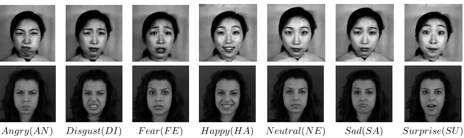
Fig. 1. Example FaE images from JAFFE (1st row) and MUG (2nd row) databases. The 3rd row depicts the expression classes.
|rk
i,3| = 100 > |
(
rk i,2uk
)T
γ| ∀i, k, |rk
i,4| = 100 >
|(rk i,1uk
)T
(2˜t+γ)| ∀i, k, and |rk
i,1rki,2 −ri,k3−rki,4| >
| −2[(uT
k ⊗uTk¯x)+(uTkxi⊗uTk)
]
vec(γ), ∀i, k|.
In Section 5.4.2, the client and server interact with each other using the algorithm in Table 1 in order to identify the matching sample. The size of the client’s input data is1−bit which is smaller than the required 1024−bits of input data, hence the data is information-theoretically secure. Since the server knows the sizes of the client’s input data, it can compute the appro-priate size of random integers in order to protect the expression vector from the client.
At high level, the client’s inputs are element wise randomized before sending them to the server, hence, according to information theory, the client’s inputs are secure. At the end client obtain the Euclidean distance between client’s test image and the server’s training image. However, the client cannot infer any additional information compromise the server’s clas-sification parameters from the Euclidean distance for the following reasons: Euclidean distance is just a positive scalar which was obtained by from feature vectors. From (9) and (10), it is obvious that the scalar value is an aggregated value obtained from large number of variables. Inferring those variables (classification parameters) from a scalar is impossible. Even if the adversary send different inputs, due to the inherent properties of (9) and (10), the outcome will always be a scalar version of previous values.
6
P
ERFORMANCEA
NALYSISThe proposed FEC method was evaluated using two FaE databases: JAFFE [32] and MUG [33]. Fig. 1 shows sample images and expression categories from both the databases. The JAFFE database contains facial images of ten Japanese females, where each has two to four samples for each expression. In total, there are213greyscale FaE images in this database, each of pixel resolution256×256. The MUG database contains image sequences of FaEs belonging to 86 subjects comprising of 35 women and 51 men. Each image
is of resolution 896 × 896. In our experiments we use images of52 subjects, where two to four images were extracted from image sequences per subject per expression, totalling1022images. For the purpose of computational efficiency, all the images were resized to51×51pixels. The number of images used in our experiments and their resolutions are listed in Table 4. In our experiments we convert all the images into 8−bit grayscale images, where each pixel value is8-bit long.
TABLE 4
Details of utilized images from JAFFE and MUG.
Database Subjects Images per Class Resolution
JAFFE 10 28∼32 51×51
MUG 52 110∼120 51×51
In this section we attempt to show that the pro-posed method doesn’t degrade the classification accu-racy due to the randomization. Hence, in this paper, without loss of generality, we use leave-one-out [35] strategy. More precisely, one image is removed from the database and all the remaining images are used for training, while the removed image is used as a test image. This procedure is repeated for a different left out test image each time until all the images are tested. Then we represented the results as a confusion matrix (as shown in Table 5 and Table 7). The accuracy can be inferred in different ways from the confusion matrix i.e., precision, recall, specificity, false positive rate, Matthews correlation coefficient, F1-score and accuracy etc. However the work in [29] uses preci-sion×100 i.e., the ratio between correctly identified expression and total images tested under the same expression times 100. The same strategy applied in this paper too.
The transformation matrix U in (4) can be ob-tained using generalized eigenvectors of matrix pairs {SB,SW}if SW is non-singular. Since the number of
this issue, we exploit the technique used in [23], where PCA transformation matrix WP has been used to
reduce the dimension of the input space such that SWbecomes non-singular in the reduced dimensional
space. Using WP and (4), the LFDA based
transfor-mation matrix WL can be obtained as
WL= argmax
Z
|ZTWTPSBWPZ|
|ZTWT
PSWWPZ|
. (26)
Note that the LFDA transformation matrix U is composed of generalized eigenvectors of matrices of {WT
PSBWP,WTPSWWP}. Now the modified
trans-formation matrix U = WPWL will be used in (2)
and (8) for dimensionality reduction.
In FEC literature, to the best of our knowledge, there is no theory defines how to choose the fea-ture vectors (i.e., how many feafea-ture vectors or which feature vectors) to get optimal classification accuracy. The only way is to do this is based on trial and error. An extensive simulation was conducted in [29] by checking the accuracy against different number of combinations for size of WP and WL. To avoid
repetition and to maintain fair comparison between proposed work and [29], we use the same parameters obtained in [29] for the following experiments.
6.1 Experiments on the JAFFE Database
This subsection describes our series of experiments on the JAFFE database. Initially, we should obtain the dimensions of the WP and the WL corresponding
to best classification accuracy. In order to compare the performance of the proposed method against the Paillier encryption based technique and the conven-tional technique (i.e., without privacy preservation), we exploit the parameter details used in [29]. Denote the dimension ofWP aspand that ofWLasl. Fig. 2
depicts the recognition rates for various values of p
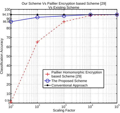
and l. In Fig. 2, top accuracy of 94.37% is achieved whenp= 90and l= 40. Table 5 shows the confusion matrix corresponding to the top recognition rate. Note that for some classes, e.g. the SA class, the recognition rate tends to be lower than other expression classes because the class is highly confused with other ex-pressions [36]. We consider only the top recognition case (i.e.,p= 90andl= 40) to evaluate the proposed scheme. To illustrate the effect of the scalar s in Table 1, we obtained the classification accuracy of the proposed algorithm for five different scalar values and the results were plotted in Fig. 3. In the same figure, we plotted the accuracy of [29] against the scaling factor and the accuracy of conventional scheme ex-plained in Section 4. Our algorithm performs better than [29] for the smaller scaling factors. Also our algorithm achieves the maximum accuracy faster than [29]. This is due to the fact that the work in [29] uses the scaling factor right from the beginning of the classification process (from calculating the difference
50 60
70 80
90 100
110 10
20 30
40 50
89 90 91 92 93 94 95
Dimension of LFDA Transformation Matrix
Dimension of PCA Transformation Matrix
Recognition Rate
[image:11.567.290.530.72.280.2]Top Recognition (94.37%)
Fig. 2. Recognition rate for various dimensions ofWP
andWL for JAFFE database [29].
TABLE 5
Confusion matrix for JAFFE database.
AN DI FE HA NE SA SU Accuracy
AN 29 1 0 0 0 0 0 96.7%
DI 0 27 1 0 0 1 0 93.1%
FE 0 1 30 0 0 0 1 93.8%
HA 0 0 0 29 1 1 0 93.5%
NE 0 0 0 0 30 0 0 100%
SA 0 0 2 1 0 28 0 90.3%
SU 1 1 0 0 0 0 28 93.3%
Average Accuracy 94.37%
test vector). However, our algorithm uses the scaling factor to remove random noise from the Euclidean distances (at the very end of the classification process). This makes our algorithms to reduce the number of errors compared to [29] when the scaling factors are small. The crucial point is that the classification accuracies of both the algorithms eventually become equal to the accuracy of the conventional approach (i.e., 94.37 percent) when s is at a sufficient level, in this case s > 104. Hence, our algorithm doesn’t
[image:11.567.302.512.686.745.2]degrade the classification accuracy due to the privacy preservation.
TABLE 6
Dimensions of PCA and LFDA used to get best performance in MUG database.
101 102 103 104 105 0
10 20 30 40 50 60 70 80 90 100
Scaling Factor
Classification Accuracy
Our Scheme Vs Paillier Encryption based Scheme [29] Vs Existing Scheme
Paillier Homomorphic Encryption based Scheme [29] The Proposed Scheme Conventional Approach
94.37
86.85
[image:12.567.47.240.52.234.2]0.94
Fig. 3. An effect of scaling factor.
6.2 Experiments on the MUG Database
The MUG database contains more facial images than the JAFFE database and includes images of both men and women. Using the MUG database we studied different class sizes against accuracy, scaling factor, dimension of PCA and dimension of LFDA. In partic-ular, we considered three experiments with different class sizes: Exp. 1: 50 images per class, Exp. 2: 81 images per class and Exp 3: 120 images per class. We then empirically obtained the dimensions of PCA and LFDA corresponding to best classification accu-racy. Table 6 shows the details of these parameters. Then experiments similar to the JAFFE database were conducted for MUG database using the proposed method, Paillier encryption based method [29], and conventional scheme. Fig. 4 compares the top classi-fication accuracies for all three methods and for all three class sizes. In Fig. 4, all three methods achieve same accuracy since scaling factor s = 106 has been
used. This is due to the fact that the error caused by integer approximation is compensated by larger scaling factor.
Top recognition rate 95.24% is achieved when the number of images per class is equal to 81 while the performances of other two experiments were below 95%. Hence, the accuracy is not monotonically in-creasing with the class size. From Table 6 and Fig. 4, the dimension of the WP used for dimensionality
reduction increases with that of the class size while the dimension of the WL remains nearly the same
despite increase in class size. The crucial point is that the accuracy of the proposed method is same as the accuracies of existing methods regardless of class sizes. Hence the proposed method doesn’t degrade the performance due to the size of the problem.
In order to evaluate the relation between scaling factor and classification accuracy, we consider the top recognition case. The confusion matrix for the case of 81 facial images per class without privacy
preservation is given in Table 7 when the total number of images, dimensions of PCA, and dimensions of LFDA are 567, 160, and 40, respectively. Then we obtained the accuracies of each expression class by varying the scaling factor using the proposed method. The bar chart in Fig. 5 demonstrates that the num-ber of correctly classified images per class increases monotonically with the scaling factor. The proposed method achieves the results in Table 7 whens= 104. Hence, the proposed method performs equally well as conventional scheme regardless of type of expression class.
350 567 840
92 92.5 93 93.5 94 94.5 95 95.5
% of Correctly Classified Images
Number of Images per Experiment Proposed Scheme
[image:12.567.294.489.219.387.2]Paillier Homomorphic Scheme [29] Conventional Scheme
[image:12.567.287.522.461.576.2]Fig. 4. Comparison of proposed method on MUG.
TABLE 7
Confusion matrix for MUG database in plain domain.
AN DI FE HA NE SA SU Accuracy
AN 78 0 1 0 2 0 0 96.30%
DI 0 76 1 2 0 1 1 93.83%
FE 2 1 72 1 2 0 3 88.89%
HA 1 1 2 77 0 0 0 95.06%
NE 1 1 0 0 79 0 0 97.53%
SA 0 0 0 0 0 80 1 98.77%
SU 1 0 1 0 0 1 78 96.30%
Average Accuracy 95.24%
6.3 Computational and Communication complex-ity
We now compare the complexity of the proposed algorithm against [29]. The recommended key size for Paillier encryption based scheme in [29] is 1024-bits, hence for the sake of comparison, we consider 1024-bits long random integers in the proposed scheme and show that our algorithm still outperforms [29].
6.3.1 Computational complexity
AN DI FE HA NE SA SU 60
65 70 75 80 85
Number of Imgaes Correctly Classified
Classification Accuracy for Different Scaling Factors
s=101 s=102 s=103 s=104 s=105
Fig. 5. Number of images correctly classified in ran-domized domain for each class for different scaling factors.
bits and denote the computational time (in ms) for multiplication, modulo exponentiation in 1024 bits field as Cm and Ce, respectively. Table 8 compares
the complexity of both the schemes for both the server (S) and client (C) (the size of the images, total number of training images, and the total number of feature vectors are denoted as n, N, and m) in terms of the number of modulo exponentiations and multiplications. From [37], we can roughly estimate
Ce≈240Cm. Let us define computational efficiencies
of the proposed algorithm against [29] at the client side and the server side as eC and eS, respectively
where
eC=
Complexity f or client in[29]
Complexity f or client in proposed method,
eS=
Complexity f or server in[29]
[image:13.567.110.514.54.586.2]Complexity f or server in proposed algorithm.
Table 9 shows the computational efficiency of the proposed algorithm for different set of parameters. In Table 9, we calculate the efficiency at both the client and server side by varying the parametersm,N, and n. The computational complexity to the client in the proposed algorithm is almost120 times less than the complexity required for [29]. At the server side, our algorithm outperforms when the total number of training images (N) is less than 300. When N
increases, the efficiency of the proposed algorithm at the server side drops slightly compared to [29] if we don’t consider the parallel computation.
It is obvious from Table 8 and Table 9 that the computation time at the server is dominated by
mN(n+ 1)Cm i.e., Section 5.3 in Table 8. In fact this
computation, as shown in Fig. 6, can be performed in parallel by splitting this intomN X(n+1)Cmi.e.,mN
parallel computations. These computations are
repre-TABLE 8
Comparison of computational cost.
Section for Method in [29] Proposed Method
5.1 C n(Cm+Ce) –
S n(2Cm+Ce) –
5.2 C – –
S m(n−1)Cm+mnCe –
5.3 C N Cm 2nCm
S [(2 + 54mm))CCm+ (1 +
e]N
mN(n+ 1)Cm
5.4 C (2Cm+Ce)log2N N Cm
S (9Cm+ 3Ce)log2N (n+ 1)Cm
Total C
(n+N+ 2log2N)Cm+
(n+log2N)Ce
(2n+
N)Cm
S
[2n+(n−1)m+(2+5m)N+ 9log2N]Cm+ (n+mn+
N+ 4mN+ 3log2N)Ce
(mN+ 1)(n+ 1)Cm
Fig. 6. Parallel Computation at server side.
[image:13.567.290.505.90.585.2]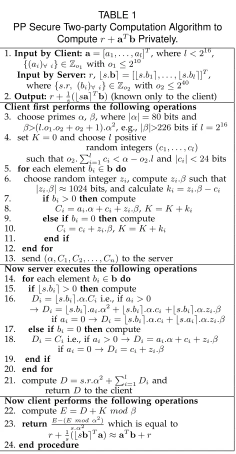
![Fig. 2. Recognition rate for various dimensions of WPand WL for JAFFE database [29].](https://thumb-us.123doks.com/thumbv2/123dok_us/1427239.95370/11.567.290.530.72.280/fig-recognition-rate-various-dimensions-wpand-jaffe-database.webp)