On memories, neural ensembles and mental flexibility

City, University of London Institutional Repository

Citation

:

This is the accepted version of the paper.

This version of the publication may differ from the final published

version.

Permanent repository link:

Link to published version

:

Copyright and reuse:

City Research Online aims to make research

outputs of City, University of London available to a wider audience.

Copyright and Moral Rights remain with the author(s) and/or copyright

holders. URLs from City Research Online may be freely distributed and

linked to.

City Research Online: http://openaccess.city.ac.uk/ [email protected]

1

On memories, neural ensembles and

mental flexibility

Dimitris A. Pinotsis1,2_{, Scott L. Brincat}1 _{and Earl K. Miller}1

1 _{The Picower Institute for Learning & Memory and Department of Brain and Cognitive Sciences}

Massachusetts Institute of Technology, Cambridge, MA 02139, USA

2The Wellcome Trust Centre for Neuroimaging, University College London, WC1N 3BG, UK

Correspondence: Dimitris A. Pinotsis

The Picower Institute for Learning & Memory

and Department of Brain and Cognitive Sciences

Massachusetts Institute of Technology

Cambridge, MA 02139, USA

Tel (+1) 617-252-1790

Fax (+1) 617-452-2588

[email protected]

KEYWORDS: memory engrams; neural ensembles; working memory; neural field theory; auto-encoders; effective connectivity; characteristic path length; betweenness centrality

Acknowledgements. This work is supported by NIMH R37MH087027. DAP gratefully

2 Abstract

Memories are assumed to be represented by groups of co-activated neurons, called neural ensembles. Describing ensembles is a challenge: complexity of the underlying micro-circuitry is immense. Current approaches use a piecemeal fashion, focusing on single neurons and employing local measures like pairwise correlations. We introduce an alternative approach that identifies ensembles and describes the effective connectivity between them in a holistic fashion. It also links the oscillatory frequencies observed in ensembles with the spatial scales at which activity is expressed. Using unsupervised learning, biophysical modeling and graph theory, we analyze multi-electrode LFPs from frontal cortex during a spatial delayed response task. We find distinct ensembles for different cues and more parsimonious connectivity for cues on the horizontal axis, which may explain the oblique effect in psychophysics. Our approach paves the way for biophysical models with learned parameters that can guide future Brain Computer Interface development.

Introduction

3 Previous work has attempted to identify neural ensembles using electrophysiological measures (Brown et al., 1998; Diba and Buzsáki, 2007; Johnson and Redish, 2007) and more recently optogenetics and immediate early gene (IEG) labelling (Ryan et al., 2015). However, due to slow dynamics, these approaches can only provide limited insights into fast activity and neural oscillations that are thought to play a key role in memory function and ensemble formation (Buschman et al., 2012; Fries et al., 2007; Fusi et al., 2016; Haegens et al., 2011; Miller and Buschman, 2013). Thus far, electrophysiology studies have only considered neural ensembles in a piecemeal fashion, that is, using pairwise correlations. They have focused on single neurons and/or functional connectivity between pairs of neurons and/or recording sites; the existence of an ensemble is thus inferred indirectly (Buschman et al., 2012; Gray, 1999; Modi et al., 2014).

Here, we suggest an alternative approach to identifying ensembles based on effective connectivity. We describe ensemble properties using neurophysiological data combined with ideas from biophysical modelling, unsupervised learning and complex systems theory. We analysed multiple-electrode recordings obtained during a classic test of working memory: spatial delayed response (Funahashi et al., 1990; Fuster et al., 1985). We examined LFPs between simultaneously recorded electrodes in dorsolateral prefrontal cortex (PFC), supplementary eye field (SEF), and frontal eye fields (FEF). Our goal was to identify neural ensembles carrying spatial information in a holistic, not piecemeal, fashion and describe the connections that form them.

4 ensemble properties that cannot be observed using pairwise correlations. For example, using topological measures, we found that network connectivity in the spatial delayed response task was different for different cued locations. Cues on the horizontal axis had shorter characteristic path lengths (the least number of steps between different network nodes) than others. This could explain the oblique effect (psychophysics performance is better for stimuli on than off the horizontal/vertical axes). We also found connectivity and corresponding oscillatory dynamics across different spatial scales and different frequencies within cortical areas, which gives a new dimension to cortical network interactions.

Materials and Methods

Experimental Data and Recording Setup

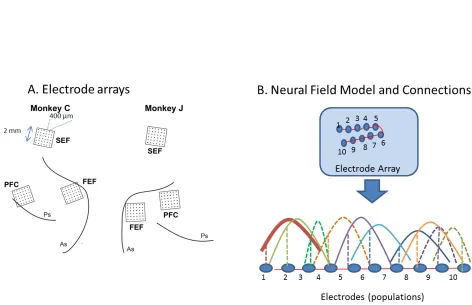
5 area sampled at N_S =32 locations. LFP activity was modelled by a mathematical model of wave dynamics known as a neural field. Electrodes were numbered in a monotonic fashion; neighbouring electrodes had adjacent numbers.

6 Neural ensembles for memory maintenance

Using a neural field model allowed us to use patterns of LFP activity across recording sites to infer the underlying effective connectivity for each of the cued locations. Neural fields provided a quantitative way to describe each ensemble’s network interactions and make predictions about patterns of activity that correspond to different attractor states, see Figure 1B. Each attractor state can be considered to reflect an ensemble or engram (Liu et al., 2012). This is also related to chimera states and metastability (Martens et al., 2016). Our goal was to obtain learned connectivity parameters that can describe the structure of neural ensembles activated while remembering different stimuli. The spacing between electrodes was larger (400um) than what is thought to be the origin of the LFP signal (250um, see Katzner et al., 2009). Using brain decoding algorithms and graph theoretic measures (centrality) we quantified the separability of neural ensembles in SEF and FEF (see below). However, volume conduction could in principle introduce confounds. These can be accommodated by using the effective connectivity parameters obtained here as priors to fit a more complicated biophysical model that accounts for volume conduction effects (Pinotsis et al., 2014). As it is common in computational neuroscience and modern machine learning approaches, we describe neural activity using a one dimensional model. In this model, space is defined along the line traced out by the electrodes. This is similar to ring models (Ben-Yishai et al., 1997; Somers et al., 1995), recurrent neural networks (Botvinick and Plaut, 2006; Sak et al., 2014; Shriki and Yellin, 2016) and deep convolutional neural networks (Krizhevsky et al., 2012). Also, one dimensional neural field models have proven very useful for explaining brain dynamics (Deco et al., 2008; Pinotsis et al., 2013; Robinson et al., 2014).

7 depending on space and time (Jirsa and Haken, 1996; Coombes and Owen, 2004; Breakspear et al., 2006; Breakspear and Jirsa, 2007; Bressloff, 2010; Jirsa et al., 2010; Grindrod and Pinotsis, 2011; Pinotsis et al., 2012a). We here combine neural fields with unsupervised learning to obtain the cortical connectivity underlying interactions at the microscale (within a neural ensemble). This is different from earlier work in the biophysical modeling literature where the connectivity weights are usually chosen ad hoc so that model predictions resemble observed activity, e.g. large scale resting state activity measured with fMRI.

Deep neural fields for memory representations

We assumed that each of the three areas we recorded from (SEF, FEF and PFC) comprised a large number of neural populations (indexed by i=1,..,N,N=32), that was equal to the

number of electrodes we sampled from. These populations were sensitive to different cued locations (values of the visual angleθ). Each of these populations can be thought of as centered around a point υ. They also interact with other populations located at points ψ, via a connectivity function K

(

)

and its state represents cue maintenance.

8 k k

k

Y =

∑

where the constant R will be defined below (see Equation 9) and Gkare the derivatives of

the vector-valued function of perturbations _Xˆ _{of depolarizations}

1( , ) ( , ) ( , ) n x t X t x t υ υ υ     =      

 around

baseline activity X( , )υ t =X0( )υ +Xˆ( , )υ t , with respect to the variable

υ

parameterizes the cortical manifold W occupied by the neural field,

( )

ˆ ( , )

k k X t G υ υ ∂ =

∂ (2)

The functions Gk are the principal axes. zkare the latent variables, which we call the connectivity components. These functions are defined by the following equations

0 1 0 0 1 ! ( ) ( , ) ( ) ( , )( ) W df k

k k W

z df B K d

z B K d

υ ψ υ ψ

υ ψ υ ψ υ ψ

−

− =

= −

∫

∫

Neural fields predict average firing rate or depolarization. To obtain Equation (1), we start from an equation describing the general mathematical form of neural fields

*

X = −BX +K f X +S U (4)

9

(

)

* , , , ( , )

K Q=

∫∫

ψ

rate-constants of postsynaptic filtering.

Equation (4) says that the rate of change of depolarization X of a neural population

occupying a location υ comprises three terms; the first is a simple decay, the second is due to presynaptic inputs from other parts of the cortical manifold and the final part is due to external inputs U, where S:n →n maps exogenous inputs to depolarization. Also,

: n n,

f  → ( ) 1

1 exp( ( ))

f Q

Q

γ η =

+ − is a vector-valued transfer function that describes the

mapping from postsynaptic potentials to average firing rate (Lipschitz continuous to guarantee local existence) of the population around point . Here, γ is synaptic gain and η is the postsynaptic potential at which the half of the maximum firing rate is achieved, see e.g. (Pinotsis et al., 2012b) for more details.

In the literature, the connectivity matrix K

(

)

that isK

(

)

(

)

other studies where there is no invariance constraint, entries of the connectivity matrix are chosen by hand. The novelty of our approach is that we obtained cue-specific entries for this matrix using a Bayesian algorithm. This can be thought of as a probabilistic analogue of the classical principal component analysis (PCA): obtaining the connectivity components amounts to obtaining principal components. This also maximizes the mutual information between the cue and its representation.

Obtaining efficient cue representations using neural fields

A common mathematical simplification in fixed point networks is the assumption of

W

10 stationarity. This eschews the need for explicit numerical integration. It also means that we can drop the explicit time dependence from the equations and functions, e.g. write K

(

)

(

)

1 ( , ) ( , )

X υ t =x υ t following a usual assumption sometimes known as a stable attractor

(Brunel and Wang, 2001). This means that the variable X( , )υ t comprises both excitation

and inhibition. This assumption does not exclude complex dynamics resulting from the interaction of excitatory and inhibitory populations: this was demonstrated by Brunel and Wang who considered mean fields of populations of spiking neurons based on the integrate-and-fire neuronal model. It is the mean field of the population activity that demonstrates the attractor state, which is the level of description chosen here, see also (Pinotsis et al., 2013). Brunel and Wang showed that noise induced in a population of spiking neurons will change the spiking dynamics, but the mean field will have a particular constant value as long as all other characteristics stay the same and this noise is small. These attractor states can be thought of as mediating the flexible formation of neural assemblies associated with different inputs or stimuli. This is not a new idea; attractor states are well known to mediate persistent activity in working memory and similar tasks, see e.g. (Wei et al., 2012). Under the above assumptions, it is straightforward to rewrite Equation (4) in the form of a Taylor expansion

0 0 1 1 2 2

ˆ _...

n n

X ≈z G +z G +z G + +z G (6)

where we linearized fX( , )υ t ≈df X0 ( , )υ t . This result was obtained by expanding with

respect to the space variable υ. In the following, we adopted a probabilistic framework. We assumed that cortical activity Xˆ ( , )υ t ∈X was sampled from a random processX . This

describes activity generated by the cue maintenance. It also means that different trials

ˆ ,l 1,...

X l= S correspond to different realizations of the process X , Xˆl∈X . Adding

Gaussian noise ε with precision 2 2

1 /

s s

11 0 0 1 1 2 2

2

ˆ _...

(0, )

n n s

X z G z G z G z G

s I

ε ε

= + + + + +

 (7)

We then assumed that connectivity components were sampled from a normal distribution

(0, _Q)

zN I . This ensured that they were uncorrelated. We also considered mean-centered

activity

ˆ

1 l

l

Y X m

m X

S

= −

=

∑

We thus obtained Equation (1) where

R= +m ε (9)

We then used a Restricted Maximum-Likelihood (ReML) algorithm to obtain Bayesian optimal values for the connectivity components zk (Harville, 1977). This algorithm optimizes the objective function F

2 2 2 1

1

( ) ( ) ln ln co

2

T T

s s s

F = −_{  }  Y−GZ r Y−GZ + s + s ∆ +− Z Z+ nst_

  (10)

12 2

1 T s

T s I G G Z −G Y

∆ = +

= ∆ (11)

The above expression of the Free Energy obtains from the sum

log ( ) ( ) (0, )

z Q KL Q

F =E_ _ p Y z  −_ D _Q z Y N I _ (12)

under a Laplace assumption, where Q is the approximate posterior and after substituting 2 1

(0, _Q), ( , _s )

zΝ I qQ z Z s ∆− and Y Ν(0,GGT +s I2_{s P}), see also (Friston, 2008). Equation

(12) is the objective function used in variational auto-encoders where the data is generated by a directed graphical model p Y z( ) and the encoder is learning an approximation q to

the posteriorpΝ(z Y).

In summary, we expressed a neural field model as a variational auto-encoder. This allowed us to project high dimensional data (electrophysiological time series) to low dimensional connectivity components z. We call a neural field model with parameters obtained by optimizing a Free Energy cost function, a deep neural field model.

Effective connectivity within a cortical area can be used for cue classification

We used Naı̈ve Bayes and diagonal Linear Discriminant Analysis (LDA) to classify feature vectors comprising connectivity components (Witten et al., 2016). To classify a feature

13

arg max log ( ) log ( )

h p y p z y

θ θ θ

= _ = + = _

 ₍₁₃₎

where h denotes the class (location or angle) and the first and second terms in the brackets are the class prior and the class conditional density respectively. Assuming a Gaussian form for the conditional density,

( ) ( , )

p z y=θ  N µ_θ Σ_θ (14)

results in a decision rule of the form

arg min( ) ( )T log

h z _{θ θ} z _{θ θ}

θ µ µ

= − Σ − + Σ

 ₍₁₅₎

Taking 2 2

1

( ,..., _N)

diag ss ss

θ θ θ

Σ = _{yields Naı̈ve Bayes. Then, the class densities have diagonal}

covariance matrices and the decision rule is the sum of components from each sample vector

(

)

arg min / log

M

l l l l

l

h z _θ ss_θ ss_θ

θ µ

=

∑

 ₍₁₆₎

14

(

)

arg min /

M

l l l

l

h z ss

θ µ

=

∑

 ₍₁₇₎

This is known as diagonal LDA.

Obtaining the connectivity from its components

We assumed a Gaussian connectivity profile for the connectivity K( , )ψ υ

(

)

{

}

2 2

( , ) 2 exp ( ) / 2

K ψ υ C p ψ υ ψ C

−

= − − − (18)

where ψ_and C are the mean and standard deviation. These parameters can be readily obtained using the first three connectivity components A A0, 1 and A2

1

:

1 0

2 0 2 0 1

0 ₀

A A

A A A

A C

A _A

ψ = ℜ

− = ℜ

(19)

This follows standard results in the theory of linear inverse problems (Bertero et al., 1988)

1 ℜ

15 that occur in various branches of physics (Heinz, 2013; Mersmann, 1995). Below, we used a small number of connectivity components to obtain the weights, that isA A0, 1 and A2

2_.

Topological features of neural ensembles

We used the connectivity matrices and graph theoretic measures to describe information flow within neural ensembles, cf. (Sporns, 2013). We first computed the characteristic path length

, 1 / ( 1)

a a b

a b

L N L

≠

= −

∑

We will see below that using this measure allowed us to quantify information transfer efficiency within neural ensembles.

We also used betweenness centrality

\

, ,

1 / ( 1)( 2) ab c

c

a b E ab a b a c

K

X N N

K

∈

≠ ≠

= − −

∑

where Kab c\ is the sum of shortest paths connecting electrodes a and b that do not cross electrode c and Kab is the sum of all shortest paths connecting electrodes a and b. This allowed us to characterize the degree of overlap between different neural ensembles (see below).

2 _{Our approach can be generalised to include different parameterizations for connectivity matrix (e.g.}

16 Results

Identifying neural ensembles

We first used the neural field model to characterise how different cued locations are represented in different cortical areas in a concise and holistic manner, in terms of a few parameters that describe microscale connectivity between recording sites within each area. The parameters that appear in the neural field model describe the dispersion and topography of neuronal connections that are likely to underlie observed patterns of LFPs across recording sites. To obtain them, we trained a neural field model using raw LFP time series and applied a PCA-type algorithm. This process yielded the principal components and axes. Mathematically, the latent variables in a linear model are the principal components. Here, the principal components describe the spatial information in the LFP data. That is, they describe the patterns of activity across recording sites. We focus on the principal components first. In the next section, we will consider another output of the PCA decomposition: the principal axes, which contain the temporal information.

The spatial principal components are matrix-valued functions with dimensionality equal to

T S

N xN , where N_T =600 is the number of trials. We call each entry in these matrix functions the component strength. This expresses the sum of all connectivity weights that target the neurons that contribute to the LFPs observed from each electrode. The connectivity weights are parameters in the neural field model that describe the strength of the effective connections between the recording sites within each cortical area. They describe how the signal is amplified or attenuated when it propagates between recording sites. Large positive weights of connections targeting a certain electrode implies that large LFP responses would be expected from that recording site. These weights are the entries of the connectivity matrix K that multiplies input signal from other electrodes (second term

17 In each panel in Figures 2A-C, we plotted the across-trial averages of the first four connectivity components (blue, orange, yellow and magenta lines, respectively) for all three areas. We will see in the next section that these correspond to the connectivity patterns that are expressed at four different spatial scales. The different panels show connectivity components for the different cued locations. In all these panels, the horizontal axis represents the electrode number and the vertical axis is the strength of the connectivity components.

18

Figure 2. A. Trial average estimates of FEF connectivity components. Connectivity components are matrix-valued functions with dimensionality equal toN xNT S. These describe patterns of activity across recording

sites and the connectivity underlying neural ensembles maintaining different cued locations. Red arrows and blue dashed lines indicate peaks of these components. These correspond to most activated electrodes and define neural ensembles. These ensembles are not due to between-trial variability; they reflect components that are consistently activated for a specific cued location. The value of the cue (angle) is shown in insets on the top left corner of each panel. B.-C. Connectivity components for SEF and PFC respectively. Order of cued locations follows that of Figure 2A.

Red arrows and blue dashed lines indicate peaks of these components that correspond to the recording sites that are most strongly activated: we call these “peak” sites. We suggest that these peak sites describe part of an ensemble for each cued location. Because we took trial-averages of connectivity components, these ensembles are not due to between-trial variability; instead they reflect components that are consistently activated for that cued location.

We then focused on the spatial structure of ensembles and asked whether they showed any traits of topographic clustering. In other words, that cues adjacent in the visual field induce responses that are also adjacent on the cortical surface (Vaina et al., 2014). Our focus was not on optimizing clustering but on preserving the spatial order of recording sites in the connectivity components. This is crucial for comparing and contrasting results from different brain areas3_{. Traits of topographic clustering can be observed by revisiting the}

results of Figure 2. We saw above that large component strengths imply high levels of activation for the corresponding recording sites (peak sites). To test for topographic clustering, we need to consider the connectivity component strengths that correspond not only to peak sites but also their neighbouring sites. To this end, the overall shape of the connectivity components can be quite informative: the FEF and SEF connectivity components have a regular shape that resembles waves (Figure 2A-B), while PFC

3 _{See section Between-area differences in topography and topology of ensemble connectivity below.This also}

19 components have only local (isolated) peaks (they lack the waves, Figure 2C). Considering this together with the fact that large component strengths imply high levels of activation, we concluded that recording sites that are nearby to peak sites will show similar levels of activation as peak sites. This can be seen in the panels of Figure 2 as follows: connectivity component strengths that correspond to sites adjacent to peak sites, are depicted by coloured line segments that lie inside the red circles in panels 2A(i),(iv) and (vi) and 2B(i). Because these segments are smooth and (approximately) horizontal, sites adjacent to peak sites correspond to the same values of the component strength (depicted on the vertical axis) and therefore exhibit the same levels of activation as the peak sites. In other words, a continuous shape of the connectivity component strength implies a continuous activation profile as we move along electrodes placed on the x-axis in the panels of Figure 2. All in all, the regular, wave-like form of the FEF (and to a lesser extent, SEF) connectivity components taken together with the fact that sites that are nearby on the cortex are also adjacent on the horizontal axes of the panels in Figure 2 imply that FEF (and to a lesser extent, SEF) responses will show traits of topographic clustering. This could be explained by the stronger retinotopy in FEF (Funahashi et al., 1989). This can also be seen in the corresponding functional connectivity matrices that show traits of lattice or block structure (Supplemental Figure 1).

To sum so far, we have looked at the organisation of neural activity induced by different cued locations within cortical areas. We used connectivity components to identify neural ensembles associated with these locations. This also allowed us to characterize clustering within the cortical area.

Neural ensembles oscillate at theta, alpha and beta frequencies

20 baseline) whose Lyapunov exponents determine the frequencies observed in sampled LFP activity.

To understand how the principal axes describe these fluctuations consider an analogy with the physical quantities of velocity and acceleration: velocity describes the distance over which a vehicle has moved in unit time. Then acceleration captures changes in velocity in unit time. This means that, for a vehicle moving at an arbitrary velocity, acceleration will vary faster than velocity over time because it is sensitive to changes in velocity. This means that it will operate at a finer temporal scale. Now, one could replace the word “temporal” with “spatial” and think of the second and third principal axes as velocity and acceleration over space instead of time: the first principal axis is a linear approximation to fluctuations around the mean and captures activity changes at the largest spatial scale. Then, the second is sensitive to changes of the first axis at a smaller scale, the third is sensitive to changes of the second at an even smaller scale and so on. Mathematically, they are the partial derivatives of neural activity with respect to the spatial parameter in the neural field model (this parameter describes the location of an electrode). Thus, each principal axis operates at a distinct spatial scale. This also means that the corresponding connectivity component is associated with a certain spatial scale. This follows simply from the usual correspondence between principal axes and principal components in common PCA. Principal axes and connectivity components are thus associated with a hierarchy of spatial scales: each scale being finer than the previous one.

Principal axes revealed characteristic frequencies in the LFP activity induced by a particular cue (similar to the modes of a spring that is perturbed from its original position and then exhibits transient oscillations). Principal axes are matrix-valued functions of dimensionality

T

N xT, where T=720ms is the length of the raw LFP time series. We call each entry in these

21

22

23

Figure 5. Trial averages of PFC principal axes and power spectra following the format of Figure 3. In contrast to the power spectra of figures 3 and 4 that exhibited global theta activity, theta activity in PFC appears to be localised: theta peaks appear only in the spectra of higher order axes and are absent in the spectra of the first axis. Order of cued locations for each panel follows that of Figure 2A.

24 primarily in the theta range: the abscissa of the red dashed line in these panels corresponds to 6Hz. This line corresponds to the peak frequency in the first mode power spectra. This is the power we expect to dominate at large spatial scales because the first mode spectra operate at the largest spatial scale. Also, alpha activity operates at the same scale. In the bottom panels, we plotted the power spectra associated with the second, third and fourth modes for different cue locations. In FEF and SEF, we notice beta rhythms (bottom panels of Figures 3 and 4). Since each higher order mode operates at a finer spatial scale than the previous one, beta rhythms correspond to more localised responses. In PFC spectra, theta peaks appear only in the higher order modes and are absent in the first mode (compare the upper right panel with the bottom panels of Figure 5). This means that theta responses in PFC are more localised than in the other two areas.

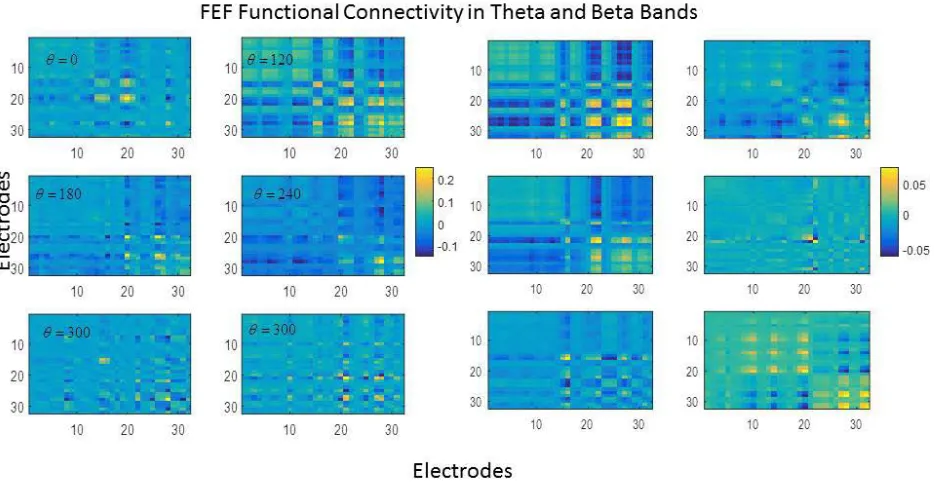
25 are much weaker than in the theta band. Most electrode pairs have strengths around zero with a few electrode pairs with strength 0.05 (orange and yellow) or -0.05(dark blue). There is little synchronised beta activity between electrodes. This result confirmed our earlier conclusion that beta activity corresponds to more localised responses.

Figure 6. FEF Functional Connectivity in the theta (left) and beta (right) bands for different cued locations. Notice the block structure that is reminiscent of retinotopy. Also, functional connectivity values for the beta band are relatively weak. This is because beta oscillations are localised.

Neural ensembles for different cued locations do not overlap

26 neural ensembles that are linked together via sets of connectivity patterns described by connectivity components. However, we have not yet tested the degree to which differences among neural ensembles are expressed by these components. Can we distinguish between memorized cues based on connectivity components? Earlier, we noted that many neurons may participate in multiple ensembles. A large degree of overlap between ensembles might mean that the connectivity components between different recording sites could overlap for different ensembles to the extent that we could not detect any difference in connectivity for the different cues. If, on the other hand, we can, it would help establish this approach as a means for detecting and describing ensembles. Below, we show that we can. This process also allows us to determine whether only a few connectivity components might be sufficient for decoding ensemble activity. From a computational perspective this is important, as having to use too many components would be computationally intractable.

To formally test which and how many connectivity components can sufficiently characterise differences in connectivity for different remembered cues, we used their entries (the 32 connectivity strengths) as classification features of different trials by cued location4_{. Recall}

that each strength expresses the sum of all connection weights that target the neurons that contribute to the LFPs from each of the 32 electrodes.

For our classification analyses, we varied the total number of classification features used by including a different number of connectivity components: the total number of classification features was equal to 32xN_c , where N_c =1,..., 4is the number of connectivity components considered. Letting N_c =1meant that we only used one connectivity component, while

4 c

N = meant that we used all four shown in Figure 2 and so on. The specific goals of this

analysis were: 1. To determine whether we can predict the location of the cue on each trial; 2. To appraise the predictive power (relative accuracy) of each of the connectivity

4

27 components (the curves of different colours shown in the panels of Figure 2) and their combinations. In other words, we wanted to test whether some connectivity components might be more informative than others and whether accuracy would increase when we considered different or more connectivity components for classification (variedNc). We used two different methods for classification, namely Naı̈ve Bayes and diagonal LDA. We used data from 600 trials (450 trials for training and 150 trials for testing. Naı̈ve Bayes and

LDA are among the most commonly used classification algorithms.

28

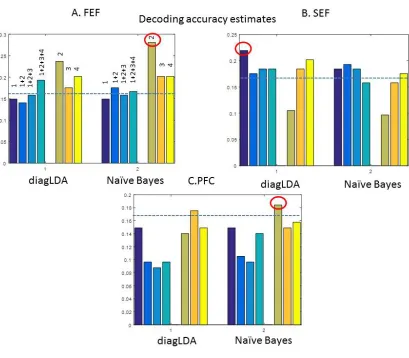
and used Naı̈ve Bayes and diagonal LDA as classification algorithms. Either a single component or multiple components were used (see the numbers above each bar). We obtained significant results for both FEF and SEF. Maximum accuracy in FEF was obtained with the second connectivity component (A), while the first connectivity component yielded maximum accuracy in SEF (B). PFC accuracy estimated appear to be less satisfactory, however the second component resulted in above chance level accuracy (C).

The results of our analysis are shown in Figure 7. The blue dashed line depicts chance level (0.1667). Results obtained using diagonal LDA are shown on the left while accuracy

obtained after applying Naı̈ve Bayes is shown on the right of each panel. Using both methods, we tested whether seven different combinations of connectivity components can be used for classification of the trials by cue location. Either a single component or multiple components were used (see the numbers above each bar, e.g. “1+2” means that we used the first and second components). Overall, both methods gave qualitatively similar results in terms of which features are informative for classification.

We obtained significant results for both FEF and SEF. This revealed which spatial scales of LFP activity are most informative for distinguishing between ensembles corresponding to different cued locations. As we saw in the previous section, each connectivity component corresponds to a spatial scale: the component of highest accuracy corresponds to the most informative spatial scale. In FEF, the second connectivity component (orange curve in the panels of Figure 2A) appears to be most informative (Figure 7A, , cf. the third green-brown bar from the right in the top left panel with the number “2” on top) for distinguishing between various cues maintained in FEF. This means that using a few components is sufficient for describing unique ensemble activity for different cues. It also means that we expect differences in FEF functional connectivity between neural ensembles to be expressed in a fine spatial scale.

29 the greater degree of topographic organisation of FEF responses observed earlier. A higher degree of topographic organisation of FEF in comparison to SEF responses would imply a more organised spatial structure that should be evident at a finer spatial scale.

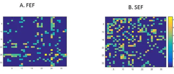
The differences in the most informative components in FEF and SEF described above imply differences in the way LFP electrodes capture information in different frequency bands in the two areas. Functional connectivity was not equally informative in both areas. We found that SEF functional connectivity was informative in more frequency bands than in FEF. It was more sensitive to differences between neural ensembles. We concluded this as follows: We computed pairwise differences in the SEF functional connectivity between neural ensembles in two different frequency ranges: 1. In a narrow range that only included the theta band (cf. Figure 7 left panels) 2. In a broader range that included both theta and alpha bands. We summed together all pairwise differences and obtained two matrices of functional connectivity differences between ensembles: one for the narrow and one for the broad frequency range. We then subtracted these two matrices from each other and thresholded the resulting matrix to focus on the top 50% of the entries5_{. The result is}

shown in the right panel of Figure 8. We also computed the corresponding result for FEF (Figure 8, left panel). We noticed that including the alpha on top of the theta band when computing the functional connectivity in SEF (considering a broader frequency range) enhances the differences between ensembles: the right hand side matrix in Figure 8 includes a larger number of non-zero entries in comparison to the left hand side matrix. This means that a larger number of SEF electrodes were sensitive to differences in functional connectivity between ensembles when we used both theta and alpha bands (to compute the functional connectivity) in comparison to FEF. Thus, a broader range of frequencies is informative for distinguishing between SEF ensembles (in comparison to FEF). This is because SEF activity in the theta and alpha frequency bands is most informative in the largest spatial scale.

5_{Thresholding was done for visualisation purposes and we reached the same conclusion by just considering}

30

Figure 8. Changes in functional connectivity differences between ensembles when changing the frequency range. We computed such differences for a narrow (theta band) range and a broader range that included both theta and alpha bands. We found that a larger number of electrodes were sensitive to changes in the differences in functional connectivity between ensembles when we included the alpha band in SEF in comparison to FEF. Thus, a broader range of frequencies is informative for distinguishing between SEF ensembles.

Although most data features we used yielded results well above chance in both FEF and SEF, the maximum decoding accuracy obtained using FEF data features was higher than when using SEF features: the accuracy achieved for the second FEF connectivity component (0.28) was higher than the accuracy achieved for the first SEF component (0.22), cf. the leftmost bar in the top right panel encircled (Figure7B). The bottom panel in Figure 7 shows the results for PFC. The effects are weaker. However, the second component (orange curve in the panels of Figure 2C) resulted in accuracy above chance level when used for classification with Naı̈ve Bayes; cf. the third bar from the right.

31 components might result in above chance classification accuracy. If so, ensemble activity can be described by a biophysical, neural field model that is computationally tractable. Our results suggest that this is indeed the case: classification accuracy did not dramatically change when we varied the number of components between 1-4: the mean accuracy and its standard deviation after using all possible classification features based on these components and both methods for each area (the mean and standard deviation when we consider all accuracy estimates in the panels of Figure 7) was as follows: 0.162 0.07± for FEF, 0.150 0.06± for SEF and 0.117 0.05± for PFC respectively.

Between-area differences in topography and topology of ensemble connectivity

32 determination η2

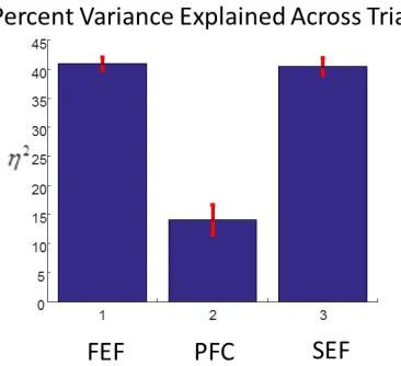
for all regions averaged over all stimuli and trials. This served as a validation of our model and the Gaussian assumption for the connectivity profile. The results are shown in Figure 9 (mean and 90% confidence intervals). Variance explained for both FEF and SEF were around 41%, while PFC showed a lower coefficientη2

, around 14%. This fits comfortably with the traits of topographic clustering in FEF and SEF observed earlier. Had we used a larger number of connectivity components (instead of only three) and determined each of the 1024 strengths independently, we might have got better model performance. However, our current focus was on obtaining a computationally tractable model that involves a small number of parameters. In future work, we will use these parameters as priors to fit Dynamic Causal Models (DCMs), see (Pinotsis et al., 2014, 2015). These models could explain more variance in the data due to the increased number of parameters and description of neurobiological properties of different brain areas.

Figure 9. Percent variance explained after fitting our deep neural field model to data and averaging across all stimuli and trials.

33 by different stimuli or in different tasks in the same or different brain areas. Topology on the other hand, is a notion borrowed from graph theory: Recording sites are thought to occupy the nodes of a graph and to be related to each other through edges that correspond to some pairwise relation measure – usually functional connectivity. Then the topology of cortical activity pertains to non–spatial aspects of relations between responses at different recording sites in terms of graph theoretic measures, like characteristic path length and betweenness centrality (Freeman, 1977). Each site can be connected to any other site in the ensemble in multiple ways that are called paths. One of them is the shortest path. Paths are defined for any pair of sites. Thus each site participates in many shortest paths. Characteristic path length refers to the mean shortest path length between all pairs of sites. Sites that participate in a larger number of shortest paths are more important for the robustness of the neural ensemble. These important sites are also called “central” sites. The term central is reminiscent of graph theory. Betweenness centrality is the ratio of shortest paths in which any given site participates over all shortest path lengths in the ensemble. First, we will discuss the topography of brain activity.

A Gaussian connectivity profile implies that the connection strength between two recording sites is described by two parameters: mean and dispersion. Dispersion is a measure of how extended the corresponding ensemble activity is. The Gaussian connectivity matrices for the three cortical areas and all cued locations are depicted in Supplemental Figure 2. We performed a two-way ANOVA using brain area and cued location (six possible cues) as factor on the mean and dispersion of the connectivity matrices for all areas and possible cues. For each ANOVA we looked at pairwise differences for each possible combination of two brain areas.

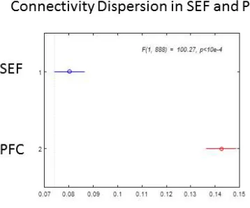
34 = 1.67, p =0.15. Connectivity dispersion in PFC was larger (C = 0.08±0.004) than SEF (C = 0.14±0.004), see Figure 10. A larger dispersion of PFC connectivity in comparison to SEF connectivity also means that PFC activity is more extended on the cortical surface in comparison to SEF activity. This fits nicely with an earlier result in section Neural ensembles oscillate at theta, alpha and beta frequencies above. There we found that power in PFC is concentrated in lower frequencies than in SEF. Had we not known that earlier result, we would have been able to predict it using the result we just found. Given that activity in PFC is more extended than in SEF, and that more extended activity might correspond to more power at lower frequencies (Leopold et al., 2003), it follows immediately that responses in PFC will be more extended than in SEF. This is an illustration of how the neural field model introduced here can link together –seemingly disconnected- spatial and temporal aspects of LFP responses.

Figure 10. Differences in the average values of the mean and dispersion of Gaussian connectivity for SEF vs PFC using two-way ANOVA. Interactions between area and cue factors revealed a significant main effect of area on connectivity dispersion, F(1, 888) = 100.27, p <0 .0001.

35 characterise how efficient information transfer within the network might be. Here, the characteristic path length of an ensemble describes how many processing steps, i.e. steps between recording sites, are required to maintain a cue in memory. Our use of path lengths is similar to their use in functional connectivity studies: instead of correlations, we here consider the effective connectivity weights obtained after training the neural field model as an auto-encoder. All results using graph theoretic measures below exploit the connectivity weight matrices found earlier after taking averages of connectivity components across all trials.

36

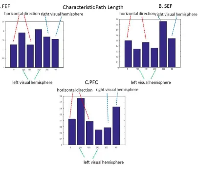
Figure 11. A. Characteristic path length estimates for all FEF ensembles and cued locations. These appear to partition the space of possible cued locations into locations on the horizontal (red dashed lines) and in the left (green dashed lines) and right (blue dashed lines) hemisphere. Also the smallest estimates are obtained for horizontal cued locations; this is reminiscent of the oblique effect. B.-C. Characteristic path length estimates for SEF and PFC. Estimates for both cued locations on the horizontal direction are similar.

We also found that characteristic path length values corresponding to other cued locations (not only the ones on the horizontal direction) also have behavioral relevance. Characteristic path length values appeared to partition the space of possible cued locations into three subsets: locations on the horizontal axis (θ_h =0,180 degrees) and in the left (

120, 240 l

θ = _{degrees) and right (}θ_r =60, 300 degrees), visual hemispheres. They were

37 length corresponding to each of the two cued locations within each of the above three subsets are shown with dashed lines (red for θh, green for θl and blue for θr). Note the similar path length values for cued locations within each subset in FEF. Also note that the characteristic path length values for each pair of locations on the horizontal meridian in all three areas are similar in value.

38

Figure 12. A. Betweenness centrality estimates for all FEF ensembles and cued locations. Neural ensembles do not overlap. Central sites are different for different cued locations. B. SEF betweenness centrality estimates. Similarly to FEF, SEF neural ensembles do not overlap. Notice that SEF central sites are similar to FEF central sites for the same cued location. C. PFC betweenness centrality estimates. Neural ensembles overlap. Central sites are the same for multiple cued locations.

39 with the exception of electrode 15 the rest of the central electrodes correspond to different cued locations in a unique manner. The exception of electrode 15 is not surprising: in the deep neural field model, this electrode is placed in the middle of the cortical manifold, therefore its role as a hub of information flow for the maintenance of more than one cues is expected.

In SEF, we found similar results to FEF: we observed a neural ensemble of electrodes (22-25) on the right end of the figure that exhibits high values of betweenness centrality for

0

θ = _{degrees (}blue dashed lines and ellipses in Figure 12B). Again, we found distinct central electrodes for different cued locations (shown by coloured stars): electrodes 10, 12, 15, 19 and 23 showed peak betweenness centrality values for cued locations at

60,120, 300

40 Discussion

We presented an approach for identifying and describing neural ensembles. Our approach applies ideas from statistical learning in neuroscience (Fiser et al., 2010; Hong et al., 2016, 2016; Jazayeri and Movshon, 2006; Tacchetti et al., 2016; Tsai and Cox, 2015) and is based on a neural field model with learned parameters (Olshausen, 1996; Simoncelli and Olshausen, 2001).

We focused on the connectivity patterns that underlie ensemble responses. The strengths of these connections (connectivity weights) were inferred by analysing LFPs recorded during a spatial working memory task. One motivation for focusing on connectivity weights is recent evidence that working memories are stored in connectivity weights as opposed to neural activity per se (Lundqvist et al., 2011, 2016; Stokes, 2015). The connectivity weights measured the effective connectivity between recording sites. Effective connectivity is a particular sort of functional connectivity where connectivity estimates appear as parameters in a model of observed brain activity. Here, these estimates appear in a neural field model. Traditionally, effective connectivity has been used to describe mesoscale interactions between brain areas using neuroimaging (David et al., 2006; Friston, 1994). To the best of our knowledge this is the first use of effective connectivity to describe microscale interactions underlying neural ensemble dynamics.

To obtain the connectivity weights, we trained a neural field model as a particular type of deep neural network, called an auto-encoder using raw LFP data. Thus, our approach provides links between unsupervised learning literature and biophysical modeling. It is the first illustration of how a neural field model can be used as an auto-encoder network that can learn and maintain its inputs. We call this model a deep neural field. As it is common, we use the term “deep” to describe a neural network architecture with multiple layers, like an auto-encoder. Deep neural fields maximise the mutual information between the remembered cue and the ensemble activity. Therefore, the connectivity weights we obtained are optimal in an information-theoretic sense.

41 micro-circuitry and neuronal interactions. We found that the graph theoretic measures based on effective connectivity at the microscale captured behaviorally relevant information. Characteristic path length estimates in FEF appeared to partition the space of possible cues into those located in the left and right visual field. In addition, the characteristic path lengths were smaller for cues on the horizontal direction, that is, at an angle of 0 or 180 degrees. This means that propagation of information flow within the corresponding neural ensembles occurred faster and engaged shorter paths when storing memories of these cues. The brain seems more efficient on processing stimuli on the horizontal meridian (the oblique effect - Bauer et al., 1979). This in turn might be the result of more parsimonious micro-circuitry.

42 the deep neural field is one-dimensional. All in all, the similarity in the patterns of activity of neural ensembles corresponding to the same stimulus and the way activity is sampled in the two regions could explain the homology between the corresponding central sites.

Finally, we considered oscillatory responses of neural ensembles recorded from different brain areas (Jones, 2016; Schroeder and Lakatos, 2009). Theta rhythms seemed to be prominent in FEF and SEF and were expressed at the largest spatial scale. This is in accord with other studies where theta activity has been shown to be associated with spatial coding both in PFC (Jones and Wilson, 2005) and hippocampus (O’Keefe and Burgess, 2005). We also found beta rhythms. Beta activity has been observed in PFC (Antzoulatos and Miller, 2016; Buschman et al., 2012; Kawasaki and Yamaguchi, 2012; Lundqvist et al., 2016; Stanley et al., 2016). Our approach further revealed connectivity across different spatial scales for theta vs beta frequencies. In FEF, beta was expressed in smaller spatial scales and had weaker functional connectivity than theta. In PFC, power was concentrated in lower frequencies and had larger connectivity dispersion, i.e. extent (spread) of connections compared to SEF. This is consistent with observations that power in lower frequencies is more extended on the cortical surface than power in higher frequencies (Leopold et al., 2003).

43 We considered inhomogeneous connectivity matrices and showed how these can be obtained after training a neural field as an auto-encoder. Our approach yields connection weights that contain information about the particular cue maintained in memory. From a statistical learning perspective, these are learned parameters. From a neurophysiological perspective, they can be thought of as synaptic weights in an animal that has learned to remember the cues. Thus, our approach provides a principled way to obtaining learned connectivity parameters instead of setting them by hand. This paves the way for detailed biophysical models with learned connectivity parameters. Similarly to the deep neural field model introduced here, these models will be able to predict the dynamics of neural ensembles representing different stimuli. They have the potential to explain differences in brain activity associated with stimuli of different values or levels (e.g. cued locations or colours). Importantly, these models could reveal the principles underlying the biophysics and information processing in neural ensembles. These advances could also guide the future development of Brain Computer Interfaces and neuroprosthetics (Nicolelis and Lebedev, 2009).

References

Antzoulatos, E.G., and Miller, E.K. (2016). Synchronous beta rhythms of frontoparietal networks support only behaviorally relevant representations. ELife 5, e17822.

Appelle, S. (1972). Perception and discrimination as a function of stimulus orientation: the" oblique effect" in man and animals. Psychological Bulletin 78, 266.

Atay, F.M., and Hutt, A. (2006). Neural fields with distributed transmission speeds and long-range feedback delays. SIAM Journal on Applied Dynamical Systems 5, 670–698.

Bauer, J.A., Owens, D.A., Thomas, J., and Held, R. (1979). Monkeys show an oblique effect. Perception 8, 247–253.

Beim Graben, P., Pinotsis, D., Saddy, D., and Potthast, R. (2008). Language processing with dynamic fields. Cognitive Neurodynamics 2, 79–88.

44 weakly tuned inputs in a cortical network module. Journal of Computational Neuroscience 4, 57– 77.

Bertero, M., De Mol, C., and Pike, E.R. (1988). Linear inverse problems with discrete data: 11. Stability and regularisation. Inverse Problems 4, 573–594.

Botvinick, M.M., and Plaut, D.C. (2006). Short-term memory for serial order: a recurrent neural network model. Psychological Review 113, 201.

Breakspear, M., and Jirsa, V. (2007). Neuronal dynamics and brain connectivity. Handbook of Brain Connectivity 3–64.

Breakspear, M., Roberts, J.A., Terry, J.R., Rodrigues, S., Mahant, N., and Robinson, P.A. (2006). A unifying explanation of primary generalized seizures through nonlinear brain modeling and bifurcation analysis. Cerebral Cortex 16, 1296–1313.

Bressloff, P.C. (2010). Metastable states and quasicycles in a stochastic Wilson-Cowan model of neuronal population dynamics. Physical Review E 82, 051903.

Brown, E.N., Frank, L.M., Tang, D., Quirk, M.C., and Wilson, M.A. (1998). A statistical paradigm for neural spike train decoding applied to position prediction from ensemble firing patterns of rat hippocampal place cells. The Journal of Neuroscience 18, 7411–7425.

Brunel, N., and Wang, X.-J. (2001). Effects of neuromodulation in a cortical network model of object working memory dominated by recurrent inhibition. Journal of Computational

Neuroscience 11, 63–85.

Buschman, T.J., Denovellis, E.L., Diogo, C., Bullock, D., and Miller, E.K. (2012). Synchronous oscillatory neural ensembles for rules in the prefrontal cortex. Neuron 76, 838–846.

Coombes, S., and Owen, M.R. (2004). Evans functions for integral neural field equations with Heaviside firing rate function. SIAM Journal on Applied Dynamical Systems 3, 574–600.

David, O., Kiebel, S.J., Harrison, L.M., Mattout, J., Kilner, J.M., and Friston, K.J. (2006). Dynamic causal modeling of evoked responses in EEG and MEG. NeuroImage 30, 1255–1272.

De Martino, F., Valente, G., Staeren, N., Ashburner, J., Goebel, R., and Formisano, E. (2008). Combining multivariate voxel selection and support vector machines for mapping and

classification of fMRI spatial patterns. Neuroimage 43, 44–58.

Deco, G., Jirsa, V.K., Robinson, P.A., Breakspear, M., and Friston, K. (2008). The Dynamic Brain: From Spiking Neurons to Neural Masses and Cortical Fields.

Diba, K., and Buzsáki, G. (2007). Forward and reverse hippocampal place-cell sequences during ripples. Nature Neuroscience 10, 1241–1242.

45 Formisano, E., De Martino, F., and Valente, G. (2008). Multivariate analysis of fMRI time series: classification and regression of brain responses using machine learning. Magnetic Resonance Imaging 26, 921–934.

Freeman, L.C. (1977). A set of measures of centrality based on betweenness. Sociometry 35–41.

Freestone, D.R., Aram, P., Dewar, M., Scerri, K., Grayden, D.B., and Kadirkamanathan, V. (2011). A data-driven framework for neural field modeling. NeuroImage 56, 1043–1058.

Fries, P., Nikolić, D., and Singer, W. (2007). The gamma cycle. Trends in Neurosciences 30, 309–316.

Friston, K. (2008). Hierarchical models in the brain. PLoS Comput Biol 4, e1000211.

Friston, K.J. (1994). Functional and effective connectivity in neuroimaging: a synthesis. Human Brain Mapping 2, 56–78.

Funahashi, S., Bruce, C.J., and Goldman-Rakic, P.S. (1990). Visuospatial coding in primate prefrontal neurons revealed by oculomotor paradigms. Journal of Neurophysiology 63, 814–831.

Fusi, S., Miller, E.K., and Rigotti, M. (2016). Why neurons mix: high dimensionality for higher cognition. Current Opinion in Neurobiology 37, 66–74.

Fuster, J.M., Bauer, R.H., and Jervey, J.P. (1985). Functional interactions between inferotemporal and prefrontal cortex in a cognitive task. Brain Research 330, 299–307.

Gray, C.M. (1999). The temporal correlation hypothesis of visual feature integration: still alive and well. Neuron 24, 31–47.

Grindrod, P., and Pinotsis, D.A. (2011). On the spectra of certain integro-differential-delay problems with applications in neurodynamics. Physica D: Nonlinear Phenomena 240, 13–20.

Haegens, S., Nácher, V., Hernández, A., Luna, R., Jensen, O., and Romo, R. (2011). Beta oscillations in the monkey sensorimotor network reflect somatosensory decision making. Proceedings of the National Academy of Sciences 108, 10708–10713.

Hansel, D., and Sompolinsky, H. (1998). 13 Modeling Feature Selectivity in Local Cortical Circuits.

Harville, D.A. (1977). Maximum likelihood approaches to variance component estimation and to related problems. Journal of the American Statistical Association 72, 320–338.

Hebb, D.O. (1949). The organization of behavior: A neuropsychological approach (John Wiley & Sons).

Heinz, S. (2013). Statistical mechanics of turbulent flows (Springer Science & Business Media).

46 622.

Hutt, A. (2013). The anesthetic propofol shifts the frequency of maximum spectral power in EEG during general anesthesia: analytical insights from a linear model.

Jazayeri, M., and Movshon, J.A. (2006). Optimal representation of sensory information by neural populations. Nature Neuroscience 9, 690–696.

Jia, N., Brincat, S., Salazar-Gómez, A., Panko, M., Guenther, F., and Miller, E. (2017). Decoding of intended saccade direction in an oculomotor brain-computer interface. Journal of Neural Engineering.

Jirsa, V.K., and Haken, H. (1996). Field theory of electromagnetic brain activity. Physical Review Letters 77, 960.

Jirsa, V., Sporns, O., Breakspear, M., Deco, G., and McIntosh, A.R. (2010). Towards the virtual brain: network modeling of the intact and the damaged brain. Archives Italiennes de Biologie 148, 189–205.

Johnson, A., and Redish, A.D. (2007). Neural ensembles in CA3 transiently encode paths forward of the animal at a decision point. The Journal of Neuroscience 27, 12176–12189.

Jones, S.R. (2016). When brain rhythms aren’t ‘rhythmic’: implication for their mechanisms and meaning. Current Opinion in Neurobiology 40, 72–80.

Jones, M.W., and Wilson, M.A. (2005). Theta rhythms coordinate hippocampal–prefrontal interactions in a spatial memory task. PLoS Biol 3, e402.

Katzner, S., Nauhaus, I., Benucci, A., Bonin, V., Ringach, D.L., and Carandini, M. (2009). Local origin of field potentials in visual cortex. Neuron 61, 35–41.

Kawasaki, M., and Yamaguchi, Y. (2012). Individual visual working memory capacities and related brain oscillatory activities are modulated by color preferences. Frontiers in Human Neuroscience 6.

Krizhevsky, A., Sutskever, I., and Hinton, G.E. (2012). Imagenet classification with deep convolutional neural networks. In Advances in Neural Information Processing Systems, pp. 1097–1105.

Laing, C.R., and Chow, C.C. (2001). Stationary bumps in networks of spiking neurons. Neural Computation 13, 1473–1494.

Laing, C.R., and Troy, W.C. (2003). PDE methods for nonlocal problems. SIAM Journal of Dynamical Systems 2, 487–516.

47 Leopold, D.A., Murayama, Y., and Logothetis, N.K. (2003). Very slow activity fluctuations in monkey visual cortex: implications for functional brain imaging. Cerebral Cortex 13, 422–433.

Lipinski, J., Sandamirskaya, Y., and Schöner, G. (2009). Swing it to the left, swing it to the right: enacting flexible spatial language using a neurodynamic framework. Cognitive Neurodynamics 3, 373–400.

Lipinski, J., Schneegans, S., Sandamirskaya, Y., Spencer, J.P., and Schöner, G. (2012). A neurobehavioral model of flexible spatial language behaviors. Journal of Experimental Psychology: Learning, Memory, and Cognition 38, 1490.

Liu, X., Ramirez, S., Pang, P.T., Puryear, C.B., Govindarajan, A., Deisseroth, K., and Tonegawa, S. (2012). Optogenetic stimulation of a hippocampal engram activates fear memory recall. Nature 484, 381–385.

Lundqvist, M., Herman, P., and Lansner, A. (2011). Theta and gamma power increases and alpha/beta power decreases with memory load in an attractor network model. Journal of Cognitive Neuroscience 23, 3008–3020.

Lundqvist, M., Rose, J., Herman, P., Brincat, S.L., Buschman, T.J., and Miller, E.K. (2016). Gamma and beta bursts underlie working memory. Neuron 90, 152–164.

Martens, E.A., Panaggio, M.J., and Abrams, D.M. (2016). Basins of attraction for chimera states. New Journal of Physics 18, 022002.

Mersmann, A. (1995). Crystallization technology handbook. Drying Technology 13, 1037–1038.

Miller, E.K., and Buschman, T.J. (2013). Brain rhythms for cognition and consciousness. Neurosciences and the Human Person: New Perspectives on Human Activities 1–11.

Misaki, M., Kim, Y., Bandettini, P.A., and Kriegeskorte, N. (2010). Comparison of multivariate classifiers and response normalizations for pattern-information fMRI. Neuroimage 53, 103–118.

Modi, M.N., Dhawale, A.K., and Bhalla, U.S. (2014). CA1 cell activity sequences emerge after reorganization of network correlation structure during associative learning. Elife 3, e01982.

Neal, R.M., and Hinton, G.E. (1998). A view of the EM algorithm that justifies incremental, sparse, and other variants. In Learning in Graphical Models, (Springer), pp. 355–368.

Nicolelis, M.A., and Lebedev, M.A. (2009). Principles of neural ensemble physiology underlying the operation of brain–machine interfaces. Nature Reviews Neuroscience 10, 530–540.

O’Keefe, J., and Burgess, N. (2005). Dual phase and rate coding in hippocampal place cells: theoretical significance and relationship to entorhinal grid cells. Hippocampus 15, 853–866.

48 Pinotsis, D.A., Moran, R.J., and Friston, K.J. (2012b). Dynamic causal modeling with neural fields. Neuroimage 59, 1261–1274.

Pinotsis, D.A., Hansen, E., Friston, K.J., and Jirsa, V.K. (2013). Anatomical connectivity and the resting state activity of large cortical networks. Neuroimage 65, 127–138.

Pinotsis, D.A., Brunet, N., Bastos, A., Bosman, C.A., Litvak, V., Fries, P., and Friston, K.J. (2014). Contrast gain control and horizontal interactions in V1: a DCM study. Neuroimage 92, 143–155.

Pinotsis, D.A., Leite, M., and Friston, K.J. (2015). On conductance-based neural field models. Frontiers in Computational Neuroscience 7.

Pinto, D.J., and Ermentrout, G.B. (2001). Spatially structured activity in synaptically coupled neuronal networks: I. Traveling fronts and pulses. SIAM Journal on Applied Mathematics 62, 206–225.

Potthast, R., and Graben, P.B. (2009). Inverse problems in neural field theory. SIAM Journal on Applied Dynamical Systems 8, 1405–1433.

Rigotti, M., Barak, O., Warden, M.R., Wang, X.-J., Daw, N.D., Miller, E.K., and Fusi, S. (2013). The importance of mixed selectivity in complex cognitive tasks. Nature 497, 585–590.

Robinson, P.A., Sarkar, S., Pandejee, G.M., and Henderson, J.A. (2014). Determination of effective brain connectivity from functional connectivity with application to resting state connectivities. Physical Review E 90, 012707.

Rubin, J.E., and Troy, W.C. (2004). Sustained spatial patterns of activity in neuronal populations without recurrent excitation. SIAM Journal on Applied Mathematics 64, 1609–1635.

Ryan, T.J., Roy, D.S., Pignatelli, M., Arons, A., and Tonegawa, S. (2015). Engram cells retain memory under retrograde amnesia. Science 348, 1007–1013.

Sak, H., Senior, A., and Beaufays, F. (2014). Long short-term memory recurrent neural network architectures for large scale acoustic modeling. In Fifteenth Annual Conference of the

International Speech Communication Association, p.

Schroeder, C.E., and Lakatos, P. (2009). Low-frequency neuronal oscillations as instruments of sensory selection. Trends in Neurosciences 32, 9–18.

Shriki, O., and Yellin, D. (2016). Optimal Information Representation and Criticality in an Adaptive Sensory Recurrent Neuronal Network. PLoS Comput Biol 12, e1004698.

Somers, D.C., Nelson, S.B., and Sur, M. (1995). An emergent model of orientation selectivity in cat visual cortical simple cells. The Journal of Neuroscience 15, 5448–5465.