A new algorithm of SAR image target recognition based on improved deep convolutional neural network

(will be inserted by the editor)

A New Algorithm of SAR Image Target Recognition based on Improved

Deep Convolutional Neural Network

Fei Gao1 _{· Teng Huang}1∗ _{· Jinping Sun}1∗ _·

Jun Wang1 · Amir Hussain2 · Erfu Yang3

Received: date / Accepted: date

Abstract Background:To effectively make use of deep learning technology automatic feature extraction ability, and enhance the ability of depth learning method to learn and recognize features, this paper proposed a deep learn-ing algorithm combinlearn-ing Deep Convolutional Neural Network (DCNN) trained with an improved cost function and Support Vector Machine (SVM).

Methods:The class separation information, which explicitly facilitates intra-class compactness and inter-class separability in the process of learning features, is added to an improved cost function as a regularization term to enhance the feature extraction ability of DCNN. Then the improved DCNN is applied to learn the features of SAR images. Finally, SVM is utilized to map the features into output labels.

Results:Experiments are performed on SAR image data in Moving and Stationary Target Acquisition and Recognition (MSTAR) database. The experiment results prove the effectiveness of our method, achieving an average accuracy of 99% on ten types of targets, some variants, and some articulated targets.

Conclusion:It proves that our method is effective and CNN enjoys a certain potential to be applied in SAR image target recognition.

Keywords synthetic aperture radar (SAR) images·automatic target recognition (ATR)·deep convolutional neural Network (DCNN)·support vector machine (SVM)·class separation information

1 Introduction

Synthetic Aperture Radar (SAR) possesses all-time and all-weather imaging capability even in harsh environ-ments. As an important means of earth observation currently, it has been widely used in both military and civil fields. Automatic Target Recognition technology of SAR images (SAR-ATR), which can effectively obtain the target information and improve the ability of automatic information processing, has become one of the research hotspots.

SAR-ATR systems generally consist of three stages: detection [1, 2], recognition, and classification. At present, common methods of SAR-ATR include template matching [3], support vector machine (SVM)[4], Linear interpolation [5] Principal Component Analysis [6,7], multi-modal dictionary learning and sparse representation combined [8,9], etc. These methods have been successful in some way, but they rely heavily on experience of ex-perts. The SAR image is vulnerable to various environmental factors, e.g., speckle noise and background clutter, leading to difficulties in the feature extraction of interested targets. In addition, shift sensitivity and pose sensitiv-ity also cause instabilsensitiv-ity in SAR targeting. Therefore, these methods have a certain blindness and unpredictabilsensitiv-ity when applied to SAR images.

Recently, Deep Learning has been an increasingly hot topic in the field of pattern recognition, and experi-mental achievements have been emerging. In 2006, Hinton et al. [10] proposed an unsupervised greedily method based on Deep Belief Network (DBN), which trained deep networks layer by layer, solving the vanishing gra-dient problem. It also made the number of neural networks in a deeper direction with the help of GPU. After

∗_{Corresponding Author, E-mail: [email protected], [email protected], Tel.: 010-82317240,Fax: 010-8231724}

1_{School of Electronic and Information Engineering, Beihang University, Beijing 100191, China}

2_{Cognitive Signal-Image and Control Processing Research Laboratory, School of Natural Sciences, University of Stirling, Stirling}

FK9 4LA, UK

3_{Space Mechatronic Systems Technology Laboratory, Department of Design, Manufacture and Engineering Management, University}

that, many scholars proposed various deep learning models under different application backgrounds, such as the Deep Restricted Boltzmann (DRB)[11], Deep Belief Network (DBN) [12,13], Stacked Auto Encoders (SAE) [14] and Deep Convolutional Neural Network (DCNN) [15]. Among them, some models based on DCNN have made breakthroughs endlessly in both theory and practice of image target recognition. For example, the AlexNet model, which won the championship in the contest of ImageNet ILSVRC in 2012, was recognized as the standard model of DCNN. The top-5 error rate of the AlexNet model was only 16%, 10% lower than the last champion algorithm. The Residual Neural Network [16] won the championship in the same contest in 2015 and obtained only 3.75% error rate, which even outperformed human eyes. DCNN can not only automatically extract target features without too much experience of experts, but also deal with the two-dimensional image data directly. It means the features extracted by convolution kernel are irrelevant to the shift, scaling, and rotation of targets in images [17,18]. This characteristic of DCNN provide a new idea to solve shift sensitivity, and pose sensitivity problems of SAR targets in automatic feature extraction.

Nowadays, the DCNN-based SAR-ATR system is being gradually proposed. To auto-learn features of SAR images rapidly, general methods start with the framework of AlexNet model. The promotion of training efficiency and recognition accuracy are achieved by optimizing a certain model. For instance, Chen et al. [19] initialize the hyper-parameters of DCNN with an unsupervised sparse auto encoder machine rather than the Back Propagation algorithm used in AlexNet model. The unsupervised sparse auto-encoder machine possesses the auto-learning capacity, which accelerates the feature learning of DCNN. The experiment of this method [19] on Moving and Stationary Target Acquisition and Recognition (MSTAR) database obtains a target recognition accuracy of 90.1% for 3 classes and 84.7% for 10 classes. Similarly, Li et al. [20] used the auto-encoder machine to initialize the DCNN. The difference is that fully connected layers work as a final classifier in [20], which greatly reduces train-ing time of DCNN on the premise of ensurtrain-ing accuracy. Although the accuracy of two methods is not very high, there is less dependence on experience of experts in the process of feature learning. Some scholars [21] apply DCNN to automatic feature learning as well, whereas the final output layer becomes a SVM classifier rather than a fully connected layer, constituting DCNN+SVM model. The model makes full use of the DCNNs superiorities in auto-learning of various features and the strong generalization ability of SVM, avoiding weak representation ability of SVM on high-dimensional samples [22] and poor stability of DCNN. With this framework, the classifi-cation accuracy of the method reaches 98.6% [21]. Because of these advantages of DCNN+SVM, such methods have been rapidly developed. On the basis of the work in [21], Wangner et al. [23] introduce Morphological Component Analysis to preprocess SAR image. It rejects some abnormal testing samples so that the accuracy reaches 99% and the recall comes up to 97.3%.

Furthermore, shift sensitivity or pose sensitivity of targets can be solved by Data Augmentation technic, which adds speckle on training samples or extend training samples by shifting and rotating targets. For example, the SAR targets are rotated in [21] to acquire augmented training samples. Ding et al. [24] extend the MSTAR training samples by shifting, attitude synthesis, and adding speckles, achieving a higher accuracy on the standard DCNN methods. Chen et al. [25] augments training samples by shifting, and obtained a 99% classification accuracy using All-convolutional networks. A higher accuracy is acquired in [26] which extends classifier by displacement- and rotation-insensitive, and it is robust to shift and rotation. Whats more, Data Augmentation technic can suppress overfitting and advance recognition accuracy.

In summary, the SAR-ATR system based on DCNN has achieved varying degrees of success, but it is still in its in-fancy. The research is generally conducted from the perspectives of the exostructure architecture of DCNN or the Data Augmentation, yet little focus on the optimization of internal functions in DCNN. The CNN+SVM model proposed in [21], for instance, uses the quadratic function as error cost function. Although the classification accuracy is satisfactory, it would be time-consuming if the neurons make an obvious mistake during the training of DCNN [18]. Compared with error cost function, the Cross-Entropy is applied as the loss function in [24,25,27], while there is a lack of in-depth optimization. In order to improve the classification ability of CNN, we attempt to add class separability information to cross-entropy cost function as a regularization term in DCNN+SVM model. The remainder of this paper is organized as follows. Section II gives an introduction of the basic principle of DCNN for a better understanding of our DCNN+SVM. Section III describes our DCNN+SVM in detail. Experimental results on the MSTAR database are presented in Section IV. Section V concludes our work.

2 Deep Convolutional Neural Network

The mapping in DCNN is a forward propagation process which describes the ”flow of information” through the whole neural network from its input layer to its output layer, so the output of the upper layer is actually the input of the current layer. To avoid the defects of linear model, neurons of each layer need to be added with a nonlinear activation function in the forward process. Since the first layer only receives pixel values from the image, there are no activation functions. The nonlinear activation functions are employed from the second layer and the output of thelthlayer can be expressed as:

zl_=Wl_∗xl−1_+bl

al=σ(zl)

(1)

wherelrepresents thelthlayer, and∗means convolution operation. Whenl=2,x2−1=x1is the image matrix whose elements are pixel values, and whenl>2 ,xl−1is the feature map matrix extracted from the(l−2)th_layer i.e.,xl−1=al−1=σ(zl−2).Wl,bl, andzl are weight matrix , bias matrix, and weighted input of thelthlayer, respectively, andσ is nonlinear activation function. SupposingLis the output layer,aLwill represent the final

actual output vector.

The Back Propagation (BP) algorithm [28], which is a supervised learning method, is commonly used to iteratively update parameters ofWlandbl. It first applies the actual output and the targeted values to construct a cost function, and then applies the Gradient Descent (GD) along the negative gradient direction of cost function to adjust and parameters. The specific process is as follows:

Cost function selection.Normally the quadratic function is selected to be error cost function. However, it would be time-consuming if the neurons make an obvious mistake during the training of DCNN [18]. Thus we take Cross Entropy (E0L) rather than quadratic function as error cost function. According to the forward

propagation algorithm (the equation (2)), the Cross Entropy can be inferred:

E0L=

1 n n

∑

∑

[t_kLlnaL_k+ (1−t_kL)ln(1−aL_k)] (2)

wherenis the total number of training set, andNis the number of neurons in output layer, which means DCNN is finally divided intoNclasses.t_kLis the targeted value corresponding to thekthneuron of output layer, andaL_kis the actual output value of thekthneuron of output layer.

Calculation of error vectors.The error vector of each layer is defined and the error vector corresponding to thekth_{neuron of output layer is expressed as:}

δL=∂E

L

0

∂zl (3)

In BP process,δLcan be used to reversely deduceδL−1 . Similarly, supposeδlandδ(l+1)are the error vectors

of thelthand(l+1)th_{layers respectively. Then according to (1), (3), and the Chain Rule,}

δlis written as:

δl=Wl+1δl+1σ

0

(zl) (4)

where the symbolicis Hadamard product (or Schur product) which denotes the elementwise product of the two vectors.

Updates of weights.The gradients ofWlandblare ∂E L

0 ∂Wl and

∂E₀L

∂bl respectively. The symbolic∂(·)represents partial derivative operation. The partial derivative ofE₀LtoWlandblcan be calculated according to (1) and (3):

∂EL

0 ∂Wl =

∂EL

0 ∂al

∂al ∂Wl =δ

l_xl−1

∂EL

0 ∂bl =

∂EL

0 ∂al

∂al ∂bl =δ

l







(5)

The updated values ofWl andblare represented with∆Wland∆bl, and they are calculated by minimizing the cost function respectively:

∆Wl=−η∂E0l ∂Wl

∆bl=−η∂E

l

0 ∂bl







(6)

3 Improvement of Deep Convolutional Neural Network

3.1 The introduction of class separability information

To enhance the class separability of the features extracted by DCNN model, the class separability information is added to cross-entropy cost function as a regularization term to train DCNN. The class separability information consists of intra-class compactness and inter-class separability, which are expressed asE1andE2respectively:

E1=

1 2

∑

n

c−Mck22 (7)

E2=

1 2 B

∑

Mc−M_c0

2

2 (8)

whereyn_cdenotes the actual output value of thenthtraining sample which belongs to thenthclass.McandM_c0 are the output average values of the training samples incth_and(c0₎th_{classes.Bis the number of training samples} in(c0)th_classes.E

1andE2respectively denote the intra-class distance and the inter-class distance of the output

features. Shortening the intra-class distance and increasing the inter-class distance in every iteration are necessary to enhance the separability of the output features. It is added in the cost function as a regularization term and the modified cost function is as follows:

E=E0L+αE1−βE2 (9)

whereαandβare both weight parameters.

The purpose of modifying the cost function is to adjustWl andbl to make the network develop in favor of classification, and the error vector of modified cost function is essential.

The error vector ofE1in the output layer is:

δ1L=∂_∂E_zL1

= ∂ ∂zL

1 2ky

n c−Mck22 = (1− 1

nc)σ 0

(zL)(yn_c−Mc)

(10)

wherenc_{is the number of samples that belong to the classc.} The error vector ofE2in the output layerLis:

δ2L=∂E2

∂zL

= ∂ ∂zL

1 2

Mc−M_c0

2 2 =_n1cσ

0

(zL)∑B

c0

(Mc−M_c0)

(11)

According to (3), (9), (10), and (11), the new error vector ofEin the output layerLis:

δ0=δL+α δ1L−β δ2L

=σ0(zL)(yn−tn) +α(1− 1

nc)σ 0

(zL)(ycn−Mc)

−β_n1cσ 0

(zL₎B

∑

c0

(Mc−M_c0)

(12)

After getting the error vector in the output layer, we can calculate the error vector in each layer iteratively by using (4). The updated parameters ofWlandblfor each layer can be derived by (5) and (6) afterwards.

3.2 Application of Support Vector Machines (SVM)

3.3 Modified Model

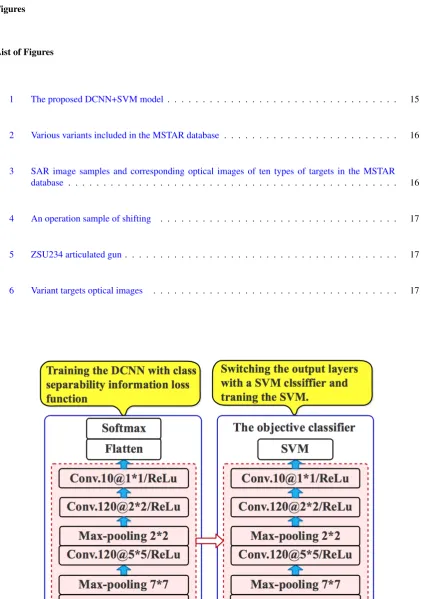
A novel DCNN+SVM model of SAR image target recognition is proposed based on above analysis. Firstly, DCNN is trained combining with the Softmax classifier, where the Cross-Entropy added with the class separabil-ity information is used as the cost function. After training the DCNN, Softmax is removed and the top features of DCNN is utilized to train SVM. Finally, the proposed framework DCNN+SVM is constructed, where DCNN is used to extract sample features and SVM is used as the classifier, as is shown in Figure1.

4 Experiment

4.1 Experiment data

In order to verify the validity of the proposed method, this paper uses the data from the MSTAR database, co-funded by National Defense Research Planning Bureau (DARPA) and the U.S. Air Force Research Laboratory (AFRL). As a benchmark data set, MSTAR is widely applied for development, test, and evaluation of advanced ATR systems [29]. Therefore, adopting the MSTAR data is convenient for comparison with peer algorithms.

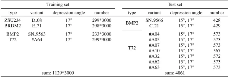
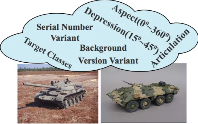
The MSTAR database includes different types of targets and their various serial numbers variant (vehicles that are of the same class and version, but are different serial numbers), version variant (differences from the manufacturer, target of same class but were built to different blueprint), articulation, aspect angles and depression angles. Figure2shows detailed parameters of MSTAR database. The size of each target chip is 128∗128, and the resolution is 0.3 m∗0.3 m. The aspect angle covers from 0◦ to 360◦, and the interval is 1◦ to 5◦, which means there is one SAR image for every 1◦to 5◦. This paper applies ten types of targets: 2S1, ZSU234, BMP2, BRDM2, BTR60, BTR70, D7, ZIL131, T62, and T72. As for their high-level classifications, 2S1 and ZSU234 are artillery; BMP2, BRDM2, BTR60, BTR70, D7, and ZIL131 are assigned to truck; T62 and T72 belong to tank. Their SAR image samples and corresponding optical images are shown in Figure3. The experiment is performed on the above ten types of targets, some other variants, and some articulated targets.

In order to explain our method more clearly and evaluate the performance of our method in a comprehensive way, the experiment is carried out under standard operating conditions (SOC) and extended operating conditions (EOC). The SOC means that the testing conditions and the training conditions are very similar [29], for example, 10 types of targets under 17◦depression are taken as the training samples while the ones under 15◦depression are used as testing samples. However, the EOC means that there are huge dissimilarities between the training set and the testing set [29], such as the significantly different depression angles, different variants of the same target, etc. The Correct Class Probability (Pcc) is applied as the evaluation index of these experiments, and its expression is as follows [30]:

Pcc=

ncc

ntt

(13)

Wherenccis the number of targets classified correctly,nttis the total number of tested targets. In general,Pccis often presented combining with the confusion matrix.

4.2 Experiments under SOC

A This experiment aims to classify ten types of targets under SOC. The ten types of vehicle target chips at 17◦ and 15◦depression angles mentioned in Section4.1are used as a training set and testing set respectively. The detailed information of type, size, and amount is shown in Table1. In order to reduce the input dimension, 64∗64 pixels in the central part of the chip is intercepted as the input sample under the premise that the complete target still locates at the central position. With above data, this experiment is divided into two groups. One only uses the original data as train dataset, while another extends train dataset by Data Augmentation. The DCNN+SVM model in [19] and the DCNN+Softmax model in [27] are used as the contrast method.

The parameters of our model in this paper are set as follows. This model includes the input layer, the output layer, 4 convolutional layers and 2 pooling layers. Generally, a convolutional layer and a pooling layer are together regarded as a convolutional layer, so there are 6 layers in total. The first convolutional layerConv(other layers follow the labeling rule) contains 18 neurons, and the size of convolution kernel and pool are set to 9∗9 and 7∗

ReLu is used as the activation function, and the initial bias and the learning rate are set to 0 and 1 respectively. The initial weight value of each layer is generated randomly in following interval:

"

−4

s

6

f anin+f anout ,4

s

6

f anin+f anout #

(14)

wheref an_inis the number of input feature map of each layer. f an_outis the number of output feature map of each layer. Other parameters,αandβin (9), are set toα=0.03 andβ=2.

4.2.1 SOC 1:The data in Table1is used, where there is no extended data.

The experimental results of the proposed method are shown in Table2. Table3 gives the results of contrast method, which applies the standardized quadratic cost function in the training process combining with Softmax and uses Softmax as a final classifier [19] (here only recapitulating its sequence). The average accuracy of our method is 97.84%, 13.14% higher than that of DCNN+Softamx. As for inter-class error, we find from Table2that only one truck is wrongly classified into tanks. The intra-class confusion in Table2is overall satisfactory, with no confusions in tanks, only one in artilleries, and slightly more in trucks. The confusions of BTR70 and BTR60 are relatively more, which may be caused because BTR70 is an upgraded version of BTR60. For DCNN+Softmax model, however, there are serious confusions in both inter and intra classifications. It proves that adding the class separability information to Cross Entropy error cost function is conducive for distinguishing the high-level classes.

4.2.2 SOC 2:The data in this experiment is augmented by rotating and randomly shifting.

Shifting:The number of extended samples of each chip can be increased up to(128−64+1)∗(128−64+1) =

4225 by shifting in case that every sample contains a complete target. An operation sample is shown in Figure4.

Rotating:We apply the method in [26] to extend training samples, which rotates each chip every 24 degrees. Thus 15 extended chips are generated for each chip.

Combining the rotation and the random shift operation, each chip can be expanded to 4225∗15 chips at most. We select 3000 chips for each type of vehicle targets from the extended dataset. Then the same operation as experiment SOC 1 is carried out on the extended data. Table4shows the experimental results of the proposed method. The average accuracy in Table4reaches 99.15%, better than that in Table2. There is no error in high-level classification, and confusion only appears in trucks for intra-class classification. Compared with the results of experiment SOC 1, the intra-class confusion in trucks reduces a lot in this experiment, and the accuracy is further enhanced as well.

As is introduced in the introduction section, the classification model in [21] is very similar with ours. The distinction lies in that we adopt the Cross-Entropy added with class separability information as the cost function rather than quadratic function. Since the experimental results in [21] do not include detailed information of ten types of targets, we only care about the average accuracy. Their average accuracy is 98.6%, 0.55% lower than ours. The DCNN+Softmax model in [27] employs Cross Entropy as cost function, and its experimental results are given in Table5. Compared with Table4, we find that there are more errors between high-level classes and more confusions between intra classes in Table5. It proves that our cost function increases the class separability to some extent, especially for high-level classes.

4.3 Experiments under EOC

In this section, the experiment is performed under Extended Operating Condition (EOC), which is crucial to determine whether the ATR algorithm can be applied on the battlefield. To verify the reliability, stability, and the generalization ability of our method, we divide the experiment into 4 groups according to various experimental data in Figure2. It is noted that each training samples of EOC series experiment is expanded to 3000 by the method described in section4.2.2.

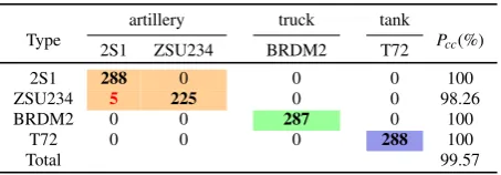
4.3.1 EOC 1: The depression angles of the training set and the testing set are significantly different.

We select 2S1 (B 01), BRDM2 (E 71), T72 (#A64), and ZSU234 (D 08) four types of vehicle targets in this experiment, where the depression angles for the training set and testing set are 17◦and 30◦respectively. Table6

an accuracy of 99.57% is achieved, whats more, no error appears in high-level classes and only 5 confusions exist in the intra-class of artilleries. Thus we can conclude that our method works stably though the gaps of depression angles between the training set and testing set are large.

4.3.2 EOC 2: Some articulated targets are contained in the testing set.

Articulation means some parts of a vehicle change from one state to another, such as a newly added fuel tank or a barrel in different direction [31]. An articulated sample of ZSU234 is shown in Figure5. It is essential to perform this experiment for articulated targets commonly appear in battlefield. To better simulate the practical conditions, we add some articulated targets into the training set and testing set, meanwhile, we keep 17◦ and 30◦ for the training set and testing set. For each high-level class, we select only one type of target in this experiment, and the detailed experimental data is given in Table8. Table9shows the experiment results, and we find the accuracy of each class reaches 100%. Therefore, our method behaves well when articulated targets are included in testing samples.

4.3.3 EOC 3: The testing set contains one type of vehicle and its version variants, and the depression angle is not single.

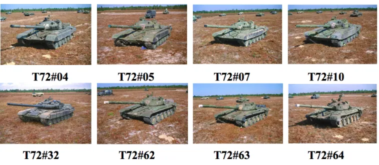
BMP2, BRDM2, one type of version variants of T72 (#64), and ZSU234 consist of a training set, while the testing set only contains T72 and its version variants ( #A04, #A05, #A07, #A10, #A32). The version variants belong to the same class, but the manufacturers are different, and the blue prints of manufacturing are different as well [30]. The variants mentioned above are shown in Figure6. The depression angle of the training set is 17◦, while the testing set has a 15◦depression angle apart from 17◦. Table10shows the detailed data information. From Table11, we find that testing accuracy is up to 100%, so the version variants of T72 cannot impact high-level classification.

4.3.4 EOC 4: The testing set contains multi types of vehicles and their variants, and the depression angle is not single.

The training set is the same as (4.3.3) under EOC 3, while the testing set contains two types of version variants of T72 (#A62, #A63) and two types of serial number variants of BMP2 (SN 9566, C 21). The detailed data is shown in Table12, and the experimental results are given in Table12. The accuracy reaches 99.82%, and there is a small number of confusions only in the trucks. Hence the version variants of T72 will not impact high-level classification, and the impact of serial number variants is also very little.

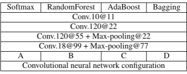
4.4 Comparison with other algorithms

In order to compare with the performance of other algorithms, this paper conducts the comparison from two aspects. One is the comparison with the algorithms in recent published papers, the other is the comparison with some ”CNN+ Classifier” models.

Table14 shows the comparison sheet of classification accuracy of recent published papers. The involved algorithms include Extend Maximum Average Correlation Height (EMACH) [32], Iterative Graph Thickening (IGT) [33], Sparse Representation of Monogenic Signal(MSRC) [34], Monogenic, Scale Space (MSS) [35] and Modified Polar Mapping Classifier (M-PMC)[36]. From Table14, we find the accuracy of the proposed method in this paper is higher than other algorithms.

5 Conclusion

Aiming at the issue of SAR image target recognition, this paper presents a novel method of SAR image target recognition based on CNN. The CNN is improved by adding the class separability information into Cross Entropy cost function and applying support vector machine (SVM) instead of Softmax classifier. The experimental results show that the proposed method achieves a recognition accuracy of 99.15% for ten types of targets with extended training data. In other experiments under EOC, the average recognition accuracy can reach more than 99%. It, therefore, proves that our method is effective and CNN enjoys a certain potential to be applied in SAR image target recognition.

Acknowledgements

This work was supported by the National Natural Science Foundation of China (61771027; 61071139; 61471019; 61671035). Dr E. Yang is supported in part under the RSE-NNSFC Joint Project (2017-2019) (6161101383) with China University of Petroleum (Huadong). Professor A. Hussain is supported by the UK Engineering and Physical Sciences Research Council (EPSRC) grant no. EP/M026981/1.

Compliance with Ethical Standards

Conflict of Interest: Author Fei Gao et al. declare that they have no conflict of interest.

Ethical approval: This article does not contain any studies with human participants performed by any of the authors.

References

1. Gao, F., Ma, F., Zhang, Y., Wang, J., Sun, J., Yang, E., Hussain, A.: Biologically inspired progressive enhancement target detection from heavy cluttered sar images. Cognitive Computation8(5) (2016) 1–12 2. Gao, F., Zhang, Y., Wang, J., Sun, J., Yang, E., Hussain, A.: Visual attention modelbased vehicle target

detection in synthetic aperture radar images: A novel approach. Cognitive Computation7(4) (2015) 434– 444

3. Owirka, G.J., Verbout, S.M., Novak, L.M.: Template-based sar atr performance using different image en-hancement techniques. Proc Spie3721(1999) 302–319

4. Zhao, Q., Principe, J.C.: Support vector machines for sar automatic target recognition. IEEE Transactions on Aerospace & Electronic Systems37(2) (2001) 643–654

5. Ren, J., Jiang, J., Vlachos, T.: High-accuracy sub-pixel motion estimation from noisy images in fourier domain. IEEE Trans Image Process19(5) (2010) 1379–1384

6. Zabalza, J., Ren, J., Yang, M., Zhang, Y., Wang, J., Marshall, S., Han, J.: Novel folded-pca for improved feature extraction and data reduction with hyperspectral imaging and sar in remote sensing. Isprs Journal of Photogrammetry & Remote Sensing93(7) (2014) 112–122

7. Zabalza, J., Ren, J., Ren, J., Liu, Z., Marshall, S.: Structured covariance principal component analysis for real-time onsite feature extraction and dimensionality reduction in hyperspectral imaging. Applied Optics

53(20) (2014) 4440

8. Lin, C., Wang, B., Zhao, X., Pang, M.: Optimizing kernel pca using sparse representation-based classifier for mstar sar image target recognition. Mathematical Problems in Engineering,2013,(2013-5-2)2013(6) (2013) 707–724

9. Liu, H., Li, S.: Decision fusion of sparse representation and support vector machine for sar image target recognition. Neurocomputing113(7) (2013) 97–104

10. Hinton, G.E., Salakhutdinov, R.R.: Reducing the dimensionality of data with neural networks. Science

313(5786) (July 2006) 504–507

11. Han, J., Zhang, D., Cheng, G., Guo, L., Ren, J.: Object detection in optical remote sensing images based on weakly supervised learning and high-level feature learning. IEEE Transactions on Geoscience & Remote Sensing53(6) (2015) 3325–3337

12. Montufar, G., Ay, N.: Refinements of universal approximation results for deep belief networks and restricted boltzmann machines. Neural Computation23(5) (2011) 1306

14. Zabalza, J., Ren, J., Zheng, J., Zhao, H., Qing, C., Yang, Z., Du, P., Marshall, S.: Novel segmented stacked autoencoder for effective dimensionality reduction and feature extraction in hyperspectral imaging. Neuro-computing214(C) (2016) 1062

15. Sun, M., Zhang, D., Ren, J., Wang, Z., Jin, J.S.: Brushstroke based sparse hybrid convolutional neural networks for author classification of chinese ink-wash paintings. In: IEEE International Conference on Image Processing. (2015) 626–630

16. He, K., Zhang, X., Ren, S., Sun, J.: Deep residual learning for image recognition. (2015) 770–778 17. Lecun, Y., Bengio, Y., Hinton, G.: Deep learning. Nature521(7553) (2015) 436

18. Theodoridis, S.: Neural Networks and Deep Learning. (2015)

19. Chen, S., Wang, H.: Sar target recognition based on deep learning. In: International Conference on Data Science and Advanced Analytics. (2015) 541–547

20. Li, X., Li, C., Wang, P., Men, Z., Xu, H.: Sar atr based on dividing cnn into cae and snn. In: Synthetic Aperture Radar. (2015) 676–679

21. Wagner, S.: Combination of convolutional feature extraction and support vector machines for radar atr. In: International Conference on Information Fusion. (2014) 1–6

22. Huang, F.J., Lecun, Y.: Large-scale learning with svm and convolutional for generic object categorization. In: IEEE Computer Society Conference on Computer Vision and Pattern Recognition. (2006) 284–291 23. Wagner, S.: Morphological component analysis in sar images to improve the generalization of atr systems. In:

International Workshop on Compressed Sensing Theory and ITS Applications To Radar, Sonar and Remote Sensing. (2015) 46–50

24. Ding, J., Chen, B., Liu, H., Huang, M.: Convolutional neural network with data augmentation for sar target recognition. IEEE Geoscience & Remote Sensing Letters13(3) (2016) 364–368

25. Chen, S., Wang, H., Xu, F., Jin, Y.Q.: Target classification using the deep convolutional networks for sar images. IEEE Transactions on Geoscience & Remote Sensing54(8) (2016) 4806–4817

26. Du, K., Deng, Y., Wang, R., Zhao, T., Li, N.: Sar atr based on displacement- and rotation-insensitive cnn. Remote Sensing Letters7(9) (2016) 895–904

27. Kreucher, C.: Modern approaches in deep learning for sar atr. In: Algorithms for Synthetic Aperture Radar Imagery XXIII. (2016) 98430N

28. Pathak, G., Singh, B., Panigrahi, B.K.: Back propagation algorithm based controller for autonomous wind-dg microgrid. IEEE Transactions on Industry Applications52(5) (2016) 4408–4415

29. Mossing, J.C., Ross, T.D.: Evaluation of sar atr algorithm performance sensitivity to mstar extended op-erating conditions. Proceedings of SPIE - The International Society for Optical Engineering3370 (1998) 13

30. Ross, T.D., Velten, V.J., Mossing, J.C.: Standard sar atr evaluation experiments using the mstar public release data set. In: Algorithms for Synthetic Aperture Radar Imagery V. (1998) 566–573

31. Iii, G.J., Bhanu, B.: Recognizing articulated objects in sar images. Pattern Recognition34(2) (2001) 469–485 32. Singh, R., Kumar, B.V.: Performance of the extended maximum average correlation height (emach) filter and the polynomial distance classifier correlation filter (pdccf) for multiclass sar detection and classification. Proceedings of SPIE - The International Society for Optical Engineering4727(2002) 265–276

33. Srinivas, U.: Sar automatic target recognition using discriminative graphical models. In: IEEE International Conference on Image Processing, ICIP 2011, Brussels, Belgium, September. (2014) 33–36

34. Dong, G., Wang, N., Kuang, G.: Sparse representation of monogenic signal: With application to target recognition in sar images. IEEE Signal Processing Letters21(8) (2014) 952–956

35. Dong, G., Kuang, G.: Classification on the monogenic scale space: Application to target recognition in sar image. IEEE Transactions on Image Processing24(8) (2015) 2527–2539

Tables List of Tables

1 The training and testing set of SOC 1 . . . 10

2 The experimental results of our method under SOC 1 . . . 10

3 The experimental results with the method in Literature [19] . . . 11

4 The experimental results of our method under SOC 2 . . . 11

5 The experimental results with the method in Literature [27] . . . 11

6 The training and testing data of EOC 1. . . 12

7 The experimental results of our method under EOC 1 . . . 12

8 The training and testing set of EOC 2 . . . 12

9 The experimental results of our method under EOC 2 . . . 12

10 The training and testing set data of EOC 3 . . . 12

11 The experimental results of our method under EOC 3 . . . 13

12 Training set and test set parameter configuration (EOC 4) for the experiment on the classification of mixed depression angle of variant of multi models and multi targets . . . 13

13 The experimental results of our method under EOC 4 . . . 13

14 Comparison sheet of classification accuracy between Our method and other algorithms . . . 13

15 ”CNN+Classifier” model parameter configuration . . . 14

16 Comparison of experimental results of ”CNN+Classifier” models in Table 15 under SOC and EOC . . . 14

Table 1: The training and testing set of SOC 1

Types Tops Variant Training set Testing set Image size

depression angle number depression angle number

2S1

artillery B 01 17

◦ _{299 15}◦ _{274 64∗64}

ZSU234 D 08 17◦ 299 15◦ 274 64∗64

BRDM2

truck

E 71 17◦ 298 15◦ 274 64∗64

BTR60 K10YT 17◦ 256 15◦ 195 64∗64

BMP2 SN 9563 17◦ 233 15◦ 195 64∗64

BTR70 C 71 17◦ 233 15◦ 196 64∗64

D7 92V 17◦ 299 15◦ 274 64∗64

ZIL131 E 12 17◦ 299 15◦ 274 64∗64

T62

tank A 51 17

◦ _{299 15}◦ _{273 64∗64}

T72 #A64 17◦ 299 15◦ 274 64∗64

sum: 2814 sum: 2503

Table 2: The experimental results of our method under SOC 1

Types artillery truck tank Pcc(%)

2S1 ZSU234 BRDM2 BTR60 BTR70 BMP2 D7 ZIL131 T62 T72

2S1 273 1 0 0 0 0 0 0 0 0 99.64

ZSU234 0 274 0 0 0 0 0 0 0 0 100

BRDM2 0 0 272 1 1 0 0 0 0 0 99.27

BTR60 0 0 6 180 6 1 0 0 0 0 93.26

BTR70 0 0 0 10 182 0 0 0 0 0 94.79

BMP2 0 0 6 3 7 179 0 0 0 0 91.79

D7 0 0 0 0 0 0 273 0 1 0 99.64

ZIL131 0 0 0 0 0 0 0 274 0 0 100

T62 0 0 0 0 0 0 0 0 273 0 100

T72 0 0 0 0 0 0 0 0 0 274 100

Table 3: The experimental results with the method in Literature [19]

Types artillery truck tank Pcc(%)

2S1 ZSU234 BRDM2 BTR60 BTR70 BMP2 D7 ZIL131 T62 T72

2S1 190 1 9 5 5 14 0 21 7 22 69.3

ZSU234 1 249 1 3 0 1 4 6 2 7 90.8

BRDM2 3 0 220 6 18 9 0 15 1 2 80.2

BTR60 4 0 11 168 4 0 4 1 1 2 86.1

BTR70 4 0 4 3 181 3 0 1 0 0 92.3

BMP2 4 4 9 2 9 157 0 6 0 4 80.5

D7 0 7 0 0 0 0 252 5 8 2 91.9

ZIL131 12 0 6 5 7 5 1 226 3 9 82.4

T62 7 2 1 5 0 2 4 7 242 3 88.6

T72 8 1 3 1 1 3 0 9 2 168 85.7

Total 84.7

Table 4: The experimental results of our method under SOC 2

Types artillery truck tank Pcc(%)

2S1 ZSU234 BRDM2 BTR60 BTR70 BMP2 D7 ZIL131 T62 T72

2S1 274 0 0 0 0 0 0 0 0 0 100

ZSU234 0 274 0 0 0 0 0 0 0 0 100

BRDM2 0 0 269 0 0 5 0 0 0 0 98.18

BTR60 0 0 5 188 2 0 0 0 0 0 96.42

BTR70 0 0 1 1 193 1 0 0 0 0 98.47

BMP2 0 0 0 1 2 192 0 0 0 0 98.46

D7 0 0 0 0 0 0 274 0 0 0 100

ZIL131 0 0 0 0 0 0 0 274 0 0 100

T62 0 0 0 0 0 0 0 0 273 0 100

T72 0 0 0 0 0 0 0 0 0 274 100

Total 99.15

Table 5: The experimental results with the method in Literature [27]

Types artillery truck tank Pcc(%)

2S1 ZSU234 BRDM2 BTR60 BTR70 BMP2 D7 ZIL131 T62 T72

2S1 266 0 0 2 1 2 0 0 0 3 97.08

ZSU234 0 271 0 0 0 0 3 0 0 0 98.91

BRDM2 0 0 271 0 0 0 0 3 0 0 98.91

BTR60 0 4 3 177 7 0 0 0 0 4 90.77

BTR70 0 0 0 2 193 0 0 0 0 1 98.47

BMP2 1 0 0 4 5 547 0 0 0 30 93.19

D7 0 0 0 0 0 0 273 1 0 0 99.64

ZIL131 1 0 0 0 0 0 1 272 0 0 99.27

T62 1 0 0 0 0 0 2 0 268 2 98.17

T72 1 0 0 0 0 0 0 0 0 581 99.83

Table 6: The training and testing data of EOC 1

Type Training set Test set Image size

variant depression angle number variant depression angle number

2S1 B 01 17◦ 299*3000 B 01 30◦ 288 64∗64

ZSU234 D 08 17◦ 299*3000 D 08 30◦ 288 64∗64

BRDM2 E 71 17◦ 298*3000 E 71 30◦ 287 64∗64

T72 #A64 17◦ 299*3000 #A64 30◦ 288 64∗64

sum: 1195*3000 sum: 1151

Table 7: The experimental results of our method under EOC 1

artillery truck tank

Type

2S1 ZSU234 BRDM2 T72 Pcc(%)

2S1 288 0 0 0 100

ZSU234 5 225 0 0 98.26

BRDM2 0 0 287 0 100

T72 0 0 0 288 100

Total 99.57

Table 8: The training and testing set of EOC 2

Target Training set Test set _{Image size}

type variant status depression angle number status depression angle number

ZSU234 D 08 Baseline 17◦ 299*3000 Articulated 30◦ 118 64∗64

BRDM2 E 71 Baseline 17◦ 298*3000 Articulated 30◦ 133 64∗64

T72 #A64 Baseline 17◦ 299*3000 Articulated 30◦ 133 64∗64

sum: 896*3000 sum: 384

Table 9: The experimental results of our method under EOC 2

artillery trucks tank

Type

ZSU234 BRDM2 T72 Pcc(%)

ZSU234 118 0 0 100

BRDM2 0 133 0 100

T72 0 0 133 100

Total 100

Table 10: The training and testing set data of EOC 3

Training set Test set

type variant depression angle number type variant depression angle number

ZSU234 D 08 17◦ 299*3000

T72

#A04 15◦, 17◦ 573

BRDM2 E 71 17◦ 298*3000 #A05 15◦, 17◦ 573

BMP2 SN 9563 17◦ 233*3000 #A07 15◦, 17◦ 573

T72 #A64 17◦ 299*3000 #A10 15◦, 17◦ 567

#A32 15◦, 17◦ 572

Table 11: The experimental results of our method under EOC 3

artillery trucks tank

T72

variant ZSU234 BMP2 BRDM2 T72 Pcc(%)

#A04 0 0 0 573 100

#A05 0 0 0 573 100

#A07 0 0 0 573 100

#A10 0 0 0 567 100

#A32 0 0 0 572 100

Total 100

Table 12: Training set and test set parameter configuration (EOC 4) for the experiment on the classification of mixed depression angle of variant of multi models and multi targets

Training set Test set

type variant depression angle number type variant depression angle number

ZSU234 D 08 17◦ 299*3000

BMP2 SN 9566 15

◦_{, 17}◦ ₄₂₈

BRDM2 E 71 17◦ 298*3000 C 21 15◦, 17◦ 429

BMP2 SN 9563 17◦ 233*3000

T72

#A04 15◦, 17◦ 573

T72 #A64 17◦ _{299*3000 #A05 15}◦_{, 17}◦ ₅₇₃

#A07 15◦, 17◦ 573

#A10 15◦, 17◦ 567

#A32 15◦, 17◦ 572

#A62 15◦, 17◦ 573

#A63 15◦, 17◦ 573

sum: 1129*3000 sum: 4861

Table 13: The experimental results of our method under EOC 4

Type artillery trucks tanks

top variant ZSU234 BMP2 BRDM2 T72 Pcc(%)

BMP2 SN 9566 0 423 4 0 99.06

C 21 0 426 3 0 99.3

T72 #A04 0 0 0 573 100

#A05 0 0 0 573 100

#A07 0 0 0 573 100

#A10 0 0 0 567 100

#A32 0 0 0 572 100

#A62 0 0 0 573 100

#A63 0 0 0 573 100

Total 99.82

Table 14: Comparison sheet of classification accuracy between Our method and other algorithms

Model SOC(%) EOC 1(%)

EMACH [32] 88 77

IGT [33] 95 85

MSRC [34] 93.6 98.4

MSS [35] 96.6 98.2

M-PMC [36] 98.8 98.2

Table 15: ”CNN+Classifier” model parameter configuration

Softmax RandomForest AdaBoost Bagging Conv.10@11

Conv.120@22 Conv.120@55 + Max-pooling@22

Conv.18@99 + Max-pooling@77

A B C D

Convolutional neural network configuration

Table 16: Comparison of experimental results of ”CNN+Classifier” models in Table15under SOC and EOC

Model SOC 2(%) EOC 1(%) EOC 2(%) EOC 3(%) EOC 4(%)

A 98.58 96.55 99.05 99.13 98.98

B 98.74 95.36 99.11 99.04 98.25

C 98.13 94.32 98.24 98.14 97.33

D 98.29 95.67 98.04 97.04 98.08

Figures

List of Figures

1 The proposed DCNN+SVM model . . . 15

2 Various variants included in the MSTAR database . . . 16

3 SAR image samples and corresponding optical images of ten types of targets in the MSTAR database . . . 16

4 An operation sample of shifting . . . 17

5 ZSU234 articulated gun. . . 17

6 Variant targets optical images . . . 17

Fig. 2: Various variants included in the MSTAR database

(a) Computing target translation (b) Result of target translation

Fig. 4: An operation sample of shifting

(a) Turret straight (b) Turret articulated

Fig. 5: ZSU234 articulated gun