City, University of London Institutional Repository
Citation
:
Luzardo, A. (2018). The Rescorla-Wagner Drift-Diffusion Model. (Unpublished Doctoral thesis, City, University of London)This is the accepted version of the paper.
This version of the publication may differ from the final published
version.
Permanent repository link: http://openaccess.city.ac.uk/19210/
Link to published version
:
Copyright and reuse:
City Research Online aims to make research
outputs of City, University of London available to a wider audience.
Copyright and Moral Rights remain with the author(s) and/or copyright
holders. URLs from City Research Online may be freely distributed and
linked to.
City Research Online: http://openaccess.city.ac.uk/ [email protected]
D
OCTORALT
HESISThe Rescorla-Wagner Drift-Diffusion
Model
Author:
André LUZARDO
Supervisor:
Dr. Eduardo ALONSO
First supervisor
Dr. Artur GARCEZSecond
supervisor
Dr. Esther MONDRAGÓN
External advisor
A thesis submitted in fulfillment of the requirements for the degree of Doctor of Philosophy
in the
Machine Learning Group
Department of Computer Science
Declaration of Authorship
I, André LUZARDO, declare that this thesis titled, ‘The Rescorla-Wagner Drift-Diffusion Model’ and the work presented in it are my own. I confirm that:
• This work was done wholly or mainly while in candidature for a research
de-gree at this University.
• Where I have consulted the published work of others, this is always clearly
attributed.
• Where I have quoted from the work of others, the source is always given. With
the exception of such quotations, this thesis is entirely my own work.
• I have acknowledged all main sources of help.
• The University Librarian may exercise his powers of discretion to allow this
thesis to be copied in whole or in part without further reference to the author.
Signed:
Abstract
André LUZARDO
The Rescorla-Wagner Drift-Diffusion Model
Acknowledgements
Contents
Declaration of Authorship iii
Abstract v
Acknowledgements vii
1 Introduction 1
1.1 Outputs. . . 6
1.1.1 Conference Presentations . . . 6
1.1.2 Publications . . . 6
1.1.3 Code . . . 6
2 Literature Review 7 2.1 Learning Theories . . . 7
2.1.1 Stimulus Representation . . . 8
2.1.2 Learning Rules . . . 9
2.1.3 Response Rules . . . 9
2.1.4 Trial-based Models . . . 10
2.1.5 Real-time Models . . . 16
TD . . . 16
SOPs . . . 19
Harris . . . 23
Schmajuk . . . 26
McLaren . . . 28
2.1.6 Artificial Neural Networks . . . 30
The Perceptron . . . 30
Backpropagation . . . 34
The XOR problem in classical conditioning . . . 36
Long Short-Term Memory Networks. . . 37
2.2 Timing Theories . . . 40
2.2.1 Scalar Expectancy Theory . . . 40
2.2.2 Behavioral Theory of Timing . . . 44
2.2.3 Learning to Time . . . 45
2.2.4 Timing Drift-Diffusion Model . . . 46
2.2.5 Multiple Time Scales . . . 47
2.3 Existing Hybrid Models . . . 50
2.3.1 Packet Theory . . . 50
2.3.2 Modular Theory . . . 51
3 Model 53 3.1 The Rescorla-Wagner Drift-Diffusion Model. . . 53
3.2 Relationship with Other Models . . . 60
4 Results 67 4.1 Faster reacquisition . . . 67
Simulations . . . 68
Discussion . . . 69
4.2 Time change in extinction . . . 70
Simulations . . . 71
Discussion . . . 72
4.3 Latent inhibition and timing . . . 74
Simulations . . . 75
Discussion . . . 77
4.4 Blocking with different durations . . . 77
Simulations . . . 79
Discussion . . . 79
4.5 Time specificity of conditioned inhibition . . . 82
Simulations . . . 82
Discussion . . . 83
4.6 Disinhibition of delay and compound peak procedure . . . 84
Simulations . . . 85
Discussion . . . 85
4.7 ISI effect . . . 86
Simulations . . . 87
Discussion . . . 88
4.8 Mixed FI . . . 89
Simulations . . . 89
Discussion . . . 90
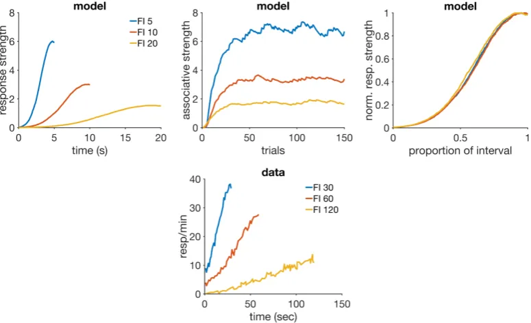
4.9 VI and FI . . . 91
Simulations . . . 92
Discussion . . . 92
4.10 Temporal Averaging . . . 94
Simulations . . . 94
Discussion . . . 96
4.11 Trace Conditioning . . . 97
Simulations . . . 98
Discussion . . . 100
5 Discussion 105
5.1 RWDDM Mechanisms . . . 105
5.2 Comparison with CSC-TD, MS-TD, LeT and MoT . . . 107
5.3 Limitations and Future Work . . . 108
5.4 RWDDM and Machine Learning . . . 111
6 Conclusion 115
List of Figures
2.1 Schematic representation of classical conditioning theories. When a CSi is present it activates its respective neuron-like unit Xi. Each CS unit is connected to the main response unitYby modifiable linksVi. The US unitz is also connected toY but by an unmodifiable linkλ. Adapted from Vogel, Castro and Saavedra,2004. . . 8 2.2 An idealized stimulus representation as it would be produced if a
physical stimulus with constant intensity was presented from 1 to 4 seconds. . . 8 2.3 Two theories of stimulus representation. Dashed lines are only active
when A and B are presented as a compound. Arrowheads represent excitatory connections whilst dotted ends are inhibitory. Note that the only structural difference between the two models is that in the replaced elements units Ab and Ba are also connected to the US. Ad-apted from Williams,2014. . . 15 2.4 TD learning model with a complete serial compound (CSC) stimulus
representation. In this representation both the onset and offset of the CS are instantiated by different xunits. The subscripts ijkrepresent the CS(i), the onset or offset (j) and the order of activation (k). Adap-ted from Vogel, Castro and Saavedra,2004. . . 18 2.5 The choices of stimulus representation in TD. Left panel: presence.
Middle panel: complete serial compound. Right panel: microstimuli. . 19 2.6 SOP model network. Arrows represent excitatory connections and
circles inhibitory. Adapted from Brandon, Vogel and Wagner (2002, p. 237). . . 20 2.7 The attention-modulated associative network. Arrows indicate
excit-atory connections and dots inhibitory. Adapted from Harris and Live-sey,2010. . . 24 2.8 The S-D model. Its network architecture includes a ‘hidden’ unit H.
This hidden unit is what allows the S-D model to explain negative patterning. . . 27 2.9 A three-node network used by the McLaren model. The nodes are
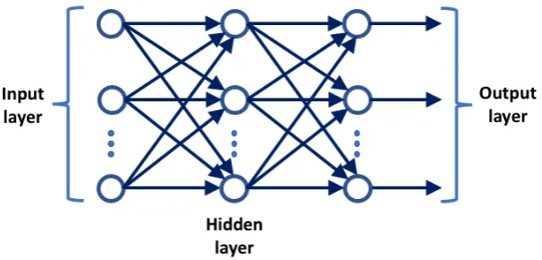
2.10 The perceptron. Each featurexiof the input is directly connected to a summing unit via modifiable linksVi. A bias unit of arbitrary value bwhich can be adjusted manually to improve the prediction is also connected to the summing unit. Note the similarity to the diagram of figure 2.1.. . . 31 2.11 A fully-connected hidden layer perceptron network. . . 33 2.12 LSTM. The memory block is the basic unit of processing in an LSTM.
Its inputs are the bias b, the CS and US values and the one time-step delayed output y. These are weighted and passed through a sigmoid function, before being multiplied by the output of the Input gate. The recurrent memory cell c1 adds this signal to the product of its own time delayed signal and the forget gate signal. Thec1output is passed through another sigmoid function and multiplied by the signal com-ing from the output gate, and the result is the memory block output y. The gates the same inputs as the memory block, and also the output ofc1which is delayed in the case of input and forget gates but not for the output gate. . . 38 2.13 An information processing flowchart of Scalar Expectancy Theory.
Counts from the pacemaker are accumulated in the working memory. A comparator compares the current count with a previously stored target count in reference memory. When the current count reaches the target count it triggers a response (‘yes’). Adapted from Allman et al.,
2014. . . 42 2.14 The basic structure of BeT and LeT. The presence of an external
stimu-lus initiates activity over a series of internal states (top). Each internal state is connected to a response unit (bottom) via modifiable associat-ive links. Adapted from Machado, Malheiro and Erlhagen,2009.. . . . 45 2.15 An example of the neural circuit in Spectral Timing Model. Each
separate CS activates a neuronal unitxi. Each of these units release neurotransmitteryi which will act on an intermediary neuronal layer. This intermediary layer is connected to the output node via modifi-able synapseszi. Adapted from Grossberg and Schmajuk,1989. . . 49 2.16 Flow diagram of Modular Theory. Reproduced from Guilhardi, Yi
and Church,2007. . . 52
3.2 RWDDM timer and CS representation during three 12-trial timing scenarios. Top two rows: timing a novel 6 second stimulus. Timer starts with a low baseline slope (A = 0.001) on trial 1 and gradu-ally adapts over training to reach approximately the required slope. Middle two rows: stimulus duration change from 6 to 3 seconds. Bot-tom two rows: stimulus duration change from 6 to 12 seconds. Para-meters:αt =0.215,θ =1,σ=0.25,m=0.15. . . 58
4.1 Acquisition and reacquisition. Top left: simulated associative strength Vin acquisition and extinction. Top middle: adaptation of RWDDM slope A. CR extinction began at trial 80 but has no effect on the RWDDM slope. Top right panel: simulatedV curves in acquisition and reac-quisition. Bottom left panel: response strength data from an exper-iment in acquisition and extinction, redrawn from figure 1 in Ricker and Bouton,1996. Bottom right panel: data from an experiment in ac-quisition and reacac-quisition, redrawn from the top panel of figure 3 in Ricker and Bouton,1996. Model parameters:m=0.15,θ =1,σ=0.3, αt =0.1,αV =0.1,H=4 in acquisition andH=0 in extinction. . . 69 4.2 Time change in extinction. Left column: simulated response strength
averaged over trials in extinction short-long (top) and long-short (bot-tom). Middle column: time estimate adaptation of the model during extinction short-long (top) and long-short (bottom). Right column: ex-perimental data from an experiment where the CS duration changed from 12-sec in acquisition to either 24-sec (top) or 6-sec (bottom) in ex-tinction. Data plots redrawn from figure 10 in Drew, Walsh and Bal-sam,2017. Model parameters: m = 0.25,θ = 1,σ = 0.35,αt = 0.08, αV =0.09,H=30. . . 72 4.3 Extinction curves. Left panel: modelVvalues for each CS duration in
4.4 Latent Inhibition. Top row: simulated associative strength in latent inhibition (left), simulated CR averaged over the first 30 trials of con-ditioning phase (middle), and simulated CR averaged over the last 30 trials of conditioning phase (right). Bottom row: acquisition curves from an actual experiment in latent inhibition (left), and response rate data during the CS (right). Data plots redrawn from figures 1 and 2 respectively in Bonardi, Brilot and Jennings, 2016. Model paramet-ers: αt = 0.1,αV = 0.08, µ = 1, σ = [0.6−0.35], m = 0.2, H = 4, αPH =0.4,γ=0.03.. . . 75 4.5 Experimental designs from two blocking experiments. CS X was blocked
(B) in rows 1 and 2, and not blocked (NB) in rows 3 and 4. Blue bar indicates US presence. . . 79 4.6 Blocking with different durations. Left column: simulation (top) with
a 15 sec blocking CS and 10 sec blocked CS, and animal data (bottom) from an experiment with the same design. Right column: simulation (top) with a 10 sec blocking CS and 15 sec blocked CS, and animal data (bottom) from an experiment with the same design. Data panels redrawn from the top right panel in figure 5 in Jennings and Kirk-patrick,2006. Model parameters: αt =0.2,αV =0.1,µ= 1,σ= 0.35, m=0.2,H=10. . . 80 4.7 Conditioned inhibition. Left column: simulation (top) and data
(bot-tom) from conditioned inhibition with a long inhibitor. Right column: simulation (top) and data (bottom) from conditioned inhibition with a short inhibitor. Data plots redrawn from figure 4 Williams, Johns and Brindas,2008. Model parameters: αt = 0.09,αV = 0.06,µ = 1, σ=0.35,m=0.16,H=30. . . 83 4.8 Disinhibition of delay and compound peak procedure. Top row:
sim-ulation (left) and data (right) of disinhibition of delay. Bottom row: simulation (left and middle) and data (right) of a compound peak pro-cedure. The middle panel is a normalized (proportion of maximum response strength) version of the left panel. Data plot redrawn from figure 13 in Meck and Church, 1984. Model parameters: m = 0.25,
θ =1,σ=0.18,αt=0.75,αV =0.1,H=5. . . 86 4.9 ISI effect. Top row: simulated average response rate during CSs (left),
4.10 Mixed FI. Left: simulated response strength during long trials. Right: response strength data from a mixed FI experiment, redrawn from figure 3 in Leak and Gibbon,1995. Model parameters: αt =0.2,αV = 0.1,µ=1,σ=0.425,m=0.2,H=30. . . 90 4.11 VI and FI. Top row: simulated average response strength during peak
trials (left), and the same data plotted after both axes are normal-ized (right). Bottom row: average response strength data from an experiment in VI and FI, redrawn from figure 1 in Matell, Kim and Hartshorne, 2014. Model parameters: αt = 0.1, αV = 0.1, µ = 1, σ=0.3,m=0.2,H=40.. . . 93 4.12 Temporal averaging. Top row: simulated response strength averaged
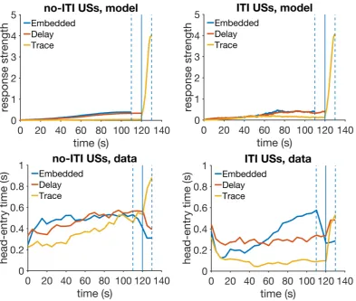
over peak trials in temporal averaging (left), and the same data nor-malized by maximum response strength and peak time (right). Bot-tom row: peak trial response strength data from an experiment in temporal averaging, redrawn from figure 1 in Swanton, Gooch and Matell,2009. Model parameters:αt = 0.2,αV =0.1,µ= 1,σ = 0.35, m=0.2,H=30. . . 95 4.13 Trace, embedded and delay conditioning. Top row: simulated
re-sponse strength averaged over 30 trials for the no-ITI USs (left) and the ITI USs groups. Bottom row: experimental data redrawn from fig-ure 2 in Williams et al.,2016. Model parameters: αt = 0.1,αV = 0.07, µ=1,σ=0.4,m=0.15,H =40. . . 99 4.14 Simulated associative strength in trace conditioning. The values for
List of Tables
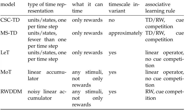
3.1 Summary of the main features of the models. . . 65
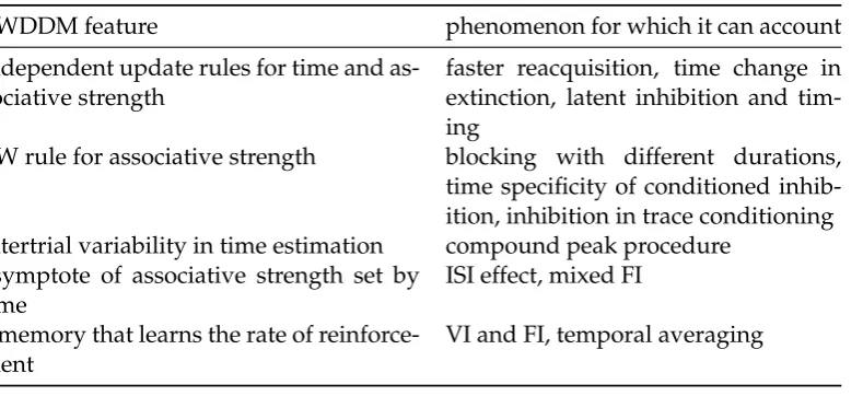
4.1 Model features and the experimental findings they can explain. . . 68 4.2 Simulation designs. . . 102 4.3 Summary of main simulation results and comparison with other
List of Abbreviations
BeT Behavioural Theory of Time CSC Complete Serial Compound CS Conditioned Stimulus CR Conditioned Response CV Coefficient of Variation E Excitatory
I Inhibitory
ISI Inter Stimulus Interval LeT Learning to Time LSM Least Means Squares
LSTM Long Short-Term Memory network MS-TD Microstimulus Temporal Difference MLP Multi-Layer Perceptron
MoT Modular Theory MTS Multiple Time Scales
O Organism
RW Rescorla-Wagner
RWDDM Rescorla-Wagner Drift-Diffusion Model S-D Schmajuk-DiCarlo Model
SET Scalar Expectancy Theory STM Spectral Timing Model
SOP Sometimes Opponent Processes or Standard Operating Procedures SSCC Simultaneous and Serial Configural-cue Compound
TD Temporal Difference
TDDM Timing Drift-Diffusion Model
TILT Timing from Inverse Laplace Transform US Unconditioned Stimulus
List of RWDDM Mathematical
Symbols
Ψ accumulator or timer
A accumulator rate
m accumulator noise factor θ accumulator threshold
t time
t∗ time of US occurrence
αt accumulator slope learning rate
x stimulus representation
σ standard deviation of the stimulus representation
V associative strength
H motivational parameter for the US αV associative strength learning rate
Chapter 1
Introduction
Classical conditioning theories aim to understand how associations between stimuli are learned. Ever since Pavlov,1927the process of association formation has been understood to depend crucially on the temporal relations between stimuli (Savast-ano and Miller,1998; Balsam, Fairhurst and Gallistel, 2006; Kirkpatrick,2013). Yet, classical conditioning theories have so far struggled to work when time is taken into account as an attribute of the stimulus representation. The study of time as a men-tal representation is the object of a separate area of study known as interval timing. Interval timing theories have produced a rich variety of time representations (Gib-bon, Church and Meck,1984; Killeen and Fetterman,1988; Machado,1997; Staddon and Higa,1999; Matell and Meck,2004), and therefore are a natural place to look for ways to integrate time into classical conditioning. In this thesis I first analyse previ-ous efforts in this direction before introducing a new hybrid classical conditioning and timing model.
Niv,2008; Niv,2009; Eshel,2016). However it is important to note that there is still no widely accepted complete neural mechanism for classical conditioning and that most theories stay at the computational level of explanation.
Stimulus representations are generally thought of as neural activation that is eli-cited by the stimulus, which may linger for a short time as a ‘trace’ after stimulus offset. Representations are commonly one of two types: molar or componential. Molar (or elemental) trace theories treat the stimulus as a single conceptualized unit whose activity is usually assumed to peak quite early following stimulus onset, and then gradually decrease (Hull,1943; Wagner,1981; Sutton and Barto,1981; Schmajuk and Moore,1988; McLaren and Mackintosh,2000; Harris and Livesey,2010). In con-trast, componential trace theories break down the CS representation into smaller units, each capable of being associated with the US, with some units more active early during the CS and others late, but all leaving a trace after activation (Desmond and Moore,1988; Grossberg and Schmajuk,1989; Vogel, Brandon and Wagner,2003; Ludvig, Sutton and Kehoe,2008).
Learning rules may be classified according to different criteria. An important period in the recent history of the field gave rise to one of these criteria. Prior to 1970’s conditioning used to be rooted in the stimulus-response tradition, which at-tributed crucial importance to the temporal pairing, or contiguity, of stimuli for the development of associations. The linear operator learning rule (Hull,1943) is one of the products of that period. In the late 1960’s and early 1970’s important experi-mental discoveries using compound stimuli, that is, a stimulus formed by combining other individual stimuli, showed the contiguity view to be incomplete (Kamin,1968; Rescorla,1988; Gallistel and Gibbon,2001). These compound experiments indicated that the formation of associations also depended on the reinforcement history of the individual elements forming the compound stimulus. This led to the development of new learning rules (Rescorla and Wagner,1972; Mackintosh, 1975a; Pearce and Hall,1980) capable of combining individual reinforcement histories in compounds, which the linear operator rule cannot. The first, and arguably still the most influen-tial, of these learning rules is the Rescorla-Wagner (RW, Rescorla and Wagner,1972). It has become famous for being the first model able to provide an account for the blocking effect (Kamin,1968), where a novel CS does not become associated with the US if it is reinforced only in compound with a previously conditioned CS.
forth explanations for timescale invariance and other timing properties (how time is encoded, how it is stored in memory and how it gets translated into behaviour) by recourse to an internal pacemaker. The most influential pacemaker-based timing theory to date is Scalar Expectancy Theory (SET, Gibbon, Church and Meck, 1984; Gibbon and Church,1984). The pacemaker is supposed to mark the passage of time by emitting pulses. These pulses can be gated to an accumulator via a switch which closes at the start of a relevant interval and opens when the interval is finished. The accumulator count is kept in working memory. At the end of the interval the current count is transferred to a long-term reference memory. Behaviour is guided by the action of a comparator which actively compares the count in working memory to the one retrieved from reference memory.
In spite of the considerable overlap, interval timing and classical conditioning are not easily integrated. Most conditioning theories are trial-based, that is they con-sider the trial as the unit of time. A trial is generally taken to be the state where a CS is present (or CSs in compound) and which may or may not contain a US (or USs). The most influential model in this category is the Rescorla-Wagner (RW, Rescorla and Wagner,1972). In order to account for different stimulus durations, trial-based theories like RW must resort to some sort of time discretization, usually by sub-dividing the trial into ‘mini-trials’. Each mini-trial is treated as a trial in its own right, which are then used to update associative links. This gives rise to the problem of deciding on a particular discretization. Also, given that humans experience time passing as a continuous flow, it is unlikely that animals discretize their conditioning experience in such a way. A more realistic approach to timing is taken by real-time theories. These theories attempt to formalize the concept of a continuous flow of time.
The Temporal Difference model (TD, Sutton and Barto,1990; Sutton and Barto,
brain may be employing a large number of neurons to represent it, but to dedicate so many resources only for timing might not be the most energy-efficient strategy. Also, TD and its stimulus representations do not usually account for a change in timing that is not tied to reinforcement. Animals time the occurrence of different events, such as onset and offset of stimuli (see for example Meck and Church,1984), but TD usually only allows for the timing of rewards.
On the other hand, timing models have made even fewer attempts at integrat-ing aspects of classical conditionintegrat-ing. A notable exception is the Learnintegrat-ing to Time (LeT, Machado,1997; Machado, Malheiro and Erlhagen,2009) model. It represents the passage of time by transitioning between internal states according to a stochastic pacemaker, an idea borrowed from an earlier timing model called the Behavioural Theory of Time (Killeen and Fetterman,1988). Learning takes place by associating reinforcement presentation with the current internal state according to the linear operator, a standard classical conditioning rule. LeT offers an account of the basic dynamics of association formation, but it cannot explain cue-competition phenom-ena like blocking. In a blocking procedure, a CS is first paired with a US until a CR is acquired. The same CS is then presented together with a novel CS and both are paired with the US for a few trials. If the novel CS is now presented alone it elicits little or no responding, and so it is said to be blocked by the first CS. LeT’s learning rule, the linear operator, has largely been supplanted by RW in classical condition-ing modellcondition-ing because it cannot explain cue-competition phenomena. Like TD, LeT also employs a representation that requires as many units as time-steps, making it a resource-intense model.
Modular Theory (MoT, Guilhardi, Yi and Church, 2007; Kirkpatrick,2002) is a timing model which because of its explicit goal of integrating timing and learning may be called a hybrid theory. MoT has introduced novelties that allow it to account for some aspects of the dynamics of classical conditioning that LeT cannot. Its archi-tecture is different than the connectionist one (states or units connected by modifi-able links) assumed by RW, TD and LeT. Instead, it uses a more cognitive architec-ture, with separate information processing stages that deal with perception, memory and decision. It postulates two separate memories: a pattern memory which stores CS durations, and a strength memory which stores the associative strength between each pattern memory and the US. This separation allows MoT to deal with more complex situations involving the dynamics of learning during acquisition and ex-tinction. However, MoT also relies on the linear operator to update its strength memory, which, like LeT, prevents it from accounting for cue-competition phenom-ena.
time in real-time. Like MoT and unlike LeT and TD, its time representation does not require an arbitrary large number of units or states. Similarly to TD but unlike LeT and MoT, it uses a learning rule that preserves the main features of RW which allow it to account for compound phenomena. It can time the onset and offset of all stim-uli, not only of rewards, and store a memory for each. It includes two update rules: one for timing that is updated by time-markers (such as stimulus onset/offset), and another for associations that is updated by the US. Hence, simple stimulus exposure causes the model to learn and store its duration. This capability is not present in models that depend only on an associative learning rule to also learn about time, such as TD and LeT.
This new model is essentially a way to connect one of the most influential clas-sical conditioning theories, the Rescorla-Wagner model (Rescorla and Wagner,1972), with a recently developed timing theory called Timing Drift-Diffusion Model (TDDM, Rivest and Bengio, 2011; Simen et al., 2011). The TDDM is based on the drift-diffusion model, widely used in decision making theory, and it provides an adaptive time representation that has commonalities with pacemaker-based models like SET and LeT (Simen et al.,2013). These models postulate the existence of a pacemaker that emits pulses at a regular rate, which are then counted to mark the passage of time. To preserve timescale invariance they either postulate a specific type of noise in the memory saved for intervals and a ratio-based decision process (SET) or adapt the rate of pulses (LeT). The TDDM takes the latter route but sets a fixed threshold on pulse counting. To emphasize the unification of these two theories I call our pro-posal the Rescorla-Wagner Drift-Diffusion Model (RWDDM).
1.1
Outputs
1.1.1 Conference Presentations
• Presentation at the XXVI (2014) International Congress of the Spanish Society
for Comparative Psychology (Braga, Portugal).
• Presentation at the XXVII (2015) International Congress of the Spanish Society
for Comparative Psychology (Seville, Spain).
• Presentation at the 2016 Associative Learning Symposium (Gregynog Hall,
Wales).
1.1.2 Publications
• Luzardo, A., Alonso, E., & Mondragón, E. (2017). A Rescorla-Wagner
Drift-Diffusion Model of Conditioning and Timing. PLOS Computational Biology, vol: 13 (11) pp: e1005796.
• Luzardo, A., Rivest, F., Alonso, E., & Ludvig, E. A. (2017). A drift–diffusion
model of interval timing in the peak procedure. Journal of Mathematical Psy-chology, 77, 111–123.
1.1.3 Code
Chapter 2
Literature Review
2.1
Learning Theories
The ability to learn relationships between different stimuli and events is an import-ant adaptive mechanism. In order to survive and reproduce an organism must be able to search for food and mates in an environment that is constantly changing al-beit with certain regularities. An organism that is able to learn from these regularities will maximise its chances of survival and reproduction.
Traditionally, two distinct types of associative learning have been recognized: classical (or Pavlovian) and operant (or instrumental) conditioning. In classical con-ditioning an association is believed to be formed between a stimulus (S) and a re-sponse (R), or between a stimulus and another stimulus. In operant conditioning an association is believed to be formed between R and an outcome (O). However the current tendency in the study of learning is to regard the associative structure underlying both S-R, S-S and R-O as fundamentally similar (Gallistel and Gibbon,
2000; Hall,2002). A strict distinction therefore will not be made between these two procedures here.
This section will review the main learning models, with a focus on their formal-isms. These are all connectionist models in the sense that they consist of nodes (or units) which represent the CS and US, and associative links (connections) between these nodes (see figure2.1 for a generic scheme). As Brandon, Vogel and Wagner,
2002remarked,
in such theories, the major theoretical options are centred around three questions. How shall the CSs and USs be represented? How shall the links between stimulus representations be construed to change during conditioning? How do the measures of conditioned responding depend on the current values of the stimulus representations and their associat-ive links? (p. 233)
FIGURE2.1: Schematic representation of classical conditioning theor-ies. When a CSi is present it activates its respective neuron-like unit
Xi. Each CS unit is connected to the main response unitYby
modifi-able linksVi. The US unitzis also connected toYbut by an
unmodi-fiable linkλ. Adapted from Vogel, Castro and Saavedra,2004.
2.1.1 Stimulus Representation
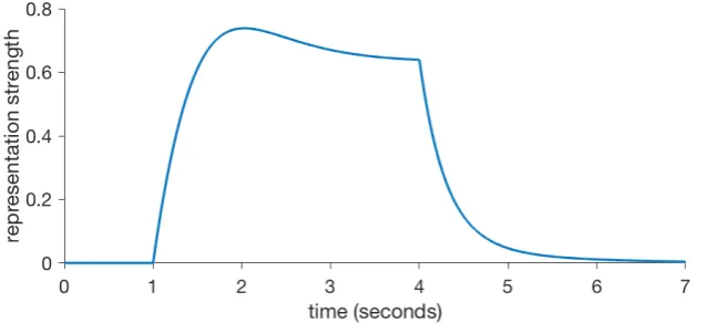
Stimulus representation is the problem of finding how the brain codes external phys-ical stimuli. This has a long history, going back to the beginning of experimental psy-chology with early behavioural theorists like Pavlov and Hull. Hull,1943adopted thestimulus-tracehypothesis of Pavlov, the idea that an external stimulus generates an internal representation that grows in strength at first, decays slowly until the physical stimulus is gone and then persists for a while as a rapidly decaying trace. Figure2.2shows a theoretical example. By and large, similar versions and variations of this simple concept have been adopted by every major learning theory to this day.
FIGURE2.2: An idealized stimulus representation as it would be pro-duced if a physical stimulus with constant intensity was presented
[image:33.595.146.465.536.682.2]A theoretical question arises: what is the fundamental unit of stimulus repres-entation? Is every CS and US to be independently represented or should they share common elements? Learning theories that take the first approach are known as ele-mentaland the latter asconfigural. Configural models are broader in scope than ele-mental ones, as they are able to handle stimulus generalisation and discrimination effects.
2.1.2 Learning Rules
How are the changes in learning actually instantiated? The vast majority of models are based on a theoretical construct calledassociative strengthrepresented by the letter
V. Vis conceptualized as a modifiable link between the CS and US representations (or, as in figure2.1, between the CS and an adaptive unit which is also connected to the US).
Historically, temporal contiguity was considered to be a necessary and sufficient cause of learning. It was thought thatV, to use modern terminology, increased only when CS and US occurred together. This view was shown to be too simplistic. Based on the work of Rescorla,1967, Balsam, Drew and Gallistel,2010and Balsam and Gal-listel,2009have argued that temporal contiguity is neither necessary nor sufficient and give two examples. Experiments with conditioned inhibition, where the US is presented only in the absence of the CS (see for example Rescorla,1969), can turn the CS into an inhibitor and hence demonstrate that temporal contiguity is not ne-cessary. Experiments with blocking (Kamin, 1968), where a CS fails to acquire a CR when it is paired both with a US and with another CS that has already been conditioned, shows that simple temporal contiguity is not sufficient. What these au-thors (Rescorla,1967; Balsam and Gallistel,2009; Balsam, Drew and Gallistel,2010; Gallistel, Craig and Shahan, 2014) argue is that contingency (correlation), and not contiguity, is the critical basis of learning. As it will be demonstrated later, one of the most successful learning rules, the Rescorla-Wagner rule, was devised as an attempt to capture contingency.
2.1.3 Response Rules
The ongoing difficulty and uncertainty in identifying neural substrates has meant that the most reliable way to assess learning continues to be through behaviour. However, this approach necessarily introduces confounds. Motivation or other factors can interfere with behaviour, thus distorting the expression of learning. Because of this theorists commonly make a distinction between learning and performance.
Learning models generally incorporate a rule that translates associative strength
V(a measure of learning) into responseY(a measure of performance). This rule may take the form of a simple multiplication, for example
whereXstands for the CS representation. Variations are of course possible such as the inclusion of a threshold on the value ofV below which learning is assumed to be too low to be translated into performance.
2.1.4 Trial-based Models
Trial-based learning models consider the trial as the fundamental unit of time. What constitutes a trial for these models will sometimes vary but it is usually defined as the period between CS onset and US onset.
One of the first, and still most influential, trial-based theories is the Rescorla-Wagner Model (RW, Rescorla and Rescorla-Wagner, 1972). It consists of an error-correction rule that adjusts the level of associative strengthVbetween the internal representa-tions of the CS and US:
∆Vi =αiβj zjλj−
∑
iXiVi
!
Xi. (2.2)
with
Xiorzj =
1 if CSior USj is present
0 if CSior USj is absent.
Constantsαi andβjare parameters related with the CSiand USjrespectively, which together determine the learning rate.
RW’s main achievement is in the assumption that all CSs currently present com-pete for a limited associative strength set by the US. This is what allows RW to ex-plain some cue-competition phenomena such as the blocking effect (Kamin,1968). In blocking, a CS1 is first conditioned alone and then it is presented in compound with a CS2. Despite receiving reinforcement during the compound phase, when the CS2is presented alone it does not elicit a response. RW can readily explain this with its competition for association assumption. V1, the associative strength of CS1, is at asymptotic level (V1 = 1) at the start of the compound phase, i.e. it has acquired all the available associative strength carried by the US, and henceV2does not change:
∆V2=α2β(1−X1V1−X2V2)
=α2β(1−1−0)
=0.
This competition mechanism also explains summation. Here two CSs are first paired separately with the same US until acquisition is complete (it is assumed that
2002, p. 207). Equation (2.2) predicts this will happen, since in the beginning of second phase:
∆V1 =∆V2=αβ(1−X1V1−X2V2),
=αβ(1−1−1),
=−αβ,
and hence bothV1 andV2 will decrease until they equal each 0.5, half of the US’s associative strength. Using a similar reasoning it is easy to see that RW also predicts superconditioning, an increased CR strength that occurs when a CS is paired with a US and another inhibitory CS (Williams and McDevitt,2002).
Another one of RW’s successes over its predecessors is that it can explain correla-tional experiments. Conditioning strength is positively correlated to the probability of the US in the presence of CS and negatively correlated to the probability of US in the absence of CS (Rescorla,1968). Here CS2stands for situational cues (the con-text) which is alone present during the intertrial interval and in compound with CS1 during the trial. The asymptotic associative strength of CS1, CS2and the compound CS1+2are (Rescorla and Wagner,1972):
V1 =V1+2−V2, (2.3)
V2 =
π2βp
π2βp−(1−π2)βa
, (2.4)
V1+2 =
π1+2βp
π1+2βp−(1−π1+2)βa, (2.5)
whereπ2andπ1+2 are the probabilities of reinforcement during CS2 and CS1+2 re-spectively, andβa andβp are the US parameters in the absence and presence of
re-inforcement respectively. If for exampleπ2= π1+2we haveV2 =V1+2(by (2.4) and (2.5)) and therefore by (2.3)
V1=0,
in other words, when the probability of US is the same both in the presence and absence of the CS, this CS does not acquire any associative strength, a prediction that is matched by experimental results (Rescorla,1968).
Conditioned inhibition is also readily explained. Here the US is only present in the absence of the CS, henceπ2 = 1 andπ1+2 = 0. By (2.4) and (2.5),V2 = 1 and
RW has some known limitations. Its main problem is with extinction of condi-tioned inhibitors. A prediction of the theory says that when an inhibitory CS is re-peatedly presented alone its associative strength should increase towards zero and hence lose its inhibitory characteristics. This is because an inhibitory CS has negat-iveV and so (0−V)will be positive, increasing V towards zero. This prediction however fails to hold experimentally (Zimmer-Hart and Rescorla, 1974). A com-mon solution is to consider conditioned excitation and inhibition as two distinct processes, each with their own associative strength: VE andVI. VE is updated only
when(zjλj−∑XiVi) > 0 andVI only when(zjλj−∑XiVi) > 0 (see for example
equation 11 in Brandon, Vogel and Wagner,2003). Finally, a single-unit RW model, as depicted in figure2.1, cannot explain negative patterning. In this conditioning phenomena, two different CSs signal reward but a compound formed by both of them does not. Animals learn to discriminate appropriately, but a single-unit RW fails to reproduce this behaviour. The answer is to add a second, hidden, unit whose outputs will serve as the input to an output unit (see figure2.8). I will have more to say about negative patterning and its importance to learning when I cover Artificial Neural Networks in section2.1.6.
Looking at the problem from a different angle, Mackintosh,1975aproposed an attention-based theory of learning. It is constructed from an established assumption in theories of selective attention, namely that an organism will pay more or less attention to a stimulus to the extent that this stimulus is a better or worse predictor of changes in reinforcement than the other stimuli available. Attention therefore is assumed here to be not just an intrinsic property of the CS but to also change with experience. This should be contrasted with the assumption in RW thatα, a learning rate that is related to the attentional properties of the CS, is constant. Mackintosh’s model operates by adjusting α so as to increase it when the CS becomes a better predictor of the US, and decrease otherwise. Formally,∆αi >0 if
|zλ−XiVi|<
zλ−
∑
XjVj(2.6)
and∆αi <0 if
|zλ−XiVi| ≥
zλ−
∑
XjVj(2.7)
where∑XjVjis the sum of associative strength of all CSs present in the trial except
CSi. The change inαis made proportional to the discrepancySbetween|zλ−XiVi|
and|zλ−∑XjVj|,
∆αi =S·αi. (2.8)
The change in associative strength is given by
It can be seen that Mackintosh’s model departs from RW in two ways: it turns an at-tention parameter from a constant into a variable, and it makes this parameter, and not RW’s CS competition for associative strength, capture CS contingency. Mack-intosh’s model provides an alternative explanation to blocking and overshadowing (where two equally salient CSs compete for associative strength). Whilst RW ex-plains these phenomena by invoking CS competition for a limited amount of associ-ative strength, Mackintosh’s theory uses a principle of learned irrelevance. In both cases, one of the CSs becomes a redundant signal of US, either because it doesn’t predict anything new (blocking) or because it is less salient and hence conditions more slowly (overshadowing).
Following Mackintosh, Pearce and Hall,1980proposed a model that is also based on the idea that experience can produce changes in CS effectiveness. They point out RW’s failure in explaining two variations in the classical blocking experiment. In the first, blocking was attenuated when in the compound phase the CSs were paired with a milder US than in the CS alone phase (Dickinson, Hall and Mackintosh,1976). In the second, blocking was not observed after only one trial was given with the com-pound (Mackintosh,1975b). These phenomena, the authors argue, support Mackin-tosh’s theory that learning involves a change in CS effectiveness. But as the authors also point out, Mackintosh’s model, like RW, does not effectively deal with latent inhibition, the retardation in learning that occurs when a CS is first presented alone before conditioning. The solution proposed by Pearce and Hall (PH) is to aban-don the idea that conditioning depends on CS competition for limited associative strength set by US (which can also be stated, as the authors do, as a change in US effectiveness) adopted by both RW and Mackintosh, and to rely solely on Mackin-tosh’s idea of changes in CS effectiveness. Unlike Mackintosh, which assumed that a CS is more effective if its a good predictor of its consequences, PH assumes the opposite: a CS is more effective to the extent that it is not an accurate predictor of its consequences. This is formalized as follows:
αni =
zλ
n−1−
∑
XiVin−1
, (2.10)
or in words, the CS associability parameter (or learning rate as in RW) in the present trialnis a consequence of how well the CS predicted reinforcement in the last trial
n−1. The authors acknowledge that such a one-trial change may be too fast and suggest that a moving average could be used instead, but the principle is the same. Change in associative strength is given by
∆Vi =Si·αi·λ (2.11)
whereSi is a constant that depends on CS salience. Consider as an example how
introduced it will therefore take longer for this CS to acquire associative strength than a CS that has not been pre-exposed. A few limitations have been identified since the model has first been proposed. Hall,2008notes that the results obtained in Mackintosh,1975bblocking experiment have not been replicated, and that more research showed some blocking does occur even in the very first trial. This lends support to RW’s interpretation.
The models described so far are called elemental, i.e. they treat each stimulus representation as an independent element. From this assumption it follows that if two CSs, say A and B, were conditioned separately (A+, B+ where ‘+’ means the US is present) and then presented together as the AB compound, their associative strengths should simply add up. This assumption was challenged by the negat-ive patterning experiment. In this preparation, the subject is asked to discriminate between conditions A+, B+ and a compound AB− where ‘−’ means the US is not present. Studies show that the subject is able to make such a discrimination, albeit not quickly, demonstrating that CSs interact in a more sophisticated fashion than the simple summation of RW.
An alternative way is to conceive of a compound as aconfiguration. Pearce,1987
developed a theory where configuration and generalization play a central role. In this theory A, B, and AB are all taken as configurations, each represented by a distinct neuron-like unit, with AB sharing half of its elements with each A and B. Pearce’s theory makes a further assumption, that the salience of all configurations is equal. This model solves negative patterning because AB is now an independent unit which enters into association with the US.
Wagner and Brandon,2001have proposed an equivalent componential version of Pearce, 1987 model and called it inhibited elements. They have also advanced their own componential stimulus representation called replaced elements (Brandon, Vogel and Wagner,2000). See figure2.3 for diagrams of these two stimulus repres-entation theories. These theories will not be evaluated further here since they do not add much to the question of time in learning central to this thesis, except to say that they propose to address issues that the simple adding of stimulus in RW does not contemplate.
(A) Inhibited elements
(B) Replaced elements
FIGURE2.3: Two theories of stimulus representation. Dashed lines are only active when A and B are presented as a compound. Arrow-heads represent excitatory connections whilst dotted ends are inhibit-ory. Note that the only structural difference between the two models is that in the replaced elements units Ab and Ba are also connected to
2.1.5 Real-time Models
Because trial-based models compress the whole duration of a trial to one single time point they cannot account for real-time changes in behaviour, the core of many tim-ing phenomena.
Real-time models attempt to describe behaviour as it unfolds. They will be de-scribed here either in differential or difference equations.
TD
Arguably, the most influential real-time learning model to date is the Temporal Dif-ference (TD; Sutton and Barto,1990; Sutton and Barto,1998). TD builds on the idea of expectation of US as a time derivative computation, first introduced by the same authors in an earlier model known as S-B (Sutton and Barto,1981). S-B will be dis-cussed first as it provides an introduction to TD.
Sutton and Barto, 1981 made an attempt to update adaptive neural networks with the principles discovered in animal learning theory. These two areas had been developing in parallel and with little contact. Sutton and Barto theorized that some internal processing analogous to cellular activity inside a neuron must take place in-side an adaptive unit (Yin figure2.1). This activity is described as a trace generated by the weighted average ¯Yof ongoing activityY,
¯
Y(t+1) =βY¯(t) + (1−β)Y(t). (2.12) If a US is presentY(t) =1+∑iXiVi, if US is absentY(t) =∑iXiVi. CSi is
represen-ted by another trace, called eligibility trace:
¯
Xi(t+1) =αX¯i(t) +Xi(t), (2.13)
whereαis a trace decay constant. It is assumed thatXi =1 when CSiis present and
0 otherwise. Change in associative strength is computed by
∆Vi(t+1) =c[Y(t)−Y¯(t)]X¯i(t), (2.14)
wherecis a learning rate.
conditioning, where a CS1 previously conditioned with a US can make a CS2 also acquire some associative strength when it is paired with CS1. Barto and Sutton,1982 demonstrated that S-B can produce conditioned inhibition.
Sutton and Barto, 1990identified problems with S-B’s account of the ISI effect and proposed a solution. Under more realistic simulations S-B predicted that a CS would become strongly inhibitory if simultaneously presented with US (ISI=0). This contradicts the data which shows that in this condition the CS actually becomes excitatory. Another problem was that S-B predicted equal conditioning strength for almost all ISIs in delay conditioning, whilst the ISI effect predicts a decay in strength with ISI. The solution they proposed was the Temporal Difference (TD) model.
TD introduces the idea of discounted future rewards into the time derivative S-B model. TD assumes that future rewardsλ are less valuable and so should be discounted in proportion to their distance from the present moment. It then creates a prediction ¯Vof the sum of these discounted rewards,
¯
V(t) =λ(t+1) +γλ(t+2) +γ2λ(t+3) +... (2.15) whereγis a discount factor. The authors then derive a replacement for S-B’s rein-forcement term[Y(t)−Y¯(t)]as follows. First they note that:
¯
V(t) =λ(t+1) +γλ(t+2) +γ2λ(t+3) +...
=λ(t+1) +γ(λ(t+2) +γ2λ(t+3) +...)
=λ(t+1) +γV¯(t+1). The time derivative of prediction therefore is
λ(t+1) +γV¯(t+1)−V¯(t). (2.16) Substituting this for[Y(t)−Y¯(t)]into (2.14) yields the TD learning rule:
∆Vi(t+1) =c[λ(t+1) +γV¯(t+1)−V¯(t)]X¯i(t). (2.17)
Figure2.4shows a diagram of TD.
Sutton and Barto,1990showed that TD can fix the problems in S-B and provide a better account of ISI effect in both delay and trace conditioning. They also demon-strate how it can exhibit blocking and second-order conditioning. It can also repro-duce the resistance to extinction of a conditioned inhibitor if the following condition is made:
¯
V=
∑iXiVi if ∑iXiVi >0
0 otherwise.
FIGURE 2.4: TD learning model with a complete serial compound (CSC) stimulus representation. In this representation both the onset and offset of the CS are instantiated by different x units. The sub-scriptsijkrepresent the CS(i), the onset or offset (j) and the order of
activation (k). Adapted from Vogel, Castro and Saavedra,2004.
TD has found many applications in the field of artificial intelligence and adapt-ive control (Sutton and Barto,1998) and constitutes the basis of modern deep learn-ing algorithms (Mnih et al.,2015). It has received a particular boost in popularity in the field of neuroscience. Schultz, Dayan and Montague,1997have shown that dopaminergic neurons fire in anticipation of a reward in a manner resembling TD predictions.
Ludvig, Sutton and Kehoe,2008proposed a stimulus representation to be used with TD with the aim of refining its timing predictions. Even though CSC-TD could explain some timing phenomena, it was not able to explain timescale invariance. This timing phenomena refers to the finding that the timing of the CR tends to scale with stimulus duration. Microstimuli (MS), as the representation is called, formal-ises the CS as a series of Gaussians
f(y,µ,σ) =√1 2π
exp
−(y−µ)2
2σ2
, (2.19)
whereyis an exponentially decaying trace set at 1 at CS onset. The ith microstimulus is given by:
Xi(t) = f(y(t),i/m,σ)y(t), (2.20) wheremis the total number of microstimuli. The right panel in figure2.5shows the structure of microstimuli.
FIGURE2.5: The choices of stimulus representation in TD. Left panel: presence. Middle panel: complete serial compound. Right panel:
microstimuli.
2.5). It is arguably the most basic representation but it is able to explain the ISI effect on conditioning (Sutton and Barto,1990). But since it represents absolute temporal generalization, it cannot account for the intertrial temporal dynamics. The other TD stimulus representation is theComplete Serial Compound(CSC) first proposed by Moore, Choi and Brunzell,1998. In CSC the CS is composed of a series of neuron-like units, one for each time-step (see middle panel in figure2.5). Such a representation is not very realistic in terms of neurophysiology as it postulates the existence of an arbitrarily large number of neuron-like units, but it is a clear improvement on the presence representation as shown by Sutton and Barto, 1990. Ludvig, Sutton and Kehoe,2012demonstrated that microstimuli fared the same or better than the other representations on the ISI effect, CR timing, CR scalar invariance, blocking, block-ing with a change in ISI and overshadowblock-ing. The authors point out that TD with MS cannot account for certain phenomena such as discrimination, preexposure and recovery.
SOPs
if the CS is still present. The change in the proportion of elements in states A1, A2 and I are given by:
∆pA1= p1(pI)−pd1(pA1) (2.21) ∆pA2= pd1(pA1)−pd2(pA2) (2.22) ∆pI = pd2(pA2) (2.23)
wherepA1,pA2andpIare the proportion of elements in states A1, A2 and I
respect-ively. These equations produce a stimulus representation for A1 activation similar to the one in figure2.2.
FIGURE2.6: SOP model network. Arrows represent excitatory con-nections and circles inhibitory. Adapted from Brandon, Vogel and
Wagner (2002, p. 237).
The stimulus representation in SOP allows the model to reproduce habituation effects. Brandon, Vogel and Wagner,2003simulated repeated presentations of the US, demonstrating that the model produces weaker URs with massed US training, an effect well-known empirically.
SOP’s learning rules are:
∆Vi+= L+
∑
i
pA1,CSi×pA1,USj for excitatory learning, (2.24)
∆Vi−= L−
∑
i
pA1,CSi×pA2,USj for inhibitory learning, (2.25)
∆Vi =∆Vi+−∆Vi−, (2.26)
whereL+,L− are constants. The modifiable associative strengthV is the net result of inhibitoryV−and excitatoryV+strengths.
given by
p2US/∑CS = i
∑
VCSiUS(r1pA1CSi+r2pA2CSi)wherer1,r2are constants andp2 is restricted to the interval (0,1). ResponsesRin the model are generated by:
R= f(w1pA1,US+w2pA2,US), (2.27)
wherew1,w2are constants. The precise function f is left to be defined by data fits. Brandon, Vogel and Wagner,2003showed that SOP can produce changes in as-sociative strength compatible with acquisition, extinction and cue competition, in a similar manner as Rescorla-Wagner. They also argue SOP is the only model to predict inhibition with backwards conditioning.
In its original formulation SOP does not adequately predict timing phenomena. Brandon, Vogel and Wagner,2003attributes this failure to SOP’s unitary stimulus representation. Their simulations showed that SOP predicts optimal conditioning with simultaneous CS and US presentation, whilst the data show a minimum ISI is required for optimal conditioning. It does not predict the correct CR timing; its associative strength peaks too early into the trial at the end of training.
Two other variations of SOP have been proposed. The first, called AESOP for affective extension of SOP (Brandon, Vogel and Wagner,2003), postulates two sep-arate units for the US representation, one emotive and the other sensory-perceptual. The emotive unit gives rise to a conditioned emotive response (CER), a diffuse re-sponse that is believed to regulate the CR. The sensory-perceptual unit supports the CR. Apart from this novel US representation, AESOP maintains the assumptions of SOP.
The main advantage of AESOP over SOP is in dealing with CERs. Indeed, the motivation behind its development was to explain the phenomenon called ‘diver-gence of response measures’. It refers to the observation that different measures of conditioned response may yield contrary, or uncorrelated, results. For example, backward eyelid conditioning produces inhibitory learning when eyeblinks are the measure of conditioning but produces excitatory learning when suppresion of drink-ing is measured. Such phenomena can be accounted by the two distinct US nodes in AESOP. By using different decay constants for these units, AESOP can also correctly account for the ability of CERs to develop at longer ISIs than CRs.
reinforced when presented alone) the procedure is called a feature positive discrim-ination. Conversely, if the target CS is not reinforced when preceded by the feature CS the procedure is called a feature negative discrimination. If feature and target do not overlap, i.e. are presented serially, then the feature CS is said to act as an ‘occa-sion setter’ for the target CS. The occa‘occa-sion setter is seen as conveying information about the impending target. Of particular interest here is temporal information. A feature CS may indicate that the target CS will come after a certain time interval, what is called a feature-target interval (FTI).
Holland, 1998 performed a series of experiments with FTIs ranging from 5 to 50 seconds. Their results were in line with data obtained in the peak procedure (a common experiment in the timing literature) in that the response curves obtained with different FTIs superimposed when appropriately scaled. Of particular interest are compound features experiments. In a particularly interesting mix of cue com-petition and timing, Holland,1998presented a 10/30 second feature compound and then either the 10 or 30 target CS. The response curves looked very similar to each other (Figure 2 in Holland,1998), with two apparent peaks, the first higher than the second and both shifted to the right of the target intervals. This points to a kind of time subtraction in the compound feature cue. One way to interpret this result is that the internal clock was slowed down by the compound cue.
As mentioned above, C-SOP is an attempt at providing an explanation for the type of timing phenomena seen in occasion setting and CR timing. SOP represented the CS as a set of elements that can be in one of three states, and its learning rules (equations (2.24) and (2.25))are applied to the whole sets. C-SOP applies these rules directly to the elements. These are assumed to have value 1 when active and 0 when inactive. C-SOP also introduces the assumption that some elements are temporally correlated, showing consistency from trial to trial. Hence, in C-SOP the CS elements belong to one of two classes, one temporally correlated and another randomly dis-tributed.
Brandon, Vogel and Wagner, 2003argue that C-SOP treats the question of CR timing as one analogous to an AX+, BX−discrimination. Elements that are active during US presentation become excitatory, the ones active only in the absence of the US become inhibitory and the ones active at both times become moderately excit-atory. The CS trace is built by adding them at each time step. It is also assumed that each element can carry a limited amount of inhibitory or excitatory associative strength, so thatl− ≤ vi ≤ l+. Finally, a constrained version of the RW learning
rules is used:
∆Vi =
αβ+(λ−∑vi)(l+−vi) if(λ−∑vi)>0,
αβ−(λ−∑vi)(vi−l−) if(λ−∑vi)<0,
(2.28)
where|l|<λ.
and Wagner, 2003 showed that the model can reproduce the ISI effect, CR timing and timescale invariance of CR timing.
Harris
Harris and Livesey, 2010 presented a model that relies heavily on a neural com-putation known as divisive normalization. This is accomplished by dividing the responses of an individual neuron by the summed activity of a pool of neurons. Normalization is considered an ubiquitous neural computation that may underlie the modulatory effects of visual attention, the encoding of value and the integration of multisensory information (Carandini and Heeger,2012).
Because the normalization equation is so central to the model, it will be useful to explain it in detail first. The basic idea is that the normalized response of a neuron
Rjis given by (Carandini and Heeger,2012):
Rj =
Dnj
σn+∑kDnk (2.29)
whereDjis the neuron’s input,σa constant andDkthe input from the normalization pool which is considered not normalized. Informally, this equation means that in a background of strong activation it will take a stronger input to reach the same normalized response that a weaker input would produce in a background of weak activity.
Figure2.7shows a diagram of the model. A CS is thought to activate elements
E. Each element is sparsely connected to other elements (Harris and Livesey, 2010, made eachEconnected with half of the rest of elements in the network). EachE ac-tivates one inhibitory unitIand weakly activates another nearbyIunit. Unit Ithen normalizesEactivity (via inhibition) according to the backgroundEactivity. The CS also activates an attention networkAwhich inhibit unitsI. A second normalization occurs betweenA units via their own inhibitory connections. Associative strength
Vis carried by the connections betweenEunits.
Formally, the model describes the changes in activity strength of units E, I and
A. A distinction is made between two types of unit responses: a potential response
Rpotand an actual responseR. Their relationship is described by:
dR
dt =σ(Rpot−R), (2.30)
withσa constant. Accordingly, activation of unitEis given by:
dEx
FIGURE2.7: The attention-modulated associative network. Arrows indicate excitatory connections and dots inhibitory. Adapted from
Harris and Livesey,2010.
where
Epot=
Input(Ex)p
Input(Ex)p+Ixp+D
, (2.32)
Input(Ex) =
Sx+∑ni=1ViEi if(Sx+∑ni=1ViEi)>0
0 otherwise
(2.33)
wherep,Dare constants andSxexternal input (CS).
Activation of unitI is given by
dIx
dt =δ(Ipot−Ix), (2.34)
where
Ipot=
Input(Ix)p
Input(Ix)p+ (kaAx)p+D
, (2.35)
Input(Ix) = n
∑
i=1
zi,xEi. (2.36)
Herezi,xis the weight betweenEiandIx. This is taken to reflect the degree of
simil-arity between the receptive fields ofEi andEx. zx,xis set to 1, whilst every otherzi,x
is less than 1.
Activation of unitAis given by
dAx
where
Apot= S
p x
Spx+A
0p
x +D
, (2.38)
A0x=w "
n
∑
i=1
Ai
!
−Ax
#
, (2.39)
withwa constant.
Finally, associative strength is calculated in a manner that resembles S-B model, but the authors make one modification. Their rule intends to formalize the idea that associative change of the recipient element is proportional to the difference between the change in excitation and the change in inhibition. It also incorporates the idea of a change in salience or associabilityαcommon to the trial-based attention models. First, a function that determines the co-activation of elementsExandEyis calculated
by:
∆x,y =αx
βE
dEy
dt −βI dIy
dt
, (2.40)
where
βE =
0.02 if dEdty >0,
0 otherwise, (2.41)
βI =
0.1 if dIdty >0,
0 otherwise. (2.42)
Then to make the change in associative strength a gradual process the authors use a rule that changes the acceleration ofV:
d2Vx,y
dt2 = kν
∆x,y−
dVx,y
dt
, (2.43)
withkνa constant. Also, the change in associability is given by:
dαx
dt = kα(Ex−αx), (2.44)
wherekαis a constant.
so the model can cope well with non-linear cue competition phenomena. The au-thors also demonstrate that the model can produce latent inhibition because of its attentional network and its rule for associability modification. Crucially, the latent inhibition produced by the model is not due to US absence, as models like Mackin-tosh,1975awould require, but simply because of a decrement in CS processing, in a manner similar to the model by McLaren and Mackintosh,2000.
It is worth noting at this point that this model’s formalism has more biological realism than it is usually seen in learning models. Its timing properties, however, remain untested.
Schmajuk
Schmajuk and colleagues have proposed several connectionist models, one of which (Buhusi and Schmajuk,1999) is of particular interest here due to its timing features. It is a blend of two previous models: the Schmajuk-DiCarlo (S-D, Schmajuk and DiCarlo,1992) and the Spectral Timing (STM, Grossberg and Schmajuk,1989) mod-els. STM is primarily a timing model and will be covered in more detail in the next chapter. It suffices to state here that its main timing engine is a cascade of traces set off by the CS, each trace with its own timing characteristics. S-D is a classical conditioning connectionist model, with a hidden-unit layer that allows it to account for certain stimulus configuration phenomena such as negative patterning that two-layer networks cannot explain.
The model builds on the idea that CSs compete not only for associative strength, the assumption behind Rescorla-Wagner, but also for US timing. Figure2.8shows the main components of the model. Each CSi sets offktracesτik, including the
con-text CX. These traces are formed by activitiesxikandyikgiven by1: ∆xik = k1
k (1−xik)(CS(i) +k2f1(i))−k3xik, (2.45)
∆yik =k4(1−yik)−k5f2(xik)yik, (2.46)
whereCS(i)is 0 or 1 depending on CS absence or presence respectively,kiare
con-stants controlling decay or growth, andfiare sigmoid functions. These two activities
are combined by the following rule:
τik =yikf2(xik). (2.47)
Equation (2.47) produces gaussian-looking traces, with higher peaks and smaller widths near CS onset. These traces are very similar in shape to the ones postulated by the Microstimuli model (see right panel in figure2.5).
1The following is an abridged description where some of the equations that do not form the core of
FIGURE2.8: The S-D model. Its network architecture includes a ‘hid-den’ unit H. This hidden unit is what allows the S-D model to explain
negative patterning.
These traces are fed into the second network layer seen in figure2.8, which in turn is connected to the hidden-unitHjand directly to the output layer by modifiable
linksV Hikj andVik respectively (except context CX which is only connected to the
hidden unit). The learning rule forVikis
∆Vik =k11τik(US−BUS)(1− |Vik|) (2.48)
whereBUSis the aggregate US prediction produced by the second and hidden layers
BUS=
∑
i∑
kτikVik+
∑
j
τjV Nj. (2.49)
Note the term(1− |Vik|)in equation (2.48). This term preventsVik, the direct
associ-ative link between CS and output layer, from changing whenVik =±1. It also
mod-ulates the learning rate so as to make it faster whenVikis further from its asymptotic
value. The learning rule for the hidden-unit linkV Hikjis
∆V Hikj =k13τikτj(US−BUS)V Nj. (2.50)
The output of the hidden unit is the traceτjcomputed as follows:
τj =k8f4
∑
i
∑
kτikV Hikj
!
. (2.51)
Finally, the hidden-unit linkV Njwith the output unit is updated by
∆V Nj =k12τj(US−BUS)(1− |V Nj|), (2.52)
As mentioned earlier, this model assumes competition between tracesτfor the timing of US. Traces that peak closer in time to reinforcement receive more strength and come to dictate response topography. It is this feature that allows the model to reproduce the basic ISI effect. Another important feature is the two independent CS connections, one directly to the US representation and another indirectly via the hidden unit. According to Buhusi and Schmajuk,1999this independence allows the CS to act both as a simple CS (via direct link) and as an occasion setter (via hidden unit). It is this last property that allows the model to explain stimulus configuration phenomena.
Adding to the list of successful conditioning paradigms simulated in Schmajuk and DiCarlo,1992with its successor S-D model, which include acquisition of delay and trace conditioning, extinction, blocking, overshadowing, generalisation, and negative and positive patterning, Buhusi and Schmajuk,1999showed that this model can reproduce temporal and associative properties of blocking and serial feature positive discrimination.
McLaren
McLaren and Mackintosh,2000and McLaren and Mackintosh,2002set out to show that an elemental model is also capable of explaining generalization and discrim-ination, a class of phenomena frequently thought to require a configural stimulus representation. The inclusion of a weight decay in its associative links allows the model to also explain some timing properties.
Their starting point is a distributed network model of information processing and memory (McClelland and Rumelhart, 1985). This type of model consists of highly interconnected units, activated both by external stimuli or internal stimuli originating from other units. A CS is therefore here represented as a pattern of ac-tivation distributed over the network. As with other connectionist models, learning occurs through a change in connection weights. This change is guided by the delta rule:
∆i =ei−ii,
whereeandiare external and internal activations respectively. Learning therefore is interpreted here as the network trying to match (or equalize) external activity with internal activity. When these are equal, learning is complete.
McLaren and Mackintosh, 2000 make two main modifications on McClelland and Rumelhart,1985. First, they include a positive feedback mechanism in the delta rule, which has a modulatory effect on the salience of external stimuli. Second, they introduce the idea of weight decay; weights change with experience but also decay with time. This modification allows the model to reproduce ITI effects.
external. The sum of internal inputs arriving at unit i from unit j is given by:
ii =
∑
wjiΩj. (2.53)Activation in node i is symbolized byΩjand changes according to:
dΩi
dt =
E(ei+ii)(1−Ωi)−DΩi forΩ≥0
E(ei+ii)(1+Ωi)−DΩi otherwise
(2.54)
where D and E are decay and excitation constants respectively. The delta rule is modified to include the modulation termr∆,ra constant, as follows:
∆i = (ei+r∆i)−ii. (2.55)
The modulation constantr is taken to be 0 when ∆i ≤ 0. Finally, the weights are
adapted according to the following system:
dwij
dt =S∆iΩj−Kmij, (2.56) dmij
dt =S∆iΩj−Lmij, (2.57)
with constantsL>K. Equation (2.57) is a negative feedback that implements weight decay.
FIGURE2.9: A three-node network used by the McLaren model. The nodes are fully interconnected by the linkswi,j, and also receive
ex-ternal inputsei.