Enforcing Eigenvector Smoothness for a Compact
DFT-based Polynomial Eigenvalue Decomposition
Fraser K. Coutts
∗, Keith Thompson
∗, Jennifer Pestana
†, Ian K. Proudler
∗, Stephan Weiss
∗∗ Department of Electronic & Electrical Engineering, University of Strathclyde, Glasgow, Scotland † Department of Mathematics & Statistics, University of Strathclyde, Glasgow, Scotland
{fraser.coutts,stephan.weiss}@strath.ac.uk
Abstract—A variety of algorithms have been developed to compute an approximate polynomial matrix eigenvalue decom-position (PEVD). As an extension of the ordinary EVD to poly-nomial matrices, the PEVD will generate paraunitary matrices that diagonalise a parahermitian matrix. While iterative PEVD algorithms that compute a decomposition in the time domain have received a great deal of focus and algorithmic improvements in recent years, there has been less research in the field of frequency-based PEVD algorithms. Such algorithms have shown promise for the decomposition of problems of finite order, but the state-of-the-art requires a priori knowledge of the length of the polynomial matrices required in the decomposition. This paper presents a novel frequency-based PEVD algorithm which can compute an accurate decomposition without requiring this information. Also presented is a new metric for measuring a function’s smoothness on the unit circle, which is utilised within the algorithm to maximise eigenvector smoothness for a compact decomposition, such that the polynomial eigenvectors have low order. We demonstrate through the use of simulations that the algorithm can achieve superior levels of decomposition accuracy to a state-of-the-art frequency-based method.
I. INTRODUCTION
The expression of broadband multichannel problems via polynomial matrix representations [1] has been identified as a viable approach for broadband beamforming [2], [3], broad-band angle of arrival estimation [4]–[6], and polyphase anal-ysis and synthesis matrices for filter banks [7]. Parahermitian polynomial matrices, which are identical to their parahermitian conjugate, i.e., R(z) = R˜(z) = RH(1/z∗) [7], are often central to these applications, and can arise as the z-transform of a space-time covariance matrix: R(z) =P
τR[τ]z−τ. A polynomial matrix eigenvalue decomposition (PEVD), which is defined in [8] as an extension of the eigenvalue decomposition to parahermitian matrices, uses finite impulse response (FIR) paraunitary matrices [9] to approximately di-agonalise a space-time covariance matrix. Given an input para-hermitian matrixR(z)∈CM×M, and its associated coefficient matrix R[τ], PEVD algorithms generate an output diagonal matrixD(z)containing eigenvalues, and a paraunitary matrix Q(z)containing eigenvectors, such that
D(z)≈Q˜(z)R(z)Q(z). (1) Equation (1) has only approximate equality, as the PEVD of a finite order polynomial matrix is generally not of finite order. Note that the decomposition in (1) is unique up to permuta-tions and arbitrary allpass filters applied to the eigenvectors, provided thatQ(z)andD(z)are selected analytic [10].
Existing PEVD algorithms include second-order sequential best rotation (SBR2) [8], sequential matrix diagonalisation (SMD) [11], and various evolutions of the algorithm fami-lies [12]–[14]. These algorithms employ iterative time domain schemes to approximately diagonalise a parahermitian matrix,
and typically encourage spectral majorisation [15] such that the resulting eigenvalues are ordered.
A DFT-based PEVD formulation, which transforms the problem into a pointwise-in-frequency standard matrix decom-position, is provided in [16]. The method can either return a spectrally majorised decomposition, or attempt to approximate maximally smooth eigenvalues. This algorithm has been shown to perform well for finite order problems [17], but requires an a priori guess of the length of the paraunitary matrix Q(z)in the decomposition.
Here, we present a novel frequency-based PEVD algorithm which can compute an accurate PEVD without requiring an es-timate of the paraunitary filter length. It has been demonstrated in [10] that the lowest order approximation to (1) is possible if we attempt to approximate analytic eigenvectors which — on the unit circle — are characterised by being infinitely differentiable. We utilise a cost function that measures the power in derivatives based on the Fourier coefficients of their discrete samples on the unit circle. This permits us to maximise eigenvector smoothness for a low order decomposition.
Below, Sec. II and Sec. III will introduce the smoothness metric and the proposed algorithm, respectively. A comparison of the algorithm’s performance relative to the method in [16] is presented in Sec. IV, with conclusions drawn in Sec. V.
II. SMOOTHNESSMETRIC
A PEVD produces eigenvaluesλm(ejΩ) and eigenvectors qm(ejΩ), where λm(ejΩ) is the mth diagonal element of D(z)|z=ejΩ andqm(ejΩ)is the mth column of Q(z)|z=ejΩ.
For the eigenvectors qm(ejΩ) to be compact in the time domain, they must be maximally smooth on the unit circle [10]. In this section, we propose a novel metric to measure the smoothness of eigenvectors.
If K is sufficiently large and odd, the samples Fk = F(ejΩk),Ω
k= 2Kπk,k= 0. . .(K−1), of a function F(ejΩ) permit its reconstruction via the Dirichlet kernel P(ejΩ):
F(ejΩ) =XK−1
k=0 FkP(e
j(Ω−Ωk)), (2)
where
P(ejΩ) = 1
K ·
sin(K2Ω) sin(12Ω) =
1
K
XK−1
ℓ=0 e
−jΩ(ℓ−K−1 2 ). (3)
Thus,
F(ejΩ) = 1
K
XK−1
k=0 Fk
XK−1
ℓ=0 e
−j(Ω−Ωk)(ℓ−K2−1). (4)
For thepth derivative ofF(ejΩ), we have
dp
dΩpF(e
jΩ) = 1
K K−1
X
k=0
Fk
(K−1)/2
X
ℓ=−(K−1)/2
(−jℓ)pe−j(Ω−Ωk)ℓ.
We are interested in the power contained within the pth derivative of F(ejΩ),
χp=
1 2π Z π −π dp
dΩpF(e jΩ)
2
dΩ, (6)
which provides some measure of the smoothness ofF(ejΩ).
Note that due to orthogonality of the complex exponential terms and integration over an integer number of fundamental periods, for a Fourier series with arbitrary coefficientsaℓ,
1 2π Rπ −π P
ℓaℓejΩℓ
2
dΩ =P
ℓ21π
Rπ
−π
aℓejΩℓ
2
dΩ =P
ℓ|aℓ|2.
(7) Therefore, we can write
χp= 1 K2
X(K−1)/2
ℓ=−(K−1)/2
(−jℓ)
pXK−1
k=0 Fke
jΩkℓ
2 (8) = 1 K2
X(K−1)/2
ℓ=−(K−1)/2ℓ 2pfHC
ℓf =fHC(p)f , (9)
where f = [F0, F1,· · · , FK−1]T contains K frequency
sam-ples Fk =F(ejΩk),k= 0. . .(K−1),
Cℓ=
1 ej2π
Kℓ · · · ej 2π K(K−1)ℓ
e−j2π
Kℓ 1 ...
..
. . .. ...
e−j2π
K(K−1)ℓ · · · 1
, (10) and
C(p)= 1
K2
X(K−1)/2
ℓ=−(K−1)/2ℓ 2pC
ℓ. (11)
If we want to consider smoothness up to thePth derivative, we can form the metric
χ(P)=XP
p=1χp=f H
XP
p=1C (p)
f
=fH
1
K2
(K−1)/2
X
ℓ=−(K−1)/2
Cℓ P
X
p=1
ℓ2p
f =fHC(P)f ,
(12) which calculates the sum of all powers of derivatives off up to and including thePth derivative. For evenK, the derivation is similar to above and produces
χ(P)=fH
1
K2
K 2−1
X
ℓ=−K 2
Cℓ P
X
p=1
ℓ2p
f =fHC(P)f . (13)
III. PROPOSEDALGORITHM A. Overview
The PEVD approach presented here uses a frequency-based scheme to obtain a solution to (1). In the discrete frequency domain, this equation has the form
R[k] =Q[k]D[k]QH[k], k= 0,1, . . . , K−1, (14) whereQ[k]contains eigenvectors,D[k]contains eigenvalues, andR[k]is obtained from the K-point DFT ofR[τ], R[k] =R(z)|z=wk
K =
P
τR[τ]wkτK , k= 0,1, . . . , K−1, where wK = e−j2π/K. An approximate PEVD is therefore obtained via K independent EVDs.
Noting that the decompositions in (1) and (14) are only unique up to permutations and phase shifts [10], an advantage of the frequency-based approach proposed here is the option to rearrange the eigenvalues and eigenvectors at each frequency
bin if desired. If the eigenvalues in D[k] are arranged in de-scending order, approximate spectral majorisation of the result-ing polynomial eigenvalues occurs. A smooth decomposition, whereby both eigenvalues and eigenvectors are continuous in frequency, typically produces a more compact decomposition, but requires aditional effort. Sec. III-B discusses the method used to form a smooth decomposition.
Each eigenvector at each frequency bin can be influenced by an arbitrary scalar phase angle and still be valid. Discon-tinuities in phase between adjacent frequency bins can arise due to this ambiguity in eigenvector phase. When assessed via the metric of Sec. II, eigenvectors containing such phase discontinuities are not smooth and return high values ofχ(P). For a short paraunitary matrixQ(z), these discontinuities must be smoothed [10] andχ(P)decreased. This is achieved through
the use of a phase alignment function, described in Sec. III-C, which uses Powell’s ‘dogleg’ algorithm [18], [19] to maximise eigenvector smoothness.
Following the reordering (if desired) and phase alignment ofQ[k],Q[τ]is computed via the inverse DFT as
Q[τ] =PK−1
k=0 Q[k]w
−kτ
K , τ = 0,1, . . . , K−1, (15)
andD[τ]is found in a similar fashion.
B. Smooth Decomposition
In a smooth decomposition, the eigenvalues — and their eigenvectors — are arranged such that discontinuities between adjacent frequency bins are minimised. Such discontinuities can occur when the eigenvalues intersect at some frequencies. A relatively low complexity method for reordering the eigen-values and eigenvectors from [16] is used in this algorithm, and is described below.
For a smooth decomposition, the eigenvectors in adjacent frequency bins are rearranged using the inner product
cij[k] =qHi[k−1]qj[k], (16) where, qi[k]is the ith column ofQ[k]. For each eigenvector qi[k−1],i= 0. . . M−1, a subsequent eigenvectorqi′[k] is
chosen from an initial set S={0. . . M−1}of the columns ofQ[k]such that
i′= arg max
j∈S{|cij[k]|}, (17) Once i′ is identified, it is removed from the set: S = S − {i′}, and the next eigenvector is chosen. The selected eigenvectors are combined in a rearranged matrix Q′[k] = [q0′[k]. . .q(M−1)′[k]], and Q[k] is set equal to Q′[k]. The
eigenvaluesD[k]are rearranged according to the reordering of the eigenvectors. This process is completed fork= 1. . . K−1.
C. Phase Alignment
1) Overview: Phase alignment of eigenvectors in adjacent
frequency bins is vital for a compact-order decomposition. Phase alignment can be achieved by finding the phase changes required for each eigenvectorqm[k] ∀m, k to be maximally smooth according to metric χ(P). The phase of the mth
eigenvector at frequency bin k can be adjusted by an angle θk according toˆqm[k] =ejθkqm[k]. Below, we define an ob-jective function which, when minimised via an unconstrained non-linear optimisation algorithm, can be used to determine the optimalθk ∀kto maximise themth eigenvector’s smoothness.
2) Objective Function Formulation: The smoothness
to measure the smoothness of a single function. We wish to compute a vector of phases θ= [θ0, θ1,· · · , θK−1]T ∈RK×1
such that all elements of the mth eigenvectorqm[k]∀ k are maximally smooth. Our objective function therefore measures the smoothness of all elements of qm[k]and takes the form
f(θ) =R{XM−1 n=0 f
H
nC(P)fn} (18) where we choosefnH=vndiag{[ejθ0,· · ·, ejθK−1]}andv
n=
[qm,n[0],· · · ,qm,n[K−1]], where qm,n[k] denotes the nth element (row) of eigenvector qm[k] at frequency bink. Only the real component of the sum in the above equation is taken, as the imaginary component should be zero.
The above equation can be rearranged to form
f(θ) =R{uH M−1
X
n=0
diag{vn}C(P)diag{vHn}
!
u}, (19)
whereuH= [ejθ0,· · · , ejθK−1].
Setting Γ = PM−1
n=0 diag{vn}C(P)diag{vHn} ∈ CK×K allows for the following compact representation:
f(θ) =R{uHΓu}. (20) We therefore wish to obtainθ by solving
θ= arg minf(θ). (21)
3) Minimising the Objective Function: Given its simplicity
and relatively low cost [19], we employ Powell’s iterative ‘dogleg’ trust region strategy [18] for the unconstrained min-imisation of (20). In iterationi, a trust region strategy uses the gradient vector g and approximate Hessian matrix Hˆ of the objective function to construct a second-order Taylor model:
mi(ϕ(i)) =f(θ(i)) +ϕ(i)Tg+ϕ(i)THϕˆ (i). (22) This model approximatesf(θ(i)+ϕ(i))within a trusted region of radiusR(i)around the current pointθ(i)for some stepϕ(i), which is identified according to
ϕ(i)= arg min
ϕ(i)
mi(ϕ(i)) kϕ(i)k< R(i). (23)
The selected method first finds the minimiser of (22) along the steepest descent direction:
ϕ(ci)=− gTg
gTHgˆ g. (24)
If this point lies outside of the trusted region, the intersection of the line from the origin toϕ(ci)with the trust region boundary is used for ϕ(i). Otherwise, the quasi-Newton point is found: ϕ(qni)=−Hˆ−1g. (25)
If this point lies within the trust region,ϕ(i)=ϕ(i)
qn, and the method moves to the next iteration. Otherwise, a solution is found at the intersection of the trust region boundary with the line fromϕ(ci) toϕ(qni).
A parameter ρ, which compares the predicted reduction in the objective function with the actual reduction, is used to measure the strength of the approximation given by (22):
ρ=f(θ (i)
)−f(θ(i)+ϕ(i))
mk(0)−mk(ϕ(i))
. (26)
In practice, if ρ > 0.75, the approximation is good and the trust region is expanded. If ρ < 0.25, the approximation is poor and the trust region is decreased in size. Furthermore, if ρ >0,θ(i+1)=θ(i)+ϕ(i); otherwise,θ(i+1)=θ(i).
4) Gradient Vector and Hessian Matrix Formulation: The
objective function in (20) can also be written as
f(θ) =
K−1
X
i=0
K−1
X
k=0
u∗
iγikuk= K−1
X
i=0
K−1
X
k=0
γikej(θi−θk). (27)
Taking the derivative with respect toθℓ:
∂f ∂θℓ
=−j K−1
X
i=0,i6=ℓ
γiℓej(θi−θℓ)+j K−1
X
k=0,k6=ℓ
γℓkej(θℓ−θk)
=−j K−1
X
i=0
γiℓej(θi−θℓ)+j K−1
X
k=0
γ∗
kℓe−j(θk−θℓ). (28)
Note: γℓk = γkℓ∗ as Γ is Hermitian. Converting to matrix notation, the gradient vector is
g=∂f
∂θ =−jdiag{u}Γ
Tu∗+jdiag{uH}ΓHu
= 2R{jdiag{uH}ΓHu}=−2I{diag{uH}Γu}. (29) Taking the derivative of (28) with respect to θp, with θℓ now fixed, we get the equation for the off-diagonal elements of the Hessian matrix:
∂f ∂θℓ∂θp
=−j2γpℓej(θp−θℓ)−j2γpℓ∗e−j(θp−θℓ)
=γpℓej(θp−θℓ)+γpℓ∗e−j(θp−θℓ). (30) So the off-diagonal (OD) terms of the Hessian matrix are:
HOD= diag{u}ΓTdiag{u∗}+ diag{uH}ΓHdiag{u} = 2R{diag{uH}Γdiag{u}}. (31) Taking the derivative of (28) with respect to θℓ, we get the equation for the diagonal elements of the Hessian matrix:
∂2f
∂θ2
ℓ
=−
K−1
X
i=0,i6=ℓ
γiℓej(θi−θℓ)− K−1
X
k=0,k6=ℓ
γℓkej(θℓ−θk). (32)
In matrix form, this equates to
HD= diag{−diag{u}ˆΓTu∗−diag{uH}ΓˆHu} =−2R{diag{diag{u}ΓˆTu∗}}, (33) whereΓ = Γˆ −diag{diag{Γ}}contains zeroes on its diagonal. The Hessian matrix is then given by
H=HOD−diag{diag{HOD}}+HD = 2R{diag{uH}Γdiag{u}}
−diag
diag
2R{diag{uH}Γdiag{u}}
−2R{diag{diag{u}ΓˆTu∗}}
= 2R{diag{uH}Γdiag{u}}
−2R{diag{diag{Γ}+ diag{u}ΓˆTu∗}}
= 2R{diag{uH}Γdiag{u}} −2R{diag{diag{u}ΓTu∗}}, (34) since diagdiaguH Γdiag{u} =diag{Γ}.
The second part of (34) is typically less significant when compared to the first part; i.e.,
k2R{diag{diag{u}ΓTu∗}}kF
k2R{diag{uH}Γdiag{u}}kF ≈10
−3,
(35)
2R{diag{uH}Γdiag{u}} is positive semi-definite, as C(P) and Γ are positive semi-definite. We propose the following approximation to the Hessian matrix, which is guaranteed to be positive definite and eliminates unnecessary computation:
ˆ
H= 2R{diag{uH}Γdiag{u}}+αIK , (36) whereαis very small andIK is aK×K identity matrix.
D. Algorithm Complexity
The complexity of the phase alignment step for a single eigenvector is O(K3) due to matrix inversion [16]; thus,
the total complexity of the phase alignment step for M eigenvectors is of order O(M K3). The computation of the
frequency domain representation ofR[τ]∀τ, the execution of K EVDs, and the formulation of a smooth decomposition are of lower complexity than this step; thus, the total complexity of the proposed algorithm is approximately O(M K3).
IV. ALGORITHMPERFORMANCE
To benchmark the proposed approach against the existing method in [16], this section first defines performance metrics for evaluating the performance of PEVD algorithms before setting out two simulation scenarios, over which an ensemble of simulations will be performed.
A. Performance Metrics
Denote the mean-squared reconstruction error for an ap-proximate PEVD as
MSE = M12L′
P
τkER[τ]k2F, (37) where ER[τ] = Rˆ[τ]−R[τ] ∀ τ, Rˆ(z) = Q(z)D(z)Q˜(z), and L′ is the length of E
R(z). Furthermore, define the paraunitarity error as
η= 1
M P
τkEQ[τ]−IM[τ]k2F, (38)
where EQ(z) = Q(z)Q˜(z), IM[0] is an M ×M identity
matrix, and IM[τ] for τ 6= 0 is an M × M matrix of
zeroes. The output paraunitary matrix Q(z) can be used in signal processing applications; a useful metric for gauging the implementation cost of this matrix is its length,LQ.
B. Simulation Scenarios
The simulations below have been performed over an en-semble of103instantiations ofR(z)∈CM×M,M = 5, based on the randomised source model in [11]. In this source model, which generates ground truth D(z) and Q(z), the order of D(z)is 18 and the order of Q(z) is 10, such that the total order ofR(z)is 38. The dynamic range of the eigenvalues is constrained to ensure that the average is around50 dB.
The proposed algorithm considers smoothness up to the third derivative; i.e., we use the metric χ(3). A maximum of
50 minimisation steps according to Sec. III-C3 are allowed, and a parameter of α= 10−14is used.
1) Scenario 1: The method in [16], henceforth referred to
[image:4.612.321.569.64.179.2]as the ‘existing’ algorithm, requires knowledge of LQ prior to execution, and typically chooses a number of frequency bins Ke= 2LQ+L−2, where L is the length of the input matrix R(z). Our method, referred to as ‘proposed’, does not require an input value of LQ, but instead outputs Q(z) with length equal to the number of frequency bins Kp used in the decomposition. Note: outer lags of Q[τ] may contain negligible energy and can be trimmed using a thresholdµin a process detailed in [8]. The first scenario provides the existing
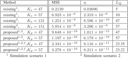
TABLE I. AVERAGEMSE,η,AND A POSTERIORILQCOMPARISON.
Method MSE η LQ
existing1
, Ke= 47 0.2139 0.03696 5
existing1
, Ke= 57 6.923×10⁻⁶ 2.319×10⁻⁶ 10
existing2
, Ke= 131 1.251×10⁻⁹ 8.596×10⁻¹⁰ 47
existing2
, Ke= 151 5.854×10⁻⁹ 3.296×10⁻⁹ 57
proposed1,2
, Kp= 47 9.648×10⁻¹⁸ 1.011×10⁻¹⁵ 47
proposed1,2
, Kp= 57 1.197×10⁻²² 6.179×10⁻¹⁹ 57
proposed1,2,‡,K
p= 47 2.341×10⁻¹⁰ 8.116×10⁻¹¹ 23.35
proposed1,2,‡,K
p= 57 3.278×10⁻¹⁰ 8.211×10⁻¹¹ 23.22
1
Simulation scenario 1 2
Simulation scenario 2 ‡Q[τ]truncated using thresholdµ= 10−10and scheme from [8]
method with values of LQ ∈ {5, 10}, and uses the same generated values ofKe=Kp∈ {47, 57}for both algorithms. Note that each algorithm is instructed to produce a smooth decomposition.
2) Scenario 2: To test the case where both algorithms
produceQ(z)of the same length, the second scenario provides the proposed method with values of Kp ∈ {47, 57}, and provides the existing method with LQ = Kp such that Ke∈ {131, 151}.
C. Results
The ensemble-averaged mean squared reconstruction error, η, and LQ were calculated for both algorithms for both simulation scenarios, and can be seen in Tab. I. The table demonstrates that the proposed approach is able to provide extremely low decomposition MSE and paraunitarity error. Furthermore, the existing method is not capable of achieving such performance even when using significantly more fre-quency bins and generating paraunitary filters of the same length. The algorithmic complexity of both algorithms is approximately O(M K3) [16], [17]; thus the choice of DFT
length K is extremely significant. Also shown is the impact of truncation on performance: if paraunitary filter length is of critical importance, then MSE and η can be sacrificed to generate shorter filters. Typically, increasing K is shown to improve MSE and η at the expense of higherLQ.
V. CONCLUSION
In this paper, we have introduced a novel frequency-based algorithm capable of computing a compact PEVD. This algo-rithm makes use of a newly developed metric for measuring the smoothness of a function on the unit circle. By minimising this metric for the eigenvectors produced by the algorithm, we have successfully modified the phase responses of the eigenvectors and enforced their compactness in the time domain.
Simulation results have demonstrated that the proposed al-gorithm offers superior performance to an existing frequency-based PEVD algorithm, with the advantage of not requiring a priori information regarding the paraunitary filter length.
When designing PEVD implementations for real applica-tions, the algorithm described in this paper could be extremely useful, provided that K is not prohibitively large.
ACKNOWLEDGEMENTS
Fraser Coutts is the recipient of a Caledonian Scholarship; we would like to thank the Carnegie Trust for their support.
REFERENCES
[1] I. Gohberg, P. Lancaster, and L. Rodman. Matrix Polynomials. Aca-demic Press, New York, 1982.
[2] S. Weiss, S. Bendoukha, A. Alzin, F. K. Coutts, I. K. Proudler, and J. Chambers. MVDR broadband beamforming using polynomial matrix techniques. InEUSIPCO, pp. 839–843, Nice, France, Sep. 2015. [3] A. Alzin, F. K. Coutts, J. Corr, S. Weiss, I. K. Proudler, and J. A.
Chambers. Adaptive broadband beamforming with arbitrary array geometry. InIET/EURASIP ISP, London, UK, Dec. 2015.
[4] M. Alrmah, S. Weiss, and S. Lambotharan. An extension of the music algorithm to broadband scenarios using polynomial eigenvalue decom-position. In19th European Signal Processing Conference, pp. 629–633, Barcelona, Spain, Aug. 2011.
[5] S. Weiss, M. Alrmah, S. Lambotharan, J. McWhirter, and M. Kaveh. Broadband angle of arrival estimation methods in a polynomial matrix decomposition framework. InIEEE 5th Int. Workshop Comp. Advances in Multi-Sensor Adaptive Proc., St. Martin, pp. 109–112, Dec. 2013. [6] F. K. Coutts, K. Thompson, S. Weiss, and I. K. Proudler. Impact of
Fast-Converging PEVD Algorithms on Broadband AoA Estimation. In
SSPD, London, UK, Dec. 2017.
[7] P. P. Vaidyanathan. Multirate Systems and Filter Banks. Prentice Hall, Englewood Cliffs, 1993.
[8] J. G. McWhirter, P. D. Baxter, T. Cooper, S. Redif, and J. Foster. An EVD Algorithm for Para-Hermitian Polynomial Matrices. IEEE TSP, 55(5):2158–2169, May 2007.
[9] S. Icart, P. Comon. Some properties of Laurent polynomial matrices. InIMA Int. Conf. Math. Signal Proc., Birmingham, UK, Dec. 2012. [10] S. Weiss, J. Pestana, and I. K. Proudler. On the Existence and
Uniqueness of the Eigenvalue Decomposition of a Parahermitian Matrix.
IEEE TSP, accepted for publication, 2018.
[11] S. Redif, S. Weiss, and J. McWhirter. Sequential matrix diagonalization algorithms for polynomial EVD of parahermitian matrices. IEEE TSP, 63(1):81–89, Jan. 2015.
[12] J. Corr, K. Thompson, S. Weiss, J. McWhirter, S. Redif, and I. K. Proudler. Multiple shift maximum element sequential matrix diagonalisation for parahermitian matrices. In IEEE Workshop on Statistical Signal Processing, pp. 312–315, Gold Coast, Australia, June 2014.
[13] F. K. Coutts, J. Corr, K. Thompson, I. K. Proudler, and S. Weiss. Divide-and-Conquer Sequential Matrix Diagonalisation for Parahermitian Ma-trices. InSSPD, London, UK, Dec. 2017.
[14] F. K. Coutts, K. Thompson, I. K. Proudler, and S. Weiss. Restricted Update Sequential Matrix Diagonalisation for Parahermitian Matrices. InIEEE CAMSAP, Curacao, Dec. 2017.
[15] P. Vaidyanathan. Theory of optimal orthonormal subband coders.IEEE TSP, 46(6):1528–1543, June 1998.
[16] M. Tohidian, H. Amindavar, and A. M. Reza. A DFT-based approximate eigenvalue and singular value decomposition of polynomial matrices.
EURASIP J. Adv. Signal Process., 2013:93, December 2013. [17] F. K. Coutts, K. Thompson, I. K. Proudler, and S. Weiss. A Comparison
of Iterative and DFT-Based Polynomial Matrix Eigenvalue Decomposi-tions. InIEEE CAMSAP, Curacao, Dec. 2017.
[18] M. J. D. Powell. A new algorithm for unconstrained optimization.
Nonlinear programming, pp. 31–65, 1970.