Copula selection models for non-Gaussian responses that are missing not at random

City, University of London Institutional Repository

Citation

: Gomes, M., Radice, R., Camarena Brenes, J. and Marra, G. (2019). Copula

This is the accepted version of the paper.

This version of the publication may differ from the final published

version.

Permanent repository link:

Link to published version

: http://dx.doi.org/10.1002/sim.7988

Copyright and reuse:

City Research Online aims to make research

outputs of City, University of London available to a wider audience.

Copyright and Moral Rights remain with the author(s) and/or copyright

holders. URLs from City Research Online may be freely distributed and

linked to.

Copula selection models for non-Gaussian responses

that are missing not at random

Manuel Gomes

Rosalba Radice

Jose Camarena Brenes

Giampiero Marra

Abstract

Missing not at random (MNAR) data poses key challenges for statistical inference

be-cause the model of interest is typically not identifiable without imposing further (e.g.,

dis-tributional) assumptions. Sample selection models have been routinely used for handling

MNAR by jointly modelling the outcome and selection variables assuming that these

fol-low a bivariate normal distribution. Recent studies have advocated parametric selection model

approaches, for example estimated by multiple imputation and maximum likelihood, that are

more robust to departures from the normality assumption. However, the proposed methods

have been mostly restricted to a specific joint distribution (e.g., bivariatet-distribution). This

paper discusses a flexible copula-based selection approach (which accommodates a wide range

of non-Gaussian outcome distributions and offers great flexibility in the choice of functional

form specifications for both the outcome and selection equations) and proposes a flexible

im-putation procedure that generates plausible imputed values from the copula selection model. A

simulation study characterises the relative performance of the copula model compared with the

most commonly used selection models for estimating average treatment effects with MNAR

data. We illustrate the methods in the REFLUX study, which evaluates the causal effect of

laparoscopic surgery compared to usual medical management on long-term quality of life in

patients with reflux disease. We provide software code for implementing the proposed copula

framework using theRpackageGJRM.

Key Words: copula, joint model, missing not at random, multiple imputation, non-Gaussian

outcome, selection model, simultaneous equation model.

1

Introduction

Missing data remains a major concern in clinical and epidemiological studies. In many settings,

the chances of observing the data tend to be associated with the (underlying) unobserved values of

the outcome of interest. For example, health-related quality of life outcomes are increasingly used

for assessing the benefits of health care interventions (NICE, 2013). However, these outcomes

are typically self-reported and a key concern is that the chances of completing the quality of life

questionnaire are likely to be related to patient’s true health status (after adjusting for the observed

data) (Mason et al., 2017). In such cases, the data is said to be missing not at random (MNAR),

and non-response must be modelled together with the substantive model for the observed data.

Selection models have been commonly used to handle MNAR data in clinical and

epidemio-logical research (e.g., Sales et al., 2004; Del Bianco & Borgoni, 2006; Alva et al., 2014), by jointly

modelling the outcome and missingness models typically assuming bivariate normality. Heckman

(1974) was one of the first to propose such model (Heckman selection model) using a

simultane-ous equation approach, where the error terms were assumed to follow a bivariate Gaussian. At

that time, to circumvent some of the difficulties associated with direct likelihood maximisation,

Heckman proposed a 2-stage least-squares estimation procedure (Heckman, 1979). This involved

combining a probit model for the probability of observing the outcome (1st stage) with a linear

regression model for the outcome (2nd stage), which was a function of the estimates obtained in

the 1st stage. Although this approach is somehow robust to deviations from normality (method of

moments estimator), it relies crucially on the availability of exclusion restrictions, i.e. variables

that predict missingness but are unrelated to the outcome of interest (Puhani, 2000).

An alternative approach to estimating selection models is the single-step full-information

max-imum likelihood (FIML) which jointly estimates the outcome and missing data equations. For

example, Diggle and Kenward (1994) combined a marginal model for the outcome with a logistic

outcome. The study used the Nelder-Mead optimisation algorithm, although in practice such

se-lection models may be more flexibly estimated by MCMC techniques in a Bayesian framework

(Daniels & Hogan, 2008). Alternatively, selection models can also be implemented with

multi-ple imputation (MI) (Galimard et al., 2016). Essentially, MI imputes a set of plausible values for

each missing observation, which are drawn from the posterior distribution of the missing values

conditional on the observed data. To handle MNAR, the imputed values can be obtained using a

selection model, such as the Heckman model, to recognise that the missing data may be related

to unobserved values. A recent study suggested that the FIML and MI approaches based on the

Heckman model are sensitive to departures from the assumption of Gaussian outcomes (Gomes

et al., 2017).

Recent studies have considered various generalisations to address possible deviations from

normality. For example, the Heckman selection model has been extended to accommodate data

with heavier tails by considering a bivariate t-distribution (Marchenko & Genton, 2012; Ding,

2014; Ogundimu & Collins, 2017), whereas Zhelonkin et al. (2015) introduced a procedure for

robustifying the Heckman’s two-step estimator by using M-estimators of Mallows’ type for both

steps. However, most of these approaches are restricted to a specific joint distribution for the

selection and outcome processes, and the extension to non-Gaussian outcomes may not be easy.

Semi-parametric (e.g., Lee, 2008; Chib et al., 2009; Newey, 2009) and non-parametric (e.g., Das

et al., 2003; Chen & Zhou, 2010) selection models have been proposed, but these have not

perme-ated practice as their implementation may be challenging in the regression context (Pigini, 2015).

This paper addresses some of these concerns by discussing a copula-based selection framework

which accommodates a wide range of non-Gaussian distributions, not restricted to the exponential

family. The link function for the copula’s selection equation is allowed to be different from the

classic probit, and the parameters of the copula and marginal distributions can be made

depen-dent on several types of covariate effects (e.g., linear, non-linear, random and spatial effects). In

principle, the approach allows for any parametric continuous marginal outcome distribution and

link function for the selection equation, and several dependence structures between the margins

as implied by copulae. While the copula approach is fully parametric, it is computationally more

al-lows the researcher to assess the sensitivity of results to different modelling assumptions. This

article then introduces a flexible imputation procedure that generates plausible imputed values

from the copula selection model. The proposed methods can be easily implemented using the

gjrm() function in the R package GJRM (Marra & Radice, 2017b), and we provide software

code to encourage the uptake of the methods (see the Supplementary Material online).

The plan for the remainder of the paper is as follows. In Section 2, we describe our motivating

example. Section 3 describes the original Heckman selection model and Section 4 discusses the

copula selection model framework and the proposed imputation procedure. Section 5 presents the

design and results of a simulation study that evaluates the relative merits of the copula approach

compared to commonly used selection models across different MNAR settings. Section 6 reports

the results from applying the methods to our case-study, and Section 7 discusses the findings in

light of previous methodological studies and provides directions for further research.

2

Motivating example

Gastro-Oseophageal Reflux Disease (GORD) develops when reflux of the stomach acid cause

troublesome symptoms or complications which adversely affect patients’ well-being. About

20-30% of adult ’Western’ populations experience heartburn or reflux intermittently, and many of

these patients are often treated with Proton Pump Inhibitors (PPIs) to suppress acid reflux. While

PPIs are generally effective, there is the concern that long-term acid suppression with PPIs may

be associated with increased risk of chronic hypergastrinaemia and gastric cancer. An alternative

to long-term medication is to have laparoscopic surgery, which is a minimally invasive procedure

but carries some risk of side effects. Our motivating example, the REFLUX study, compares these

interventions for treating patients with GORD in the UK. The REFLUX study was a pragmatic

randomised controlled trial, which included two components: a randomised component in which

patients were randomised to surgery and medical management, and a non-randomised

compari-son (according to patient preferences) between a policy of offering early surgery and a policy of

continued medical management; full details can be found in Grant et al. (2013). Our study

policy makers. The non-randomised preference arms included 261 patients for surgery and 192

in medical management. Self-reported quality of life was measured at baseline, 3 months and

then annually up to 5 years, using the EQ5D3L (measure anchored on a scale that includes 0

-death, and 1 - perfect health) questionnaire (EuroQol, 1990). The primary outcome of interest was

quality-adjusted life-years (QALYs), an outcome that combines both quality of life and survival,

measured at 5 years.

A significant proportion of patients failed to complete the EQ-5D-3L questionnaires, resulting

in missing 5-year QALYs for 55% (106 out of 192) of patients in the medical management group

and 48% (125 out of 261) in the surgery group. Baseline covariate information was mostly

com-plete. A key concern in this study was that the relative effectiveness of laparoscopic surgery vs

medical management may be sensitive to alternative assumptions about the missing data. More

specifically, trial coordinators suspected that patients in worse health in the control group lost

in-terest in the study (because the intervention was not working for them), and hence were less likely

to return quality of life questionnaires or answer the phone.

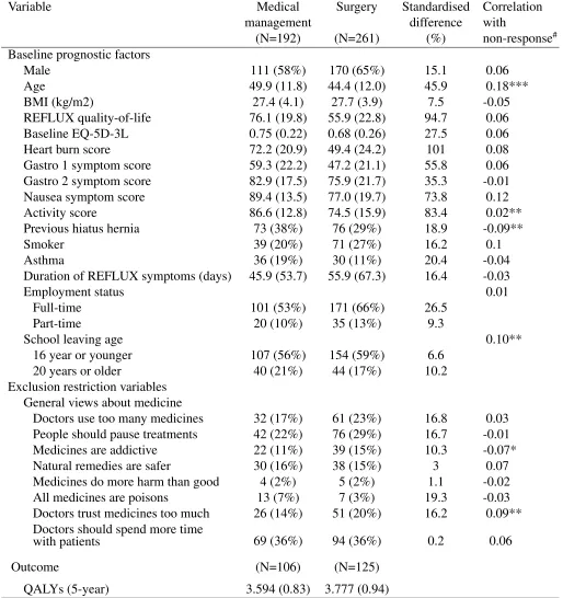
Table 1 provides a description of the main baseline covariates and their association with the

missing data indicator. This included key prognostic factors of the health outcome, which had large

imbalances between the intervention groups and were included in the substantive model, and a set

of variables that were predictive of missingness but anticipated to be conditionally independent

of the outcome, i.e. met the criteria for the ’exclusion restriction’. Missing data were strongly

associated with some key prognostic factors such as age and activity score, but weakly associated

with other the exclusion restrictions (views about medicine). This raises some pertinent questions

for the choice of selection model approach; for example, whether the relative merits of alternative

selection models differ according to the strength of association between the exclusion restriction

and non-response.

In addition, QALYs are typically left-skewed and often include negative values (reflecting

health states judged worse than death). This unusual distributional shape raises significant

chal-lenges to sample selection models, and existing approaches (which assume a bivariate normal

or t-distribution) are unlikely to be plausible in this context. Figure 1 suggests that a Gumbel

Table 1: Descriptive statistics of the baseline characteristics and their correlation with non-response, and the quality-adjusted life year (QALY) outcome.

Variable Medical Surgery Standardised Correlation

management difference with

(N=192) (N=261) (%) non-response# Baseline prognostic factors

Male 111 (58%) 170 (65%) 15.1 0.06

Age 49.9 (11.8) 44.4 (12.0) 45.9 0.18***

BMI (kg/m2) 27.4 (4.1) 27.7 (3.9) 7.5 -0.05

REFLUX quality-of-life 76.1 (19.8) 55.9 (22.8) 94.7 0.06 Baseline EQ-5D-3L 0.75 (0.22) 0.68 (0.26) 27.5 0.06 Heart burn score 72.2 (20.9) 49.4 (24.2) 101 0.08 Gastro 1 symptom score 59.3 (22.2) 47.2 (21.1) 55.8 0.06 Gastro 2 symptom score 82.9 (17.5) 75.9 (21.7) 35.3 -0.01 Nausea symptom score 89.4 (13.5) 77.0 (19.7) 73.8 0.12

Activity score 86.6 (12.8) 74.5 (15.9) 83.4 0.02**

Previous hiatus hernia 73 (38%) 76 (29%) 18.9 -0.09**

Smoker 39 (20%) 71 (27%) 16.2 0.1

Asthma 36 (19%) 30 (11%) 20.4 -0.04

Duration of REFLUX symptoms (days) 45.9 (53.7) 55.9 (67.3) 16.4 -0.03

Employment status 0.01

Full-time 101 (53%) 171 (66%) 26.5

Part-time 20 (10%) 35 (13%) 9.3

School leaving age 0.10**

16 year or younger 107 (56%) 154 (59%) 6.6

20 years or older 40 (21%) 44 (17%) 10.2

Exclusion restriction variables General views about medicine

Doctors use too many medicines 32 (17%) 61 (23%) 16.8 0.03 People should pause treatments 42 (22%) 76 (29%) 16.7 -0.01 Medicines are addictive 22 (11%) 39 (15%) 10.3 -0.07* Natural remedies are safer 30 (16%) 38 (15%) 3 0.07 Medicines do more harm than good 4 (2%) 5 (2%) 1.1 -0.02 All medicines are poisons 13 (7%) 7 (3%) 19.3 -0.03 Doctors trust medicines too much 26 (14%) 51 (20%) 16.2 0.09** Doctors should spend more time

with patients 69 (36%) 94 (36%) 0.2 0.06

Outcome (N=106) (N=125)

QALYs (5-year) 3.594 (0.83) 3.777 (0.94)

Notes: Continuous covariates (and outcome) reported as Mean (SD) and binary covariates as N (%). Belief variables are di-chotomised: 1 if patient agrees or strongly agrees with the statement, 0 otherwise.

#_{Pearson correlation coefficient between each variable and the binary missing data indicator. Statistical significance is based}

Histogram and Density of Response

Quality-adjusted life years (QALYs)

Density

-1 0 1 2 3 4 5

0.0

0.1

0.2

0.3

0.4

0.5

0.6

-3 -2 -1 0 1 2 3

-3

-2

-1

0

1

Normal Q-Q Plot

Theoretical Quantiles

Sample Quantiles

Figure 1: REFLUX study: Histogram, kernel density estimate and normal Q-Q plot of the 5-year

3

Classic sample selection model

In this section, we briefly introduce the classical sample selection model, assuming bivariate

normality. In the sample selection problem, the outcome of interest is observed only for a

re-stricted non-randomly selected sample of the population, i.e. data are MNAR. Using a utilitarian

framework, we assume that Y₂∗_i is a latent continuous random variable of primary interest, for

i= 1, . . . , nwherendenotes the sample size; and we representselectionusing the pair(Y1i, Y2i) such thatYi1 ∈ {0,1}and Y2i = Y1iY2∗i. The missing data indicator, Y1i is a Bernoulli random variable indicating whether or not the outcome is observed andY₁∗_iis the underlying latent

contin-uous variable such thatY1i =1(Y1∗i >0), where1(·)is the indicator function taking value1ifY2i is observed and0otherwise. In addition, letX2i be the set of prognostic variables andX1i the set of predictors of the probability of observing the outcome (X1i should includeX2i). Then we can

write the classical selection model (Heckman, 1974) as:

Y₁∗_i =XT_1iβ1+e1i

Y2i =XT2iβ2+e2i

,

  

e1i

e2i   ∼N

      0 0   ,   

1 θσ2

σ₂2

    

. (1)

For identification, the variance of the latent variable,σ2

1, is fixed to 1. β1 andβ2 are the vector of

regression coefficients in the outcome (Y2) and missingness (Y1∗) models, respectively. The model

allows for the dependence between the outcome and selection equations (MNAR mechanism)

through correlation parameterθ.

The log-likelihood for the full sample is a combination of the likelihood function for the

indi-viduals for whomY2is observed,f(Y2i)P(Y1∗i >0|Y2i,X1i,X2i), and for the individuals for whom

Y2 is missing (marginal probability thatY1∗ ≤0),P(e1i ≤ −XT1iβ1). That is,

X

Y∗

1≤0

logn1−Φ (XT_1iβ1)

o

+X

Y∗

1>0

"

−log(σ2) + log

(

φ Y2i−X T

2iβ2

σ2 !) + log ( Φ X T

1iβ1+_σθ₂(Y2i−XT2iβ2)

√

1−θ2

!)#

,

expectation of the observed data, which can be expressed as follows:

E(Y2i|X1i, Y1∗i >0) = X

T

2iβ2+θσ2λi, λi =

φ(XT_1iβ1)

Φ(XT_1iβ1)

, (2)

whereλ is denominated as the inverse Mills ratio. To estimate the parameters of interest (β2) the

two-step estimation approach involves: 1) RegressingY1 onX1 (using a probit model) in the full

sample to obtainβˆ1and constructλˆi; 2) Obtain an estimate ofβ2 from the following linear model

(on the observed sample): Y2i =XT2iβ2+βλλˆi+e2i.

4

Copula selection model

4.1

Likelihood

Let us define the cumulative distribution function (cdf) ofY_mi∗ asFm(ymi∗ ) = P (Ymi∗ ≤ymi∗ ), for

m = 1,2, and the joint cdf of (Y₁∗_i, Y₂∗_i) as F (y₁∗_i, y₂∗_i) = P(Y₁∗_i ≤y₁∗_i, Y₂∗_i ≤y∗_2i). Let us also denotey11, . . . , y1n and y21, . . . , y2n as the sets of observations generated on Y1 and Y2,

respec-tively. Given the observation rules described above and for a random sample ofnobservations the

likelihood function for the sample selection model can be written as

L=

n Y i=1

F1(0)

1−y1i

f2(y2i)−

∂F(0, y2i)

∂y2i

y1i

,

wheref2(y2i) = ∂F2(y2i)/∂y2i. Note that in the above the presence of covariates and parameters have been suppressed for the sake of notational convenience.

4.2

Copula and marginal distributions

To simplify the notation, and without loss of generality, let us drop the observation indexi. Also

letF(y₁∗, y₂∗|δ)denote the joint cdf ofY₁∗ andY₂∗ conditional onX(representing a generic set of covariates). It is possible to show that (Sklar, 1973)

whereδ = (µ1, σ1, ν1, µ2, σ2, ν2, θ)T,Fm(y∗m|µm, σm, νm)is a conditional marginal cdf with distri-butional parametersµm,σmandνm,C(·,·)is a uniquely defined two-place copula function which does not depend on the marginal cdfs, andθ is an association copula parameter representing the

dependence between the two marginals. Our framework allows one to relate all marginal

distri-bution and dependence parameters to additive predictorsη’s (which essentially contain regression

coefficients andX) via known monotonic link functions which ensure that the restrictions on the

parameter spaces are maintained. This offers a lot of flexibility in the choice of functional form

specifications for the selection and outcome equations, and we refer the reader to Marra & Radice

(2017a) for further details and some examples of covariate effects that can be considered. The

above result shows that a joint cdf can be conveniently expressed in terms of arbitrary univariate

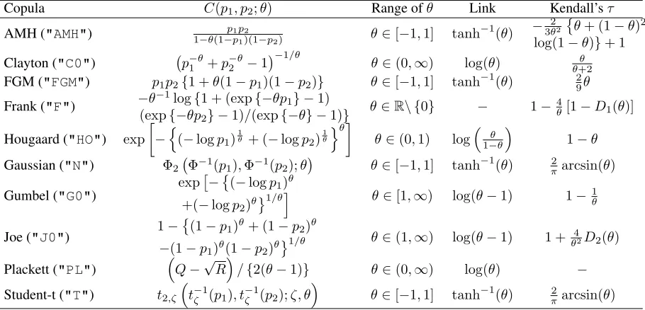
marginal cdfs and a functionCthat binds them together. The copulae (as well as rotated versions

of these) implemented inGJRMare reported in Table 2 which also shows the relation between θ

and the Kendall’sτ coefficient which is a more interpretable measure of association that lies in the

customary range[−1,1].

The marginal distributions of Y₁∗ andY₂∗ are specified through parametric cdfs and densities

denoted as Fm(y∗m|µm, σm, νm) and fm(y∗m|µm, σm, νm), for m = 1,2, where µm, σm and νm represent sometimes location, scale and shape (Rigby & Stasinopoulos, 2005). ForY₁∗ we have

considered the Gaussian, logistic and Gumbel distributions withµ1 = 0andσ1 = 1(which yield

"probit", "logit" and"cloglog"link functions, respectively), whereas forY₂∗ we have

considered the two and three parameter distributions described in Table 2 of Marra & Radice

(2017a). These are the normal ("N"), log-normal ("LN"), Gumbel ("GU"), reverse Gumbel

("rGU"), logistic ("LO"), Weibull ("WEI"), inverse Gaussian ("iG"), gamma ("GA"), Dagum

("DAGUM"), Singh-Maddala ("SM"), beta ("BE"), and Fisk ("FISK") distributions. Note that

the adopted notation reflects the fact that we have considered two and three parameter distributions

for the outcome equation. However, our framework can in principle accommodate distributions

with any number of parameters. Argument margins of gjrm() in GJRM allows the user to

employ the desired link function and outcome distribution and can be set to any of the values

Copula C(p1, p2;θ) Range ofθ Link Kendall’sτ

AMH ("AMH") p1p2

1−θ(1−p1)(1−p2) θ∈[−1,1] tanh

−1

(θ) −

2 3θ2

θ+ (1−θ)2 log(1−θ)}+ 1

Clayton ("C0") p−₁θ+p₂−θ−1−1/θ

θ∈(0,∞) log(θ) _θ+2θ

FGM ("FGM") p1p2{1 +θ(1−p1)(1−p2)} θ∈[−1,1] tanh−1(θ) 2₉θ

Frank ("F") −θ

−1_{log{1 + (exp{−θp} 1} −1) (exp{−θp2} −1)/(exp{−θ} −1)}

θ∈R\ {0} − 1−4θ[1−D1(θ)]

Hougaard ("HO") exp

−n(−logp1)1θ + (−logp2)

1

θ

oθ

θ∈(0,1) log₁₋θ_θ 1−θ

Gaussian ("N") Φ2 Φ−1(p1),Φ−1(p2);θ

θ∈[−1,1] tanh−1(θ) 2

πarcsin(θ)

Gumbel ("G0")

exp

−

(−logp1)θ

+(−logp2)θ

1/θi _θ∈_[1,∞_{) log(θ}−_{1) 1}−1

θ

Joe ("J0") 1−

(1−p1)θ+ (1−p2)θ

−(1−p1)θ(1−p2)θ

1/θ θ∈(1,∞) log(θ−1) 1 +_θ42D2(θ)

Plackett ("PL") Q−√R/{2(θ−1)} θ∈(0,∞) log(θ) −

Student-t ("T") t2,ζ

t−_ζ1(p1), t−_ζ1(p2);ζ, θ θ∈[−1,1] tanh−1(θ) _π2arcsin(θ)

Table 2: Definition of copulae implemented inGJRM, with corresponding parameter range of association parameter

θ, link function ofθ, and relation between Kendall’sτandθ.Φ2(·,·;θ)denotes the cumulative distribution function (cdf) of a standard bivariate normal distribution with correlation coefficientθ, andΦ(·)the cdf of a univariate standard normal distribution.t2,ζ(·,·;ζ, θ)indicates the cdf of a standard bivariate Student-t distribution with correlationθand

fixedζ∈(2,∞)degrees of freedom, andtζ(·)denotes the cdf of a univariate Student-t distribution withζdegrees of

freedom.D1(θ) = 1_θR₀θ_exp(t_t)−1dtis the Debye function andD2(θ) =R₀1tlog(t)(1−t)2(1θ−θ)dt. QuantitiesQand Rare given by1 + (θ−1)(p1+p2)andQ2_{−4θ(θ−1)p1p2, respectively. The Kendall’sτ for"PL"is computed}

4.3

Some estimation details and further considerations

The log-likelihood of the copula sample selection model can be written as

`(δ) =

n X

i=1

(1−y1i) log{F1(0)}+y1ilog [f2(y2i|µ2i, σ2i, ν2i) (1−hi)],

where

hi =

∂C(F1(0), F2(y2i|µ2i, σ2i, ν2i))

∂F2(y2i|µ2i, σ2i, ν2i)

. (4)

The distributional parameters are defined as µ1 = gµ−11(ηµ1i), µ2i = g

−1

µ2(ηµ2i), σ2i = g

−1

σ2(ησ2i),

ν2i =g−ν21(ην2i)andθi = g

−1

θ (ηθi), where theg’s are link functions which ensure that the restric-tions on the parameter spaces are maintained. Parameter vectorδis made up of the distributional

parameters which in turn containβµ1,βµ2,βσ2,βν2andβθ(the coefficient vectors associated with

ηµ1i, ηµ2i, ησ2i, ην2i and ηθi). Parameter estimation is achieved using an extended version of the

efficient and stable trust region algorithm introduced by Marra & Radice (2017a). In particular,

the algorithm uses the analytical score and Hessian of`(δ), which have been derived in a modular fashion. For instance, the score vector is made up of

∂`(δ)

∂βµ1

=

n X

i=1

1−y1i

F1(0)

− y1i

1−hi

∂hi

∂F1(0)

∂F1(0)

∂ηµ1i

Xµ1i,

∂`(δ)

∂βµ2

=

n X

i=1

y1i

f2(y2i|µ2i, σ2i, ν2i)

(1−hi)

∂f2(y2i|µ2i, σ2i, ν2i)

∂µ2i

−

f2(y2i|µ2i, σ2i, ν2i)

∂hi

∂F2(y2i|µ2i, σ2i, ν2i)

∂F2(y2i|µ2i, σ2i, ν2i)

∂µ2i

∂µ2i

∂ηµ2i

Xµ2i,

(5)

∂`(δ)/∂βσ2 and∂`(δ)/∂βν2 (whose expressions are not reported here since they very similar to

(5)), and

∂`(δ)

∂βθ

=

n X

i=1

y1i

hi −1

∂hi

∂θi

∂θi

∂ηθi

Xθi,

whereXµ1i, Xµ2i andXθirepresent the covariate vectors associated with their respective additive

predictors. Looking at equation (5), we see that there are two components which depend on the

structure of the equation will be unaffected by the specific choices made. This means that it will

be easy to extend our algorithm to other copulae and marginal distributions not considered in this

work, as long as their cdfs and probability density functions are known and their derivatives with

respect to their parameters exist. As shown in Marra & Radice (2017a), if the equations of the

joint model contain flexible functions of covariates then a penalty term is employed in estimation,

in which case the approach becomes penalised likelihood-based.

The proposed approach offers a lot of flexibility for modelling MNAR data. For choosing a

suitable copula function, link function and response distribution, as well as selecting covariates

in the model’s additive predictors if required, we recommend using the Akaike information

crite-rion (AIC) and/or Bayesian information critecrite-rion (BIC), normal Q-Q plots of normalized quantile

residuals and hypothesis testing (Marra & Radice, 2017a). Note that as far as the choice of link

function is concerned, as pointed out in Section 4.2, we have considered the Gaussian, logistic

and Gumbel distributions (with location and scale parameters equal to0and1) which yield pro-bit, logit and cloglog links. In this case, since the response is binary, residual analysis would not

be informative unless residuals could be grouped in a meaningful way (e.g., Collett, 2002). We

therefore recommend avoiding looking at residual plots for the selection equation and doing a

sensitivity analysis using the links available.

Reliable point-wise ‘confidence’ intervals for any linear and non-linear function of the model

coefficients are obtained using the posterior distribution δ ∼ N· ( ˆδ,−Hˆ−_p1), where Hp is the model’s Hessian. The rationale for using this result post-estimation is provided in Marra & Wood

(2012) and Marra & Radice (2017a), for instance. These papers show that using the above

poste-rior distribution yields confidence intervals with better frequentist properties than those obtained

using a frequentist approach itself. Other advantages of using the Bayesian result are that the

distribution of non-linear functions of the model parameters can easily be obtained by posterior

simulation and that the resulting distribution need not be symmetric. Note that if the model’s

addi-tive predictors do not include terms which require penalization during model fitting (like smooth

functions of continuous covariates), then the expressions for the frequentist and Bayesian

covari-ance matrices are identical.

Radice, 2017b). For instance,

fl <- list(y1 ~ x1 + x2, y2 ~ x1)

md <- gjrm(fl, Model = "BSS", margins = c("logit", "WEI"), BivD = "PL")

whereflis a list containing the selection and outcome equations, respectively, and"BSS"stands

for bivariate sample selection model.

4.4

Multiple imputation

In this section we introduce a flexible imputation procedure that generates plausible imputed

val-ues from the proposed copula selection model for handling non-Gaussian (continuous) outcomes

that are MNAR. The general idea of MI can be summarised in three steps: 1) generate more than

one complete data set by filling each missing value with draws from the posterior distribution of

the missing data given the observed data; 2) apply the model of interest to each of the imputed

data sets; 3) combine the resulting parameter estimates of interest, for example average treatment

effects and standard errors, obtained from the analyses of the different imputed data sets. The

standard implementation of MI is valid under the MAR assumption. However, MI can also be

used when the missing data mechanism is suspected to be MNAR (Rubin, 1987; Schafer, 1999).

Recent studies have considered the MI approach for handling MNAR in the context of selection

models, for example, assuming bivariate normality under the classical selection model (Galimard

et al., 2016), and bivariate t−distribution (Ogundimu & Collins, 2017). The proposed MI

ap-proach allows us to model more flexibly the selection and outcome models in that several types of

marginal and bivariate distributions can be employed when specifying the joint model.

Given the flexibility afforded by copulae, we considered a joint modelling approach to MI,

although fully conditional specification could also be adopted; the equivalence between the two

approaches are discussed elsewhere (Liu et al., 2014; Hughes et al., 2014). From a Bayesian

perspective, we can consider the missing values as a set of additional (unknown) parameters and

data given the observed data

f(y2|y1 = 0) =

Z ZZ

f(y2|y1 = 0,δ)f(δ|y1, y2)dδ, (6)

wheref(y2|y1 = 0,δ)represents the conditional distribution of the missing values, andf(δ|y1, y2)

is the posterior distribution ofδ. In order to obtain plausible imputed values from (6), we first draw

˜

δ fromf(δ|y1, y2)and then drawy˜fromf(y2|y1 = 0,δ = ˜δ). Little & Rubin (1987) suggested

using the asymptotic distribution of the maximum likelihood estimates since it propagates the

uncertainty in the estimated coefficientsδˆ, and are typically readily available. Here, we employ

δ ∼ N· ( ˆδ,−Hˆ−_p1) which, as mentioned in Section 4.3, can provide more reliable confidence intervals in our context. The conditional density of the missing outcomes can be derived from

joint distribution (3). That is,

f(y2|y1 = 0;δ) =

∂F(y2|y1 = 0;δ)

∂y2

= ∂

∂y2

F(0, y2;δ)

F1(0)

= 1

F1(0)

∂F(0, y2;δ)

∂y2

= 1

F1(0)

∂C(F1(0), F2(y2|µ2, σ2, ν2)

∂F2(y2|µ2, σ2, ν2)

∂F2(y2|µ2, σ2, ν2)

∂y2

= 1

F1(0)

h f2(y2|µ2, σ2, ν2).

(7)

whereh is defined in equation (4). We propose sampling from f(y2|y1 = 0;δ) using an

accep-tance/rejection approach (e.g., Robert & Casella, 2005). This method requires the use of a known

distribution (also called instrumental) that has the same support as that of the target distribution

we need to draw from. In our context, it is sensible to employf2(y∗2|µ2, σ2, ν2)as the instrumental

probability density function (pdf). The algorithm proceeds by drawing a candidatey˜from the in-strumental pdf and then accept it with probability proportional tof(˜y|y1 = 0;δ)/f(˜y|µ2, σ2, ν2).

The constant of proportionality, given by1/M, corresponds to the probability of acceptance and

M must satisfy the inequalityt(˜y) =f(˜y|y1 = 0;δ)/f(˜y|µ2, σ2, ν2)≤M.

M is chosen by maximisingt(˜y)using a trust-region algorithm which typically provides more accurate results than standard alternatives (e.g., Nocedal & Wright, 2006). To prevent the

candidatey˜, using a differentiable and monotone function, such that its range is unbounded. For example, in the case of distributions with a positive support we use transformation yˇ = log(˜y). The use of such algorithm requires computing first and second derivatives. These are given by

dt(˜y)

dyˇ = 1

F1(0)

h0 f2(˜y|µ2, σ2, ν2)

dy˜

dyˇ

and

d2t(˜y)

dyˇ2 =

1

F1(0)

h00(f2(˜y|µ2, σ2, ν2)) 2

+h0∂f2(˜y|µ2, σ2, ν2) ∂y˜

dy˜

dyˇ

2

+dt(˜y) ˜

y d2y˜

dyˇ2,

whereh0 andh00are the first and second derivative ofhwhich are defined as

h0 = ∂

2_C(F

1(0), F2(˜y|µ2, σ2, ν2))

∂F2(˜y|µ2, σ2, ν2)2

and h00 = ∂h

0

∂F2(˜y|µ2, σ2, ν2)

.

Having obtained all the components needed to sample from (7), the algorithm proposed for

impu-tation reduces to two steps: i) drawδ˜fromN( ˆδ,−Hˆ_p−1); ii) draw a candidatey˜fromf(y2|y1 =

0,δ = ˜δ).

The last step in the MI process consists of combining the estimates obtained from the

anal-ysis of all imputed data sets, for example, by applying what is commonly known as Rubin’s

rules (Rubin, 1987). Letδˆ(1), . . . ,δˆ(nc) denote the estimates for the nc completed data sets with corresponding variance/covariance matrices represented byVˆ(1), . . . ,Vˆ(nc). The MI estimate is given byδˆMI =

1

nc Pnc

j=1δˆ

(j) _{(average across the multiple estimates), whereas the corresponding}

variance/covariance matrix is made of two components: the within-imputation varianceWˆMI = 1

nc Pnc

j=1Vˆ

(j) _{and the between-imputation variance Bˆ}

MI =

1

nc−1

Pnc j=1( ˆδ

(j) _−δˆ

MI)( ˆδ(j) −δˆMI)T.

These two components are the combined to giveVˆMI = ˆWMI +

1 + _nc1 BˆMI, where the extra

n−1

c BˆMI term is included to adjust for the finite number of imputations,nc.

When the model contains parametric and smooth components, we can use the Bayesian

pos-terior distributions obtained from the models fitted to the complete data sets to create a global

terior distribution of the parameters and then combine all draws from all models to form a set of

realisations from all posterior distributions.100(1−α)%intervals for the parametric components can be obtained by computing theα/2and1−α/2quantiles of the set. Intervals for the smooth components or non-linear functions of the model parameters are calculated in a similar fashion.

FunctionimputeSS(x, m)inGJRM, wherexis a fittedgjrmobject andmis the number

of sets of imputed values for the outcome of interest, implements the above imputation approach.

5

Monte Carlo simulations

5.1

Data generating process

Through a simulation study, we characterised the relative performance of the copula selection

approach with and without MI compared to widely used sample selection models such as FIML

and 2-step Heckman approach. The data generating process was informed by our motivating

example and previous empirical studies (Sales et al., 2004; Imai, 2009; Alva et al., 2014) in order

to reflect a wide range of MNAR settings typically seen in practice. For example, we considered

scenarios based on different strengths of the MNAR mechanism, alternative proportions of missing

data, and strength of the exclusion restrictions.

The data generating process assumed the following. We generated an exclusion restriction

variableX1 ∼N(0, 1), a prognostic factorX2 ∼N(0.1−0.1X1, 1), and the treatment indicator

P(T = 1|X1) = Φ(0.2+0.3X1). The missingness (Y1) and outcome (Y2) variables were generated

from a joint distribution using copulae as described in Marra & Radice (2017a). The parameters

of the marginals are specified asηµ1 = 1 + 0.4T + 0.3X2+ 0.5X1 andηµ2 = 1 + 0.2T + 0.1X2,

andθ governs the dependence betweenY1 andY2 (this induces MNAR). For the purposes of the

simulations and to make the comparisons with existing methods more straightforward, we have

considered throughout: i) a Gaussian copula (Table 2), ii) a Gamma distributed outcome (where

the mean and skewness were simple functions of the usual shape and scale parameters), iii) a

probit model for the selection, and iv) linear functional forms for bothY2 onX2,X2 onX1andT

onX1.

exclusion restriction). The parameter of interest was the average treatment effect (ATE - obtained

from coefficient of Y2 on T; true value is 0.2) in the outcome model. We varied the following

parameters: % of missing data (by varying the intercept in ηµ2); skewness parameter, 0.5 and

2; strength of MNAR (by varyingθ such thatcor(Y1, Y2) = 0.1,0.25, and0.5); strength of the

exclusion restriction (coefficient ofηµ1 onX1is varied such thatcor(Y1, X1) = 0.1and0.4).

In addition, we have considered three sensitivity analyses which allowed for: i) potential

mis-specification of the ‘true’ outcome distribution (i.e., outcome data were simulated using a

log-normal distribution, but used a gamma for the analysis model); ii) heavier tails for the selection

model by simulating non-response (Y1) from at-distribution instead of normal; and iii) an

alterna-tive data generating process, where the joint model is generated using a marginal and a conditional

distribution instead of copulae (further details are given in Appendix A of the Supplementary

Ma-terial).

For each scenario, we employed 1000 simulated datasets (each dataset included 1000

indi-viduals) and compared the following methods: Full-data (no missing data - ’benchmark’ for the

selection models), full-information maximum likelihood (FIML) assuming bivariate normality,

two-step Heckman selection model, copula selection model with and without MI (we considered

20 imputations throughout although using a larger number did not lead to different conclusions

and only increased the computing time). Performance was assessed according to bias, root mean

squared error (rMSE), and confidence interval (CI) coverage for estimating treatment effects (β1)

in the following outcome model:Y2i =β0+β1Ti+β2X2i+e2i. FIML and the two-step Heckman approach were implemented in thesampleSelection package inR(Toomet & Henningsen,

2008), whereas the copula selection framework used theGJRM Rpackage.

5.2

Results

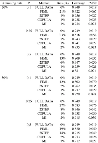
Table 3 reports bias, CI coverage and rMSE across scenarios with slightly skewed data (skewness

factor is 0.5), and alternative strengths (θ) of MNAR. Even in such scenarios with small

devia-tions from normality, ATE estimates using FIML were biased and CI coverage was ’poor’ (below

nom-and ’stronger’ MNAR (θ = 0.25and0.5) treatment effect estimates were slightly biased and less precise (larger rMSE). Copula selection models, estimated by either maximum likelihood or MI

led to unbiased estimates, CI coverage close to nominal levels and the lowest rMSE across all

sce-narios. Figure 2 suggests that the differences in relative performance across alternative approaches

were maintained in scenarios with highly skewed data (skewness factor was 2). In particular, the

2-step Heckman model appeared to be less robust to large departures from the bivariate normal

assumption, and provided larger biases and less precise estimates compared to the copula selection

models.

Methods

b1 -0.2

0.0 0.2 0.4 0.6 0.8 1.0

θ=0.1

20%

θ=0.25 θ=0.5

2STEP COPULA MI

50%

2STEP COPULA MI 2STEP COPULA MI

-0.2 0.0 0.2 0.4 0.6 0.8 1.0

Figure 2: Estimated parameter of interest (AT E[) according to method for scenarios with highly skewed data, increasing levels of θ and alternative % missing data. The boxplots show bias and variation, as median, quartiles and 1.5 times interquartile range for the estimated parameter across the 1000 replications. The dashed lines are the true values. 2STEP: 2-step Heckman model, COPULA: copula selection model using penalized ML; MI: copula selection model using MI.

Table 3: Percent bias, rMSE, and confidence interval coverage for treatment effect (true [

AT E is 0.2) according to method for scenarios with slightly skewed data (skewness factor is 0.5).

% missing data θ Method Bias (%) Coverage rMSE

20% 0.1 FULL DATA 0% 0.949 0.019

FIML 21% 0.422 0.067

2STEP 1% 0.956 0.027

COPULA 1% 0.938 0.023

MI 1% 0.934 0.023

0.25 FULL DATA 0% 0.949 0.019

FIML 23% 0.516 0.054

2STEP 5% 0.943 0.029

COPULA 1% 0.941 0.022

MI 2% 0.935 0.023

0.5 FULL DATA 0% 0.949 0.019

FIML 13% 0.809 0.035

2STEP 6% 0.947 0.030

COPULA 1% 0.939 0.021

MI 2% 0.38 0.021

50% 0.1 FULL DATA 0% 0.949 0.019

FIML 12% 0.802 0.070

2STEP 2% 0.962 0.035

COPULA 1% 0.937 0.029

MI 1% 0.929 0.028

0.25 FULL DATA 0% 0.949 0.019

FIML 27% 0.683 0.076

2STEP 8% 0.946 0.042

COPULA 1% 0.938 0.030

MI 2% 0.915 0.030

0.5 FULL DATA 0% 0.949 0.019

FIML 19% 0.820 0.050

2STEP 14% 0.915 0.049

COPULA 2% 0.933 0.026

MI 3% 0.912 0.027

Figure 3 describes the relative performance of the different selection approaches with a ‘weak’

exclusion restriction, i.e. correlation between Y1 and X1 was 0.1 (as in the REFLUX study).

As anticipated, estimates by the Heckman model are highly imprecise as the 2-step approach

relies more heavily on the presence of a valid exclusion restriction. Both copula-based selection

approaches perform relatively well across all scenarios; for example, rMSE from these methods

is only slightly (around 10%) higher compared to the scenarios with ‘strong’ exclusion restriction

(presented in Figure 2).

Methods b1

-2 0 2

θ=0.1

20%

θ=0.25 θ=0.5

2STEP COPULA MI

50%

2STEP COPULA MI 2STEP COPULA MI

-2 0 2

Figure 3: Estimated parameter of interest (AT E[) according to method for scenarios with ’weak’ exclusion restriction (cor(Y1, X1) = 0.1), increasing levels of θ and alternative % missing data.

The dashed lines are the true values. 2STEP: 2-step Heckman model, COPULA: copula selection model using ML; MI: copula selection model using MI.

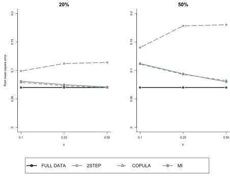
Figure 4 presents the results for settings where the copula model was slightly misspecified

(the copula model assumes gamma when the ’true’ outcome data was log-normal). Both copula

than the 2-step Heckman approach. The plot suggests that the higher the θ (the stronger the

MNAR) the more precise estimates the copula approaches provide. Results for the remaining

sensitivity analyses (alternative DGP andt-distributed non-response) are reported in Appendix B

of the Supplementary Material.

20%

q

Root mean square error

0.1 0.25 0.50

0

0.05

0.1

0.15

0.2

50%

q

0.1 0.25 0.50

0

0.05

0.1

0.15

0.2

FULL DATA 2STEP COPULA MI

Figure 4: Root mean square error according to method for scenarios with misspecification of the copula model, increasing levels of θ and alternative % missing data. FULL DATA: no missing data; 2STEP: 2-step Heckman model, COPULA: copula selection model using ML; MI: copula selection model using MI.

6

Application to REFLUX data

When building the model we investigated the appropriateness of several copulae, link functions

vided the lowest BIC/AIC. Post-estimation normal Q-Q plots suggested that the Gumbel

distribu-tion provided a good fit for the (observed) QALY endpoint (Appendix C, Supplementary Material).

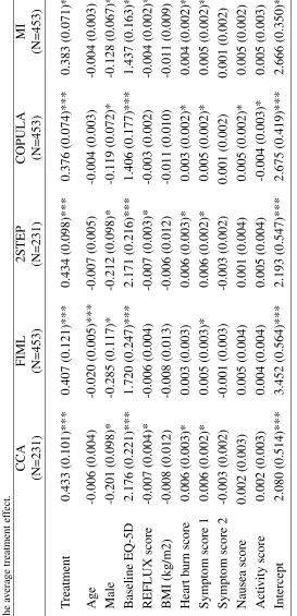
The results from applying the various selection models to the REFLUX data are reported in

Table 4. We followed the same regression adjustment used in the primary analysis of these data

(Grant et al., 2013). The outcome linear model included key prognostic factors, such as age,

gender, baseline HRQL (both REFLUX-specific and generic) and body mass index. The missing

data model for each method included all the covariates used in the analysis model, other patient

characteristics, such as education and employment status, reported in Table 1, and the variables

that met the exclusion restriction (patient’s views about medicine). The parameter of interest was

the treatment effect of surgery on the QALY.

There was strong evidence that patients receiving laparoscopic surgery had better QALY five

years after the intervention than those receiving standard medical care. This effect was somewhat

larger for the complete cases, FIML and Heckman model compared to the copula selection model

and MI. There was some evidence that five-year QALY was associated with baseline quality of life

score, gender, heart burn and symptoms scores, although the strength and statistical significance

of the regression coefficients for these prognostic factors differed across methods. The copula

se-lection models led to substantially smaller standard errors for all regression coefficients, including

treatment effect, compared to the other approaches (as suggested more generally in our

simula-tion study). For example, the MI approach (which provided the most precise estimates) produced

standard errors that were, on average, over 30% lower than those from 2-step Heckman or FIML.

7

Discussion

With missing not at random data, statistical inference fundamentally rests on untestable

assump-tions about the missing data mechanism. Selection models can make plausible assumpassump-tions

regard-ing the missregard-ing data by allowregard-ing for departures from the standard missregard-ing-at-random assumption.

However, the use of selection models for handling MNAR data requires that the analyst recognises

the additional, untestable assumptions imposed by these models. Of particular concern (and the

outcome data such as patient-reported quality of life responses.

This paper discusses a flexible copula-based selection model, which can help make more

plau-sible assumptions about the distribution of the data and offer flexibility about the choice of joint

model for both the outcome and non-response. The modularity of the estimation approach allows

for easy inclusion of potentially any parametric continuous marginal distribution, link function,

and one-parameter copula function as long as the cdf and pdf are known and their derivatives with

respect to their parameters exist. This article also proposes a flexible imputation procedure that

generates plausible imputed values from the copula selection model. The methods can be

read-ily implemented viagjrm()in the RpackageGJRM (Rcode is provided in Appendix C of the

supplementary material).

Through simulations we have studied the performance of the copula selection models across a

wide range of MNAR settings. The proposed approach provided lower bias and root mean square

error compared to popular selection model approaches such as FIML and 2-step Heckman

ap-proach across all scenarios considered. Our method improves thestatus quo particularly in the

absence of valid exclusion restrictions, which tend to be rare in medical and epidemiological

stud-ies. In addition, our simulation results suggested that the copula selection approach is somewhat

robust to (some degree of) misspecification of the outcome and selection equations. Note that

it may be difficult to simulate the potentially highly complex processes that likely underlie the

relation between the missingness mechanism and outcome of interest. Therefore, in practical

ap-plications, it is not possible to determine with certainty how the model assumptions and/or lack

of valid exclusion restrictions may affect the empirical results. Nevertheless, our findings suggest

that the copula approach has merit in dealing with missingness not at random and we believe that

the approach discussed in this paper is a useful addition to the statistical toolbox.

A major strength of the copula framework is that it can be easily embedded in sensitivity

analy-sis to alternative missing data assumptions, as widely recommended by methodological guidelines

for addressing MNAR data (Carpenter & Kenward, 2013; Sterne et al., 2009; Molenberghs et al.,

2014). In fact, the true missing data mechanism (and data distribution) will always be unknown,

and sensitivity analyses provide a helpful framework for assessing how conclusions may differ

outcome and selection (MNAR mechanisms), the copula approach enables the analyst to assess

whether the study’s conclusions are robust to key parametric assumptions such as the functional

form of outcome and selection models, and data distribution. In addition, the fact that the copula

approach can be implemented with MI, makes it particularly attractive for medical and

epidemio-logical researchers given their familiarity with MI for handling missing data.

There are some aspects of the proposed modelling approach that have scope for improvement

and provide direction for future research. Firstly, for comparative purposes we have assumed

linear covariate effects throughout. However, incorporating penalised regression splines in the

discussed copula framework to allow for various degrees of non-linear effects is straightforward

and already implemented in our software (e.g., Marra & Radice, 2017a). Secondly, this study

focused on handling missing outcome data. In many settings, there will be both missing outcomes

and covariates. In such settings, multiple imputation approaches such as that proposed in this

paper can be easily extended to accommodate the missingness both in covariates (typically

assum-ing MAR) and outcomes (MNAR). Extendassum-ing and embeddassum-ing our proposed MI approach within

popular MI software, such as theRpackagemice will further encourage the uptake of the

cop-ula methodology. Thirdly, another area which warrants further consideration is longitudinal data.

Longitudinal settings typically poses further challenges to joint selection models as these often

re-quire additional parametric assumptions, for example about the longitudinal correlation structure.

Finally our proposed approach can be extended to settings where decision problem requires joint

inferences for more than one outcome (Filippou et al., 2017) or addressing hierarchical and/or

spatial effects (Marra et al., 2017).

References

Alva, M., Gray, A., & et al (2014). The effect of diabetes complications on health-related quality

of life: the importance of longitudinal data to address patient heterogeneity.Health Econ, 23(4),

487–500.

Prac-Chen, S. & Zhou, Y. (2010). Semiparametric and nonparametric estimation of sample selection

models under symmetry. Journal of Econometrics, 157, 143–150.

Chib, S., Greenberg, E., & Jeliazkov, I. (2009). Estimation of semiparametric models in the

pres-ence of endogeneity and sample selection. Journal of Computational and Graphical Statistic,

18, 321–348.

Collett, D. (2002). Modelling Binary Data. London: Chapman & Hall/CRC Texts in Statistical

Science.

Daniels, M. & Hogan, J. (2008). Missing Data in Longitudinal Studies: Strategies for Bayesian

Modeling and Sensitivity Analysis. Boca Raton, FL: Chapman and Hall CRC.

Das, M., Newey, W., & Vella, F. (2003). Nonparametric estimation of sample selection models.

Review of Economic Studies, 70, 33–58.

Del Bianco, P. & Borgoni, R. (2006). Handling dropout and clustering in longitudinal multicentre

clinical trials. Statistical Modelling, 6(2), 141–157.

Diggle, P. & Kenward, M. G. (1994). Informative drop-out in longitudinal data-analysis. Journal

of the Royal Statistical Society Series C-Applied Statistics, 43(1), 49–93.

Ding, P. (2014). Bayesian robust inference of sample selection using selection-models.Journal of

Multivariate Analysis, 124, 451–464.

EuroQol (1990). Euroqol-a new facility for the measurement of health-related quality of life.

Health Policy, 16(3), 199–208.

Filippou, P., Radice, R., & Marra, G. (2017). Penalized likelihood estimation of a trivariate

addi-tive probit model. Biostatistics, 18, 569–585.

Galimard, J.-E., Chevret, S., Protopopescu, C., & Resche-Rigon, M. (2016). A multiple imputation

approach for MNAR mechanisms compatible with Heckman’s model. Statistics in Medicine,

Gomes, M., Kenward, M., Grieve, R., & Carpenter, J. (2017). Estimating treatment effects

un-der untestable assumptions with non-ignorable missing data. Statistical Methods in Medical

Research, (under review).

Grant, A. M., Boachie, C., Cotton, S. C., Faria, R., & et al (2013). Clinical and economic

evalua-tion of laparoscopic surgery compared with medical management for gastro-oesophageal reflux

disease: 5-year follow-up of multicentre randomised trial (the reflux trial). Health Technol

Assess, 17(22), 1–167.

Heckman, J. (1974). Shadow prices, market wages and labor supply.Econometrica, 42, 679–694.

Heckman, J. (1979). Sample selection bias as a specification error. Econometrica, 47, 153–162.

Hughes, R. A., White, I. R., Seaman, S. R., Carpenter, J. R., Tilling, K., & Sterne, J. A. C. (2014).

Joint modelling rationale for chained equations. Bmc Medical Research Methodology, 14.

Imai, K. (2009). Statistical analysis of randomized experiments with non-ignorable missing binary

outcomes: an application to a voting experiment. Journal of the Royal Statistical Society Series

C, 58, 83–104.

Lee, D. S. (2008). Training, wages, and sample selection: Estimating sharp bounds on treatment

effects. Review of Economic Studies, 76(11721), 1071–1102.

Little, R. J. & Rubin, D. B. (1987).Statistical Analysis with Missing Data. New York: John Wiley

& Sons.

Liu, J. C., Gelman, A., Hill, J., Su, Y. S., & Kropko, J. (2014). On the stationary distribution of

iterative imputations. Biometrika, 101(1), 155–173.

Marchenko, Y. V. & Genton, M. G. (2012). A heckman selection-t model.Journal of the American

Statistical Association, 107(497), 304–317.

Marra, G. & Radice, R. (2017a). Bivariate copula additive models for location, scale and shape.

Marra, G. & Radice, R. (2017b). GJRM: Generalised Joint Regression Modelling. R package

version 0.1-4.

Marra, G., Radice, R., Bärnighausen, T., Wood, S. N., & McGovern, M. E. (2017). A simultaneous

equation approach to estimating hiv prevalence with non-ignorable missing responses. Journal

of the American Statistical Association, 112(518), 484–496.

Marra, G. & Wood, S. (2012). Coverage properties of confidence intervals for generalized additive

model components. Scandinavian Journal of Statistics, 39, 53–74.

Mason, A., Gomes, M., Grieve, R., Ulug, P., Powell, J., & Carpenter, J. (2017). Development of

a practical approach to expert elicitation for randomised controlled trials with missing health

outcomes: Application to the improve trial. Clinical Trials, (in press).

Molenberghs, G., Fitzmaurice, G. M., Kenward, M., Tsiatis, A. A., & Verbeke, G. (2014).

Hand-book of missing data methodology. Boca Raton, US: Chapman and Hall/CRC.

Newey, W. K. (2009). Two-step series estimation of sample selection models. Econometrics

Journal, 12, S217–S229.

NICE (2013). Guide to the methods of technology appraisal. National Institute for Health and

Care Excelence, London, UK.

Nocedal, J. & Wright, S. J. (2006). Numerical Optimization. New York: Springer-Verlag.

Ogundimu, E. & Collins, G. (2017). A robust imputation method for missing responses and

covariates in sample selection models. Statistical Methods in Medical Research, 26, 1–15.

Pigini, C. (2015). Bivariate non-normality in the sample selection model. Journal of Econometric

Methods, 4, 123–144.

Puhani, P. A. (2000). The heckman correction for sample selection and its critique. Journal of

Economic Surveys, 14, 53–68.

Rigby, R. A. & Stasinopoulos, D. M. (2005). Generalized additive models for location, scale and

Robert, C. & Casella, G. (2005). Monte Carlo Statistical Methods. Springer Texts in Statistics.

Springer New York.

Rubin, D. B. (1987). Multiple Imputation for Nonresponse in Surveys. Wiley Classics Library.

Wiley.

Sales, A. E., Plomondon, M. E., Magid, D. J., Spertus, J. A., & Rumsfeld, J. S. (2004).

Assess-ing response bias from missAssess-ing quality of life data: the heckman method. Health Qual Life

Outcomes, 2, 49.

Schafer, J. (1999). Multiple imputation: a primer. Statistical Methods in Medical Research, 8(1),

3–15.

Sklar, A. (1973). Random variables, joint distributions, and copulas. Kybernetica, 9, 449–460.

Sterne, J. A. C., White, I. R., Carlin, J. B., Spratt, M., Royston, P., Kenward, M. G., Wood, A. M.,

& Carpenter, J. R. (2009). Multiple imputation for missing data in epidemiological and clinical

research: potential and pitfalls. BMJ, 339(b2393), (29 June 2009).

Toomet, O. & Henningsen, A. (2008). Sample selection models in r: Package sampleselection.

Journal of Statistical Software, 27(7), 1–23.

Zhelonkin, M., Genton, M. G., & Ronchetti, E. (2015). Robust inference in sample selection